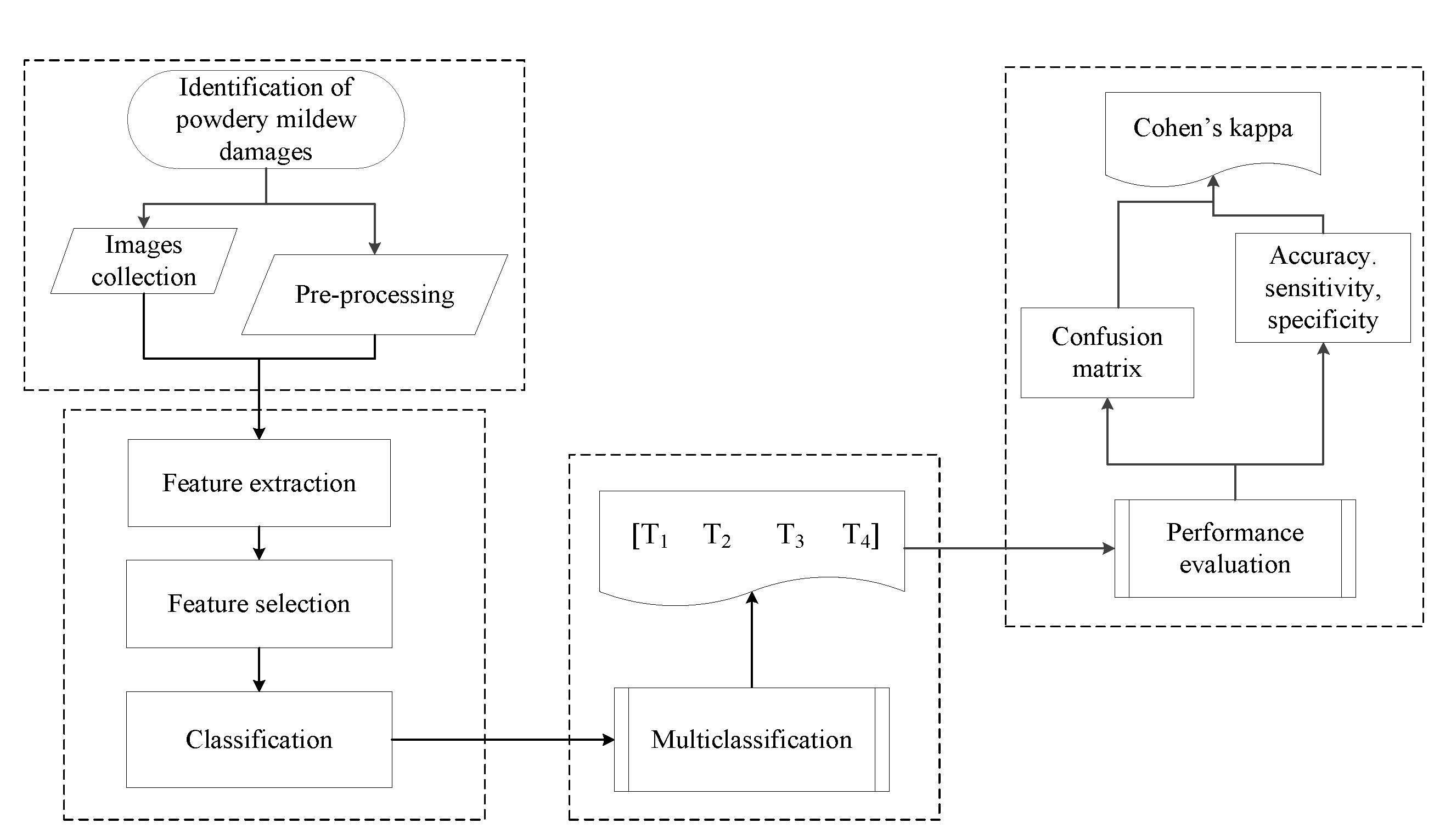
Figure 1.
Proposed methodology for PM damage level detection, where image collection is used for feature extraction and selection. A multiclassification is operated with the results of the classification process. In the end, a performance evaluation is conducted to verify the optimal classification.
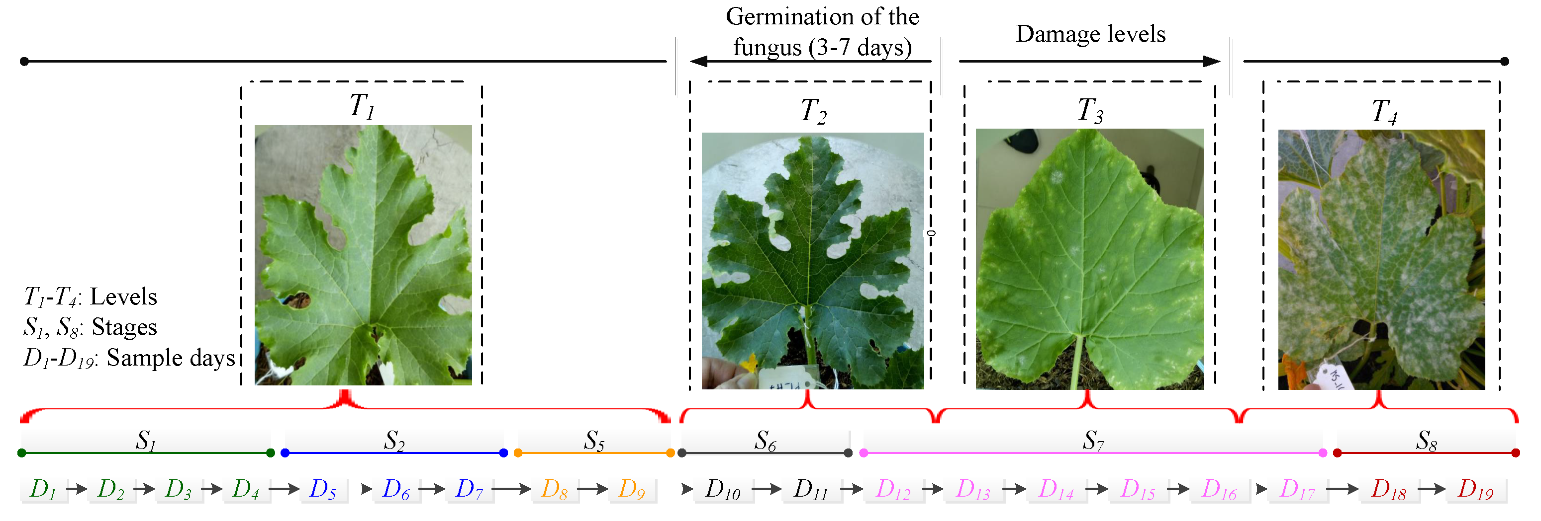
Figure 2.
A timeline of the sampling days and the phenological growth stages to identify PM damage levels. The phenological stages ( to ) and the sampling days ( to ) are considered as basic information. Then, four PM damage levels are defined: for healthy leaves, for leaves with spore in germination, for leaves with the first symptoms, and for diseased leaves.
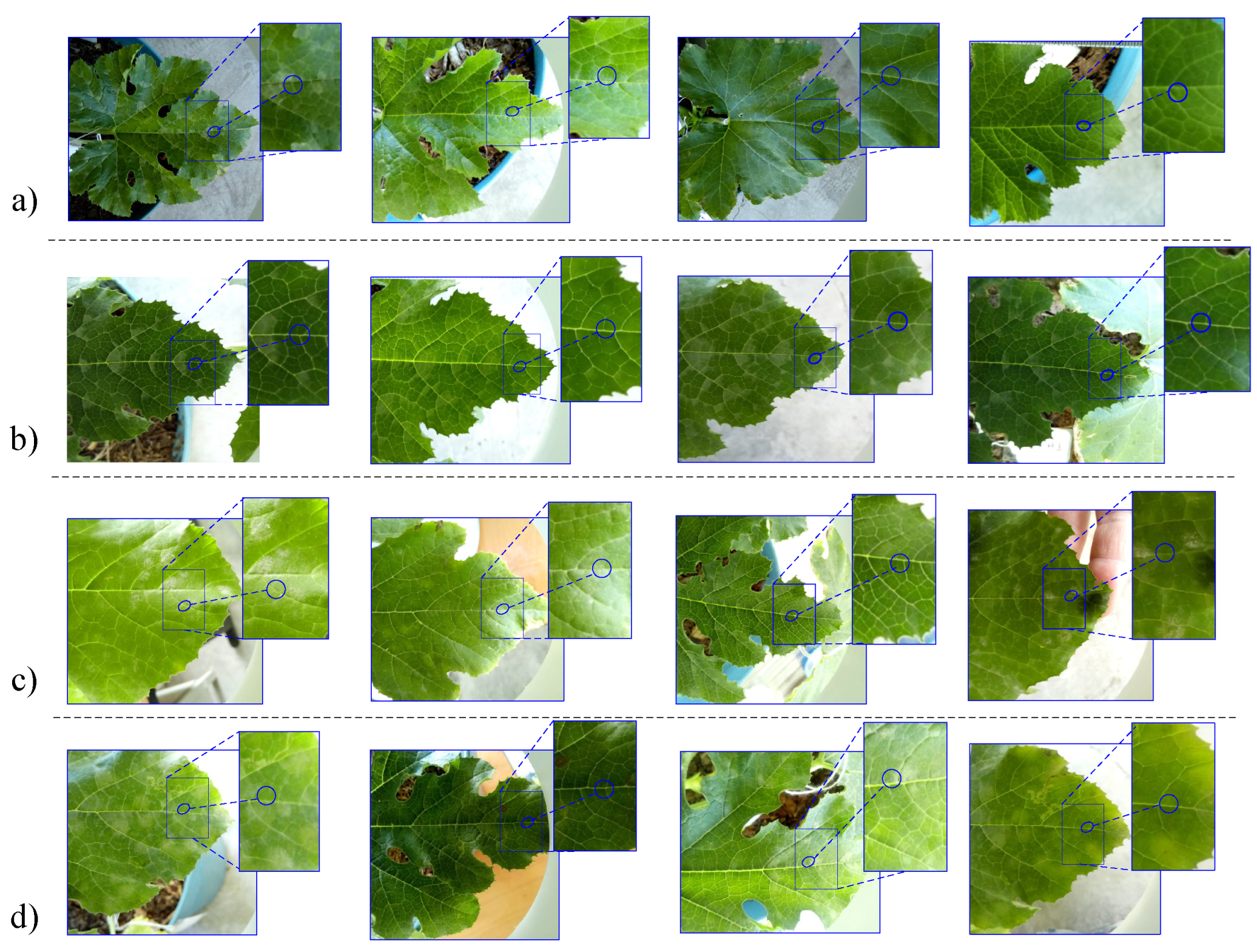
Figure 3.
Visual evaluation of cucurbit leaves where four PM damage levels were defined: (a) : healthy leaves, (b) : leaves with spore in germination, (c) : leaves with the first symptoms, and (d) : diseased leaves.
Figure 3.
Visual evaluation of cucurbit leaves where four PM damage levels were defined: (a) : healthy leaves, (b) : leaves with spore in germination, (c) : leaves with the first symptoms, and (d) : diseased leaves.
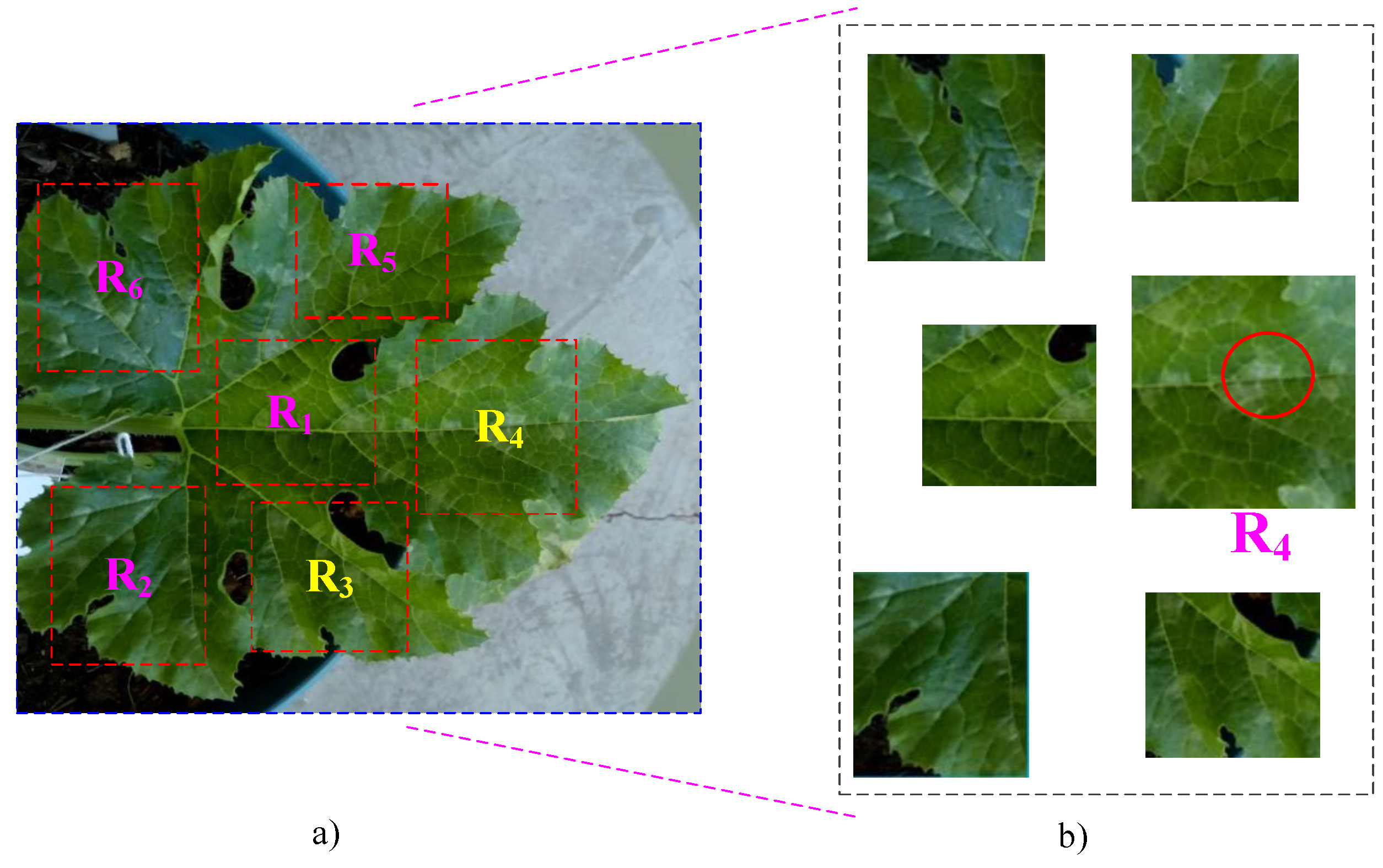
Figure 4.
Exploration by parts of the leaf for the selection of the region of interest (ROI): (a) division of the leaf, central part (), lower right lobe (), upper right lobe (), upper central lobe (), upper left lobe () and lower left lobe (), (b) first symptoms at .
Figure 4.
Exploration by parts of the leaf for the selection of the region of interest (ROI): (a) division of the leaf, central part (), lower right lobe (), upper right lobe (), upper central lobe (), upper left lobe () and lower left lobe (), (b) first symptoms at .
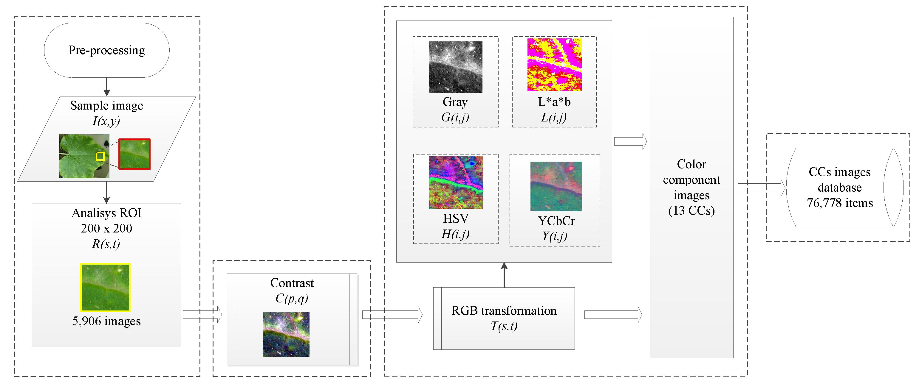
Figure 5.
Preprocessing of the ROI images starting with the color transformation and separation of color components (CCs), where the sample image () is the original image, which is followed by the analysis of ROI results in a new sample in RGB (), then a contrast adjust () is performed to obtain the transformation of the image () in the different color spaces (, , , ) and the separation for color components.
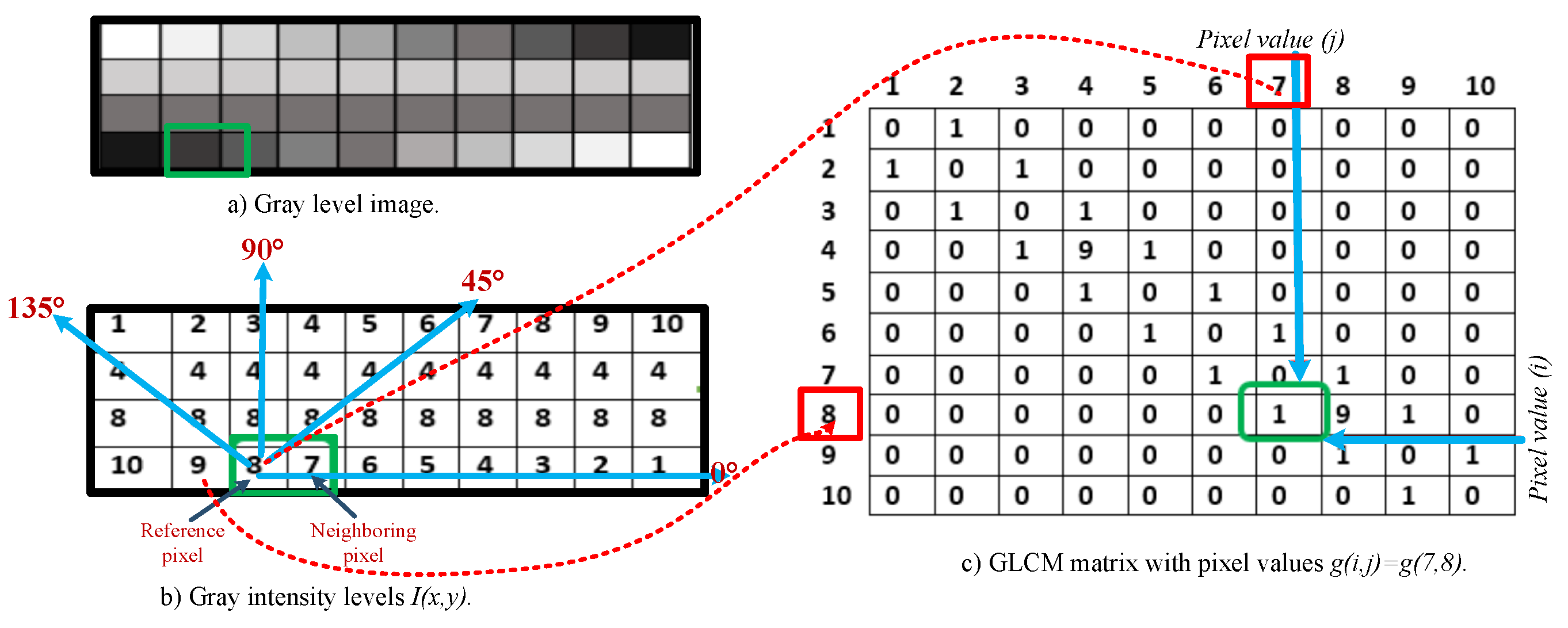
Figure 6.
Calculation of the GLCM matrix in a gray image. The distance is , and the angle is : (a) gray image, (b) gray levels , and (c) GLCM matrix with the paired pixels .
Figure 6.
Calculation of the GLCM matrix in a gray image. The distance is , and the angle is : (a) gray image, (b) gray levels , and (c) GLCM matrix with the paired pixels .
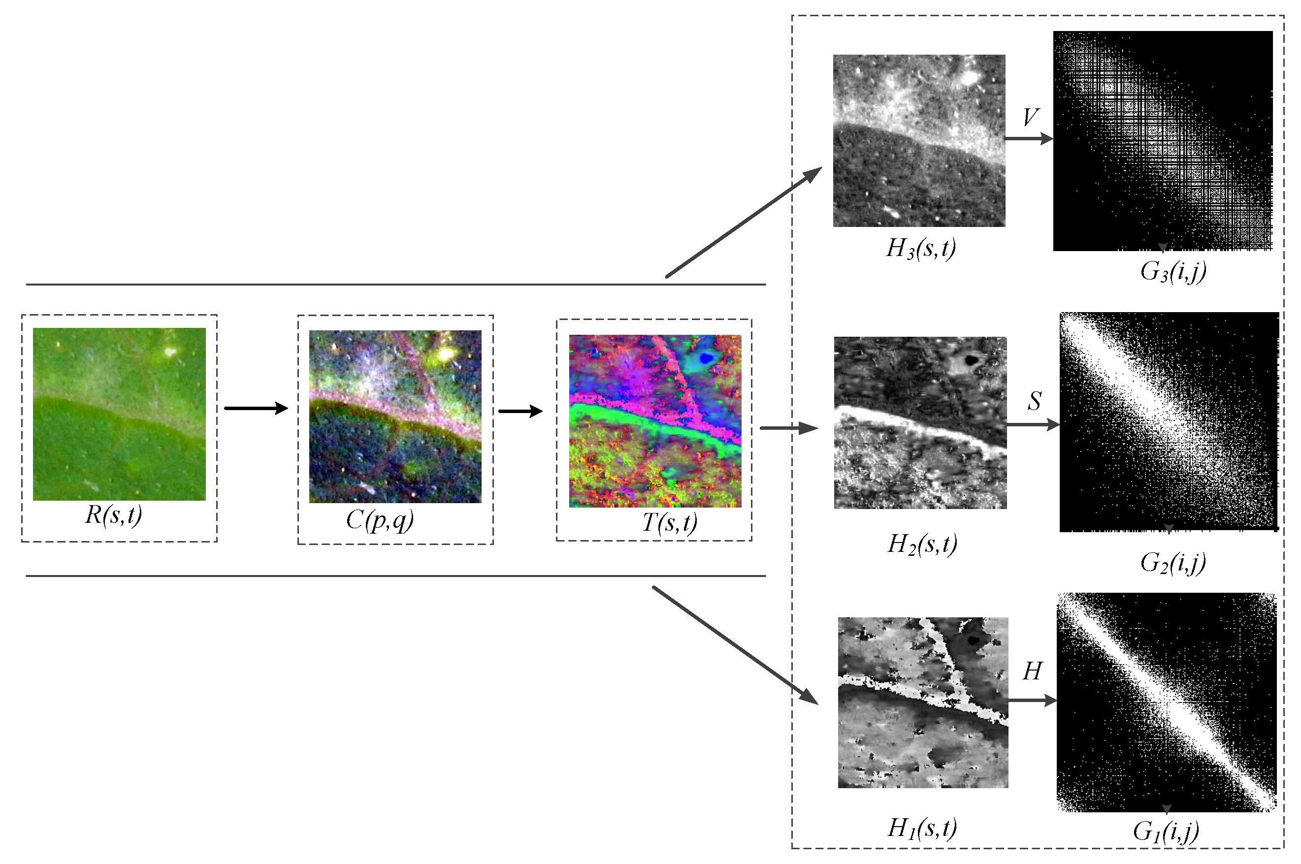
Figure 7.
Processed image ( and ); color transformation (); components , , and ; and their GLCM matrices , , and with 255 gray levels.
Figure 7.
Processed image ( and ); color transformation (); components , , and ; and their GLCM matrices , , and with 255 gray levels.
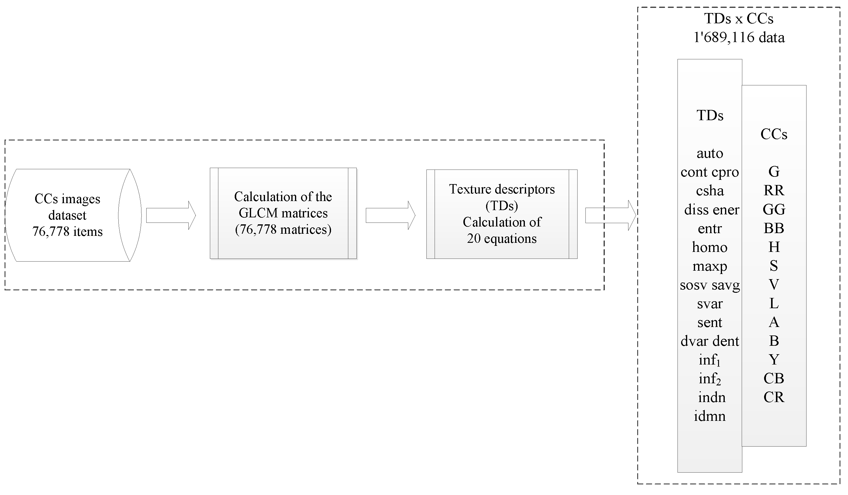
Figure 8.
Process of feature extraction through the color component images.
Figure 8.
Process of feature extraction through the color component images.
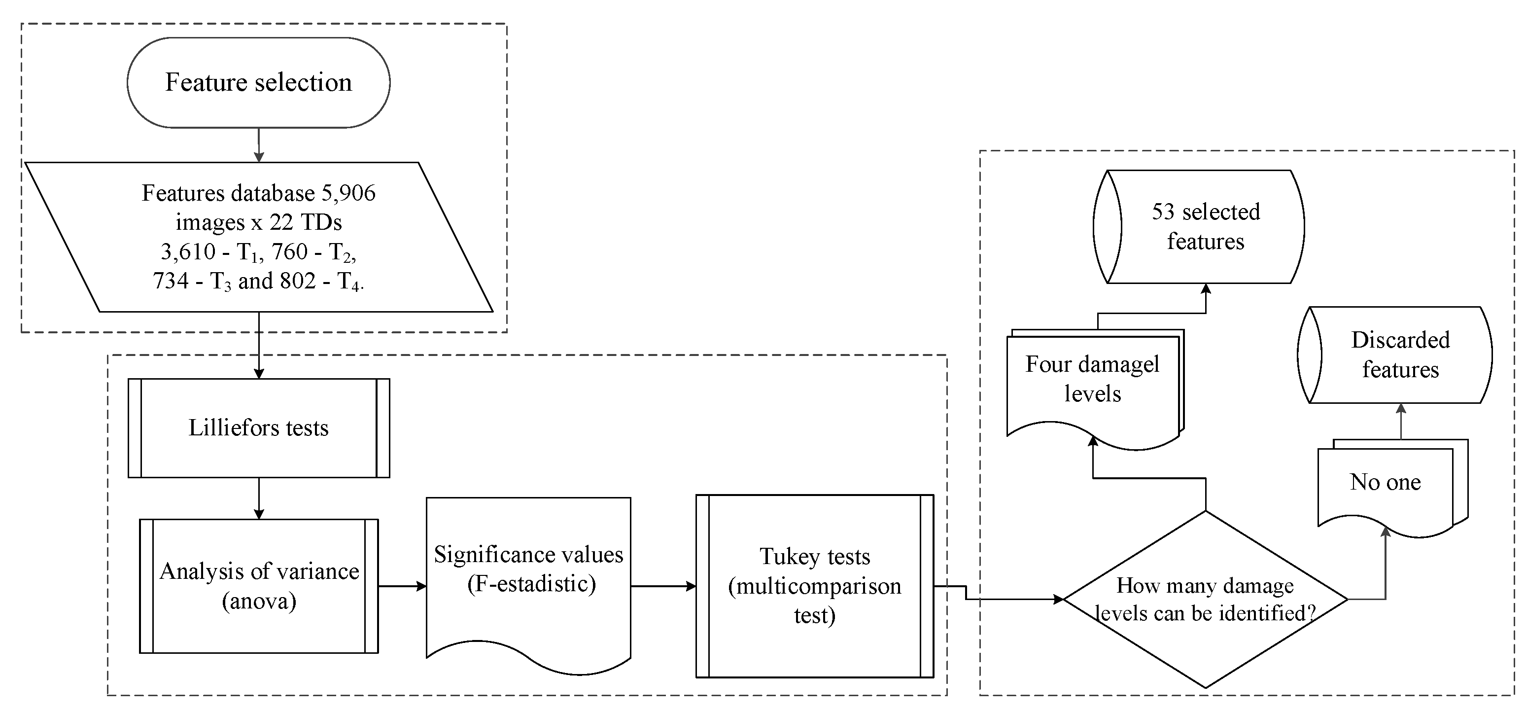
Figure 9.
Feature selection process consists of a Lilliefors test, then an analysis of variance, and Tukey’s test.
Figure 9.
Feature selection process consists of a Lilliefors test, then an analysis of variance, and Tukey’s test.
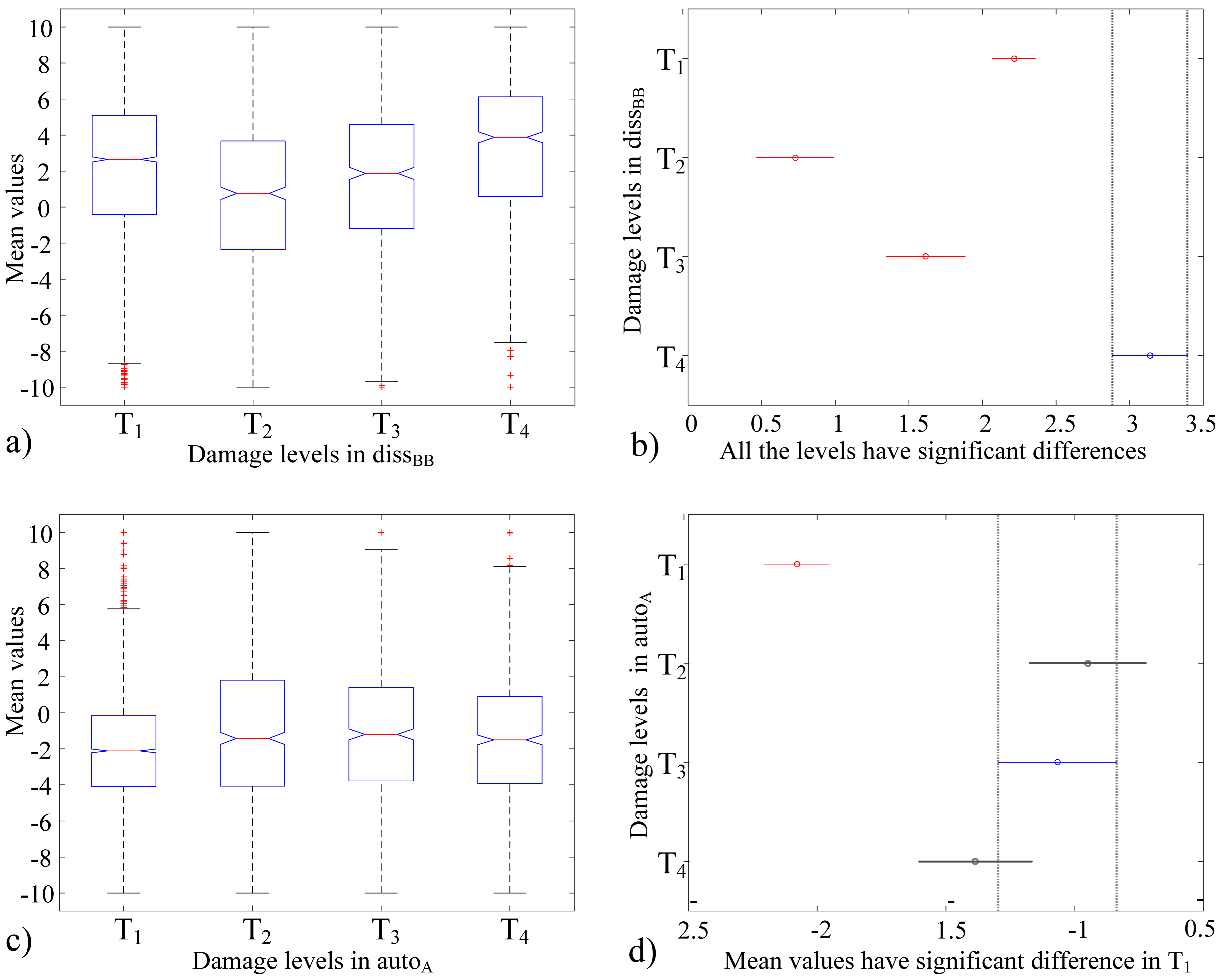
Figure 10.
Results of the ANOVA and Tuke’s test: (a) mean values of the damage levels of diss-BB; (b) Tukey’s test, where the means of the damage levels are significantly different; (c) mean values of the damage levels of auto-A; (d) Tukey’s test, where the means of , , and are equal but significantly different from .
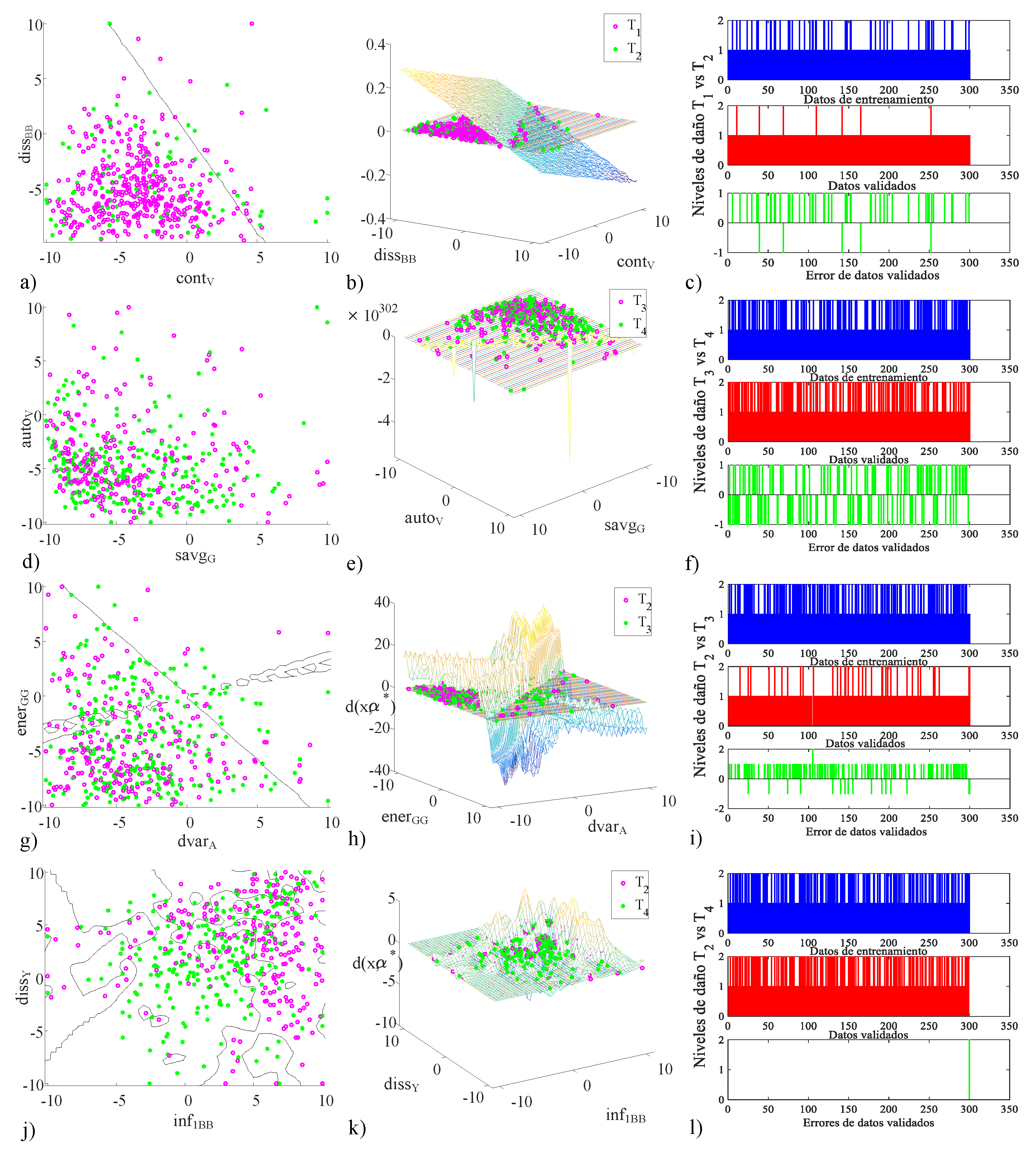
Figure 11.
Kernel selection in the multiclassification system with the feature vectors in different color spaces with the optimal hyperplane: (a) linear kernel in 2D with diss versus cont, (b) 3D optimal hyperplane, (c) training and validation data with error in SVM versus , (d) polynomial kernel in 2D with auto versus savg, (e) 3D optimal hyperplane, (f) training and validation data with error in SVM versus , (g) sigmoidal kernel in 2D with ener versus dvar, (h) 3D optimal hyperplane, (i) training and validation data with the error in SVM versus , (j) radial base function kernel in 2D with diss versus inf con kernel RBF, (k) 3D optimal hyperplane, and (l) training and validation data with the error in SVM versus .
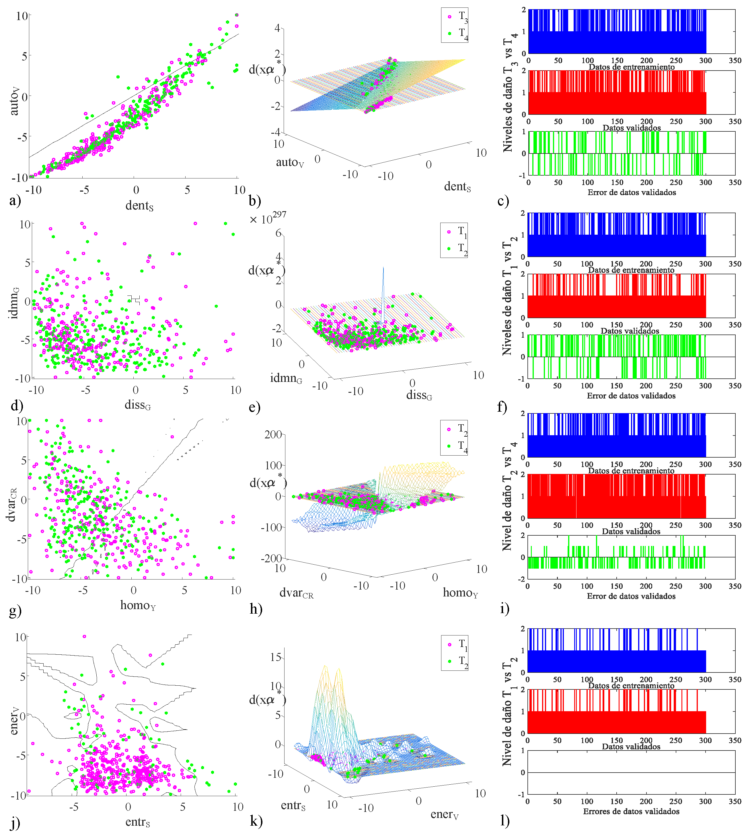
Figure 12.
Kernel selection in the multiclassification system with the feature vectors in different color space with the optimal hyperplane: (a) radial base function kernel in 2D with auto versus dent, (b) 3D optimal hyperplane, (c) training and validating data with the error in the SVM versus , (d) linear kernel in 2D with idmn versus diss, (e) 3D optimal hyperplane, (f) training and validate data with the error in the SVM versus , (g) polynomial kernel in 2D with dvar versus homo, (h) 3D optimal hyperplane, (i) training and validate data with the error in the SVM versus , (j) radial base function kernel in 2D with ener versus entr con kernel RBF, (k) 3D optimal hyperplane, and, (l) training and validate data with the error in the SVM versus .
Figure 13.
One-versus-one multiclassification method. The main inputs are the support vectors ), the validation data for each binary classifier , and . Each block contains the different support vector machines for multiple classification.
Figure 13.
One-versus-one multiclassification method. The main inputs are the support vectors ), the validation data for each binary classifier , and . Each block contains the different support vector machines for multiple classification.
Figure 14.
SVM binary classifiers: (a) test data and SVM-classified data, (b) test data and SVM-classified data, (c) test data and SVM-classified data, (d) test data and SVM-classified data, and (e) test data and SVM-classified data.
Figure 14.
SVM binary classifiers: (a) test data and SVM-classified data, (b) test data and SVM-classified data, (c) test data and SVM-classified data, (d) test data and SVM-classified data, and (e) test data and SVM-classified data.
Figure 15.
SVM binary classifiers with components of the same color space: (a) test data and SVM-classified data, (b) test data and SVM-classified data, (c) test data and SVM-classified data, (d) test data and SVM-classified data, and (e) test data and SVM-classified data.
Figure 15.
SVM binary classifiers with components of the same color space: (a) test data and SVM-classified data, (b) test data and SVM-classified data, (c) test data and SVM-classified data, (d) test data and SVM-classified data, and (e) test data and SVM-classified data.
Table 1.
Texture descriptors (DTs) equations [
4,
17,
18,
19].
Table 1.
Texture descriptors (DTs) equations [
4,
17,
18,
19].
| Equation | DTs | Texture Descriptors |
|---|
| auto | Autocorrelation |
| cont | Contrast |
| corr | Correlation 1 |
| cpro | Cluster Prominence 1 |
| csha | Cluster Shade 1 |
| diss | Dissimilarity |
| ener | Energy |
| entr | Entropy |
| homo | Homogeneity |
| maxp | Maximum Probability 1 |
| sosv | Sum of Squares |
| savg | Sum Average |
| svar | Sum Variance |
| sent | Sum Entropy |
| dvar | Difference Variance 1 |
| dent | Difference Entropy |
| inf | Information Measure of Correlation 2 3 |
| inf | Information Measure of Correlation 2 3 |
| indn | Inverse Difference Normalized |
| idmn | Inverse Difference Moment Normalized |
Table 2.
An example of the results of two features submitted to the Lilliefors test. For each CC (G—gray, R—red, GG—green, BB—blue, H—hue, S—saturation, V—value, L—luminance, A—a * red and green coordinates, B—b * yellow coordinates with blue, Y—luma, CB—Cb chrominance difference of blue, CR—Cr chrominance difference of red). The features are shown with their four damage levels. If the in “ 0 ” appears at any level, the feature is discarded for not complying with the normality condition.
| | Gray | RGB | HSV | L * a * b | YCbCr |
|---|
| | TDs | G | R | GG | BB | H | S | V | L | A | B | Y | CB | CR |
| diss | 1 | 1 | 1 | 1 | 1 | 1 | 1 | 1 | 1 | 1 | 1 | 1 | 1 |
| | 1 | 1 | 1 | 1 | 1 | 1 | 1 | 1 | 1 | 1 | 1 | 1 | 0 |
| | 1 | 1 | 1 | 0 | 1 | 1 | 1 | 1 | 1 | 1 | 1 | 1 | 0 |
| | 0 | 1 | 0 | 0 | 1 | 1 | 0 | 1 | 1 | 1 | 0 | 1 | 1 |
| homo | 1 | 1 | 1 | 1 | 1 | 1 | 1 | 1 | 1 | 1 | 1 | 1 | 1 |
| | 1 | 1 | 1 | 1 | 1 | 1 | 1 | 1 | 1 | 1 | 1 | 1 | 1 |
| | 1 | 1 | 1 | 1 | 1 | 1 | 1 | 1 | 1 | 1 | 1 | 1 | 1 |
| | 1 | 1 | 1 | 1 | 1 | 1 | 1 | 1 | 1 | 1 | 1 | 1 | 1 |
| idmn | 1 | 1 | 1 | 1 | 1 | 1 | 1 | 1 | 1 | 1 | 1 | 1 | 1 |
| | 1 | 1 | 1 | 1 | 1 | 1 | 1 | 1 | 1 | 1 | 1 | 1 | 1 |
| | 1 | 1 | 1 | 1 | 1 | 1 | 1 | 1 | 1 | 1 | 1 | 1 | 1 |
| | 1 | 1 | 0 | 1 | 1 | 1 | 1 | 1 | 1 | 1 | 1 | 1 | 1 |
Table 3.
Examples of results of Tukey’s test by feature listed in order according to the ability to separate the four damage levels of PM.
Table 3.
Examples of results of Tukey’s test by feature listed in order according to the ability to separate the four damage levels of PM.
| Feature | F Statistic | | | | |
|---|
| ener | 184.7 | a | b | c | d |
| corr | 174.7 | a | b | c | d |
| homo | 171.2 | a | b | c | d |
| corr | 158.6 | a | b | c | d |
| ener | 143.2 | a | b | c | d |
| ener | 142.6 | a | b | c | d |
| dent | 134.5 | a | b | c | d |
| sosv | 71.4 | a | b | c | d |
| dvar | 125.5 | a | b | c | d |
| idmn | 124.4 | a | b | c | d |
| cpro | 122.4 | a | b | c | d |
| homo | 119.4 | a | b | c | d |
| entr | 112.7 | a | b | c | d |
| homo | 111.3 | a | b | c | d |
| cont | 109.7 | a | b | c | d |
| dvar | 109.7 | a | b | c | d |
| dvar | 105.9 | a | b | c | d |
Table 4.
Formation of the features vectors with the combination of six TDs features belonging to different color spaces (, …, ), and the features belonging to components of the same color space (, …, ).
Table 4.
Formation of the features vectors with the combination of six TDs features belonging to different color spaces (, …, ), and the features belonging to components of the same color space (, …, ).
| TDs | Vector | Features |
|---|
| Different | | auto, dent, svar, svag, sosv, savg |
| color | | entr, homo, idmn, idmn, dvar, cont |
| space | | dvar, cont, idmn, idmn, idmn, cont |
| combinations | | cont, homo, entr, homo, cpro, idmn |
| | | cont, dvar, dent, ener, ener, corr |
| Same | | sent, entr, idmn, cont, diss, inf |
| color | | dent, entr, auto, svar, sosv, ener |
| space | | diss, savg, idmn, cont, dvar, ener |
| combinations | | diss, homo, corr, idmn, dvar, cont |
| | | diss, savg, idmn, cont, dvar, homo |
Table 5.
Support vector machines with different space color components with the kernels’ linear, polynomial, sigmoidal, and radial base function for the selection of the SVM.
Table 5.
Support vector machines with different space color components with the kernels’ linear, polynomial, sigmoidal, and radial base function for the selection of the SVM.
| Kernel | SVM | p// | R | h | | | % Error |
|---|
| Lineal | | - | 433.36 | 1.0 × 10¹⁵ | 0.0 + 90.74 | 2.4 × 10¹² | 17.4 |
| Lineal | | - | 448.28 | 1.1 × 10¹⁵ | 0.0 + 9.53i | 2.6 × 10¹² | 18.6 |
| Polynomial | | 4 | 3917 | 1.2 × 10¹⁶ | 0.0 + 3.0i | 3105.6 | 30 |
| Polynomial | | 4 | 3989 | 7.1 × 10¹⁶ | 0.0 + 8.7i | 1801.79 | 20.2 |
| Sigmoidal | | 1 | 2192.8 | 1096.5 | 0.0 + 1.67i | 500 | 17.6 |
| Sigmoidal | | 7 | 1614.5 | 8072.3 | 0.0 + 9.1i | 500 | 43.4 |
| RBF | | 0.5 | 0.9978 | 460.17 | 4.1048 | 461.18 | 0 |
| RBF | | 0.5 | 0.9977 | 464.95 | 4.1237 | 465.98 | 0 |
| RBF | | 0.5 | 0.9979 | 493.85 | 4.2359 | 494.87 | 0 |
| RBF | | 0.5 | 0.9979 | 487.92 | 4.2132 | 488.94 | 0 |
| RBF | | 1 | 0.9972 | 413.45 | 3.9135 | 414.60 | 0 |
| RBF | | 1 | 0.9974 | 456.07 | 4.0885 | 457.22 | 0 |
Table 6.
Support vector machines with components of a space color with the kernels’ linear, polynomial, sigmoidal and radial base function for the selection of the SVM.
Table 6.
Support vector machines with components of a space color with the kernels’ linear, polynomial, sigmoidal and radial base function for the selection of the SVM.
| Kernel | SVM | p// | R | h | | | % Error |
|---|
| Lineal | | - | 478.89 | 1.1 × 10¹⁵ | 0.0 + 9.74i | 2.4 × 10¹² | 16.8 |
| Lineal | | - | 455.57 | 1.0 × 10¹⁵ | 0.0 + 8.59i | 2.2 × 10¹² | 15 |
| Polinomial | | 6 | 9.95 × 10¹⁸ | 4.97 × 10²¹ | 0.0 + 26i | 500 | 16 |
| Polinomial | | 6 | 9.28 × 10¹⁸ | 1.24 × 10¹⁵ | 0.0 + 98.2i | 0.0001 | 0 |
| Sigmoidal | | 3 | 2137.45 | 1065.1 | 0.0 + 11.8i | 500 | 17.2 |
| Sigmoidal | | 3 | 2104.09 | 1052.5 | 0.0 + 11.1i | 500 | 17.8 |
| RBF | | 1 | 0.9957 | 458.48 | 4.098 | 460.42 | 0 |
| RBF | | 0.5 | 0.9979 | 469.96 | 4.1434 | 470.95 | 0 |
| RBF | | 0.5 | 0.9978 | 491.79 | 4.2280 | 492.79 | 0 |
| RBF | | 0.5 | 0.9979 | 488.64 | 4.2160 | 489.64 | 0 |
| RBF | | 2 | 0.9799 | 34,676.99 | 25.8 | 35,385.5 | 0 |
| RBF | | 1 | 0.9962 | 764.31 | 5.1414 | 767.17 | 0 |
Table 7.
Computed parameters for the performance evaluation of the classified data , , , , and .
Table 7.
Computed parameters for the performance evaluation of the classified data , , , , and .
| Vector | (%)
| | | | | |
|---|
| 93.1 | 0.832 | 0.965 | 0.887 | 0.035 | 85.8 |
| 88.4 | 0.700 | 0.945 | 0.811 | 0.055 | 75.1 |
| 88.9 | 0.682 | 0.958 | 0.844 | 0.042 | 75.5 |
| 90.0 | 0.728 | 0.957 | 0.850 | 0.043 | 78.4 |
| 91.2 | 0.754 | 0.964 | 0.875 | 0.036 | 81.0 |
Table 8.
Computed parameters for the performance evaluation of the classified data , , , and .
Table 8.
Computed parameters for the performance evaluation of the classified data , , , and .
| Vector | | | | | | |
|---|
| 87.3 | 0.625 | 0.956 | 0.824 | 0.044 | 0.711 |
| 90.8 | 0.776 | 0.952 | 0.843 | 0.048 | 0.808 |
| 94.4 | 0.877 | 0.967 | 0.898 | 0.033 | 0.887 |
| 91.4 | 0.752 | 0.968 | 0.887 | 0.032 | 0.814 |
| 87.3 | 0.678 | 0.938 | 0.786 | 0.062 | 0.728 |
Table 9.
Confusion matrix of the classified test data –.
Table 9.
Confusion matrix of the classified test data –.
| b) SVM- | | | | | Classified | % Correct |
| 71 | 6 | 0 | 2 | 79 | 89.87 |
| 2 | 9 | 0 | 0 | 11 | 81.82 |
| 0 | 0 | 12 | 0 | 12 | 100.00 |
| 2 | 0 | 0 | 2 | 4 | 50.00 |
| Test data | 75 | 15 | 12 | 4 | 106 | |
| % Correct | 94.67 | 60.00 | 100.00 | 50.00 | | 88.68 |
| d) SVM- | | | | | Classified | % Correct |
| 46 | 5 | 2 | 2 | 55 | 83.64 |
| 4 | 7 | 0 | 0 | 11 | 63.64 |
| 3 | 0 | 7 | 0 | 10 | 70.00 |
| 2 | 0 | 0 | 17 | 19 | 89.47 |
| Test data | 55 | 12 | 9 | 19 | 95 | |
| % Correct | 83.64 | 58.33 | 77.78 | 89.47 | | 81.05 |
| f) SVM- | | | | | Classified | % Correct |
| 92 | 4 | 1 | 1 | 98 | 93.88 |
| 4 | 5 | 3 | 0 | 12 | 41.67 |
| 2 | 1 | 0 | 0 | 3 | 0.00 |
| 3 | 0 | 0 | 6 | 9 | 66.67 |
| Test data | 101 | 10 | 4 | 7 | 122 | |
| % Correct | 91.09 | 50.00 | 0.00 | 85.71 | | 84.43 |
| b) SVM- | | | | | Classified | % Correct |
| 74 | 4 | 2 | 1 | 81 | 91.36 |
| 3 | 3 | 1 | 0 | 7 | 42.86 |
| 1 | 1 | 6 | 0 | 8 | 75.00 |
| 1 | 0 | 2 | 8 | 11 | 72.73 |
| Test data | 79 | 8 | 11 | 9 | 107 | |
| % Correct | 93.67 | 37.50 | 54.55 | 88.89 | | 85.05 |
| d) SVM- | | | | | Classified | % Correct |
| 86 | 3 | 2 | 0 | 91 | 94.51 |
| 0 | 0 | 0 | 0 | 0 | 0.00 |
| 6 | 0 | 0 | 0 | 6 | 0.00 |
| 3 | 0 | 0 | 12 | 15 | 80.00 |
| Test data | 95 | 3 | 2 | 12 | 112 | |
| % Correct | 90.53 | 0.00 | 0.00 | 100.00 | | 87.50 |
| Time | 5–6 ms | | | | | |
Table 10.
Final performance evaluation.
Table 10.
Final performance evaluation.
| Vector | Features | | Kappa | % Correct |
|---|
| auto, dent, svar, | 0.931 | 0.7874 | 88.68 |
| savg, sosv, savg |
| cont, dvar, dent, | 0.912 | 0.7841 | 87.50 |
| ener, ener, corr |
| diss, savg, idmn | 0.944 | 0.7638 | 89.76 |
| cont, dvar, ener |
| diss, homo, corr | 0.914 | 0.7835 | 88.68 |
| idmn, dvar, cont |
Table 11.
Confusion matrix with the classified test data , , and in components of the same color space.
Table 11.
Confusion matrix with the classified test data , , and in components of the same color space.
| b) SVM- | | | | | Classified | % Correct |
| 56 | 3 | 2 | 1 | 62 | 90.32 |
| 0 | 2 | 0 | 0 | 2 | 100.00 |
| 6 | 0 | 6 | 0 | 12 | 50.00 |
| 1 | 0 | 3 | 11 | 15 | 73.33 |
| Test data | 63 | 5 | 11 | 12 | 91 | |
| % Correct | 88.89 | 40.00 | 54.55 | 91.67 | | 82.42 |
| d) SVM- | | | | | Classified | % Correct |
| 82 | 5 | 4 | 2 | 93 | 88.17 |
| 2 | 9 | 1 | 0 | 12 | 75.00 |
| 2 | 0 | 1 | 0 | 3 | 33.33 |
| 2 | 0 | 0 | 5 | 7 | 71.43 |
| Test data | 88 | 14 | 6 | 7 | 115 | |
| % Correct | 93.18 | 64.29 | 16.67 | 71.43 | | 84.35 |
| b) SVM- | | | | | Classified | % Correct |
| 101 | 0 | 2 | 0 | 103 | 98.06 |
| 4 | 4 | 4 | 0 | 12 | 33.33 |
| 0 | 0 | 0 | 0 | 0 | 0.00 |
| 3 | 0 | 0 | 9 | 12 | 75.00 |
| Test data | 108 | 4 | 6 | 9 | 127 | |
| % Correcs | 93.52 | 100.00 | 0.00 | 100.00 | | 89.76 |
| d) SVM- | | | | | Classified | % Correct |
| 90 | 0 | 0 | 0 | 90 | 100.00 |
| 6 | 4 | 0 | 0 | 10 | 40.00 |
| 4 | 0 | 0 | 0 | 4 | 0.00 |
| 2 | 0 | 0 | 0 | 2 | 0.00 |
| Prueba | 102 | 4 | 0 | 0 | 106 | |
| % Corrects | 88.24 | 100.00 | 0.00 | 0.00 | | 88.68 |
| f) SVM- | | | | | Classified | % Corrects |
| 67 | 3 | 0 | 2 | 72 | 93.06 |
| 9 | 7 | 3 | 0 | 19 | 36.84 |
| 3 | 2 | 5 | 0 | 10 | 50.00 |
| 3 | 2 | 0 | 20 | 25 | 80.00 |
| Test data | 82 | 14 | 8 | 22 | 126 | |
| % Corrects | 81.71 | 50.00 | 62.50 | 90.91 | | 78.57 |
| Time | 5–6 ms | | | | | |

 ,
, 


