A Modified Reduced-Order Generalized Integrator–Frequency-Locked Loop-Based Sensorless Vector Control Scheme Including the Maximum Power Point Tracking Algorithm for Grid-Connected Squirrel-Cage Induction Generator Wind Turbine Systems

Abstract

In this paper, an improved speed sensorless control method including the maximum power point tracking (MPPT) algorithm for grid-connected squirrel-cage induction generator (SCIG) wind turbine systems using modified reduced-order generalized integrator (ROGI)–frequency-locked loop (FLL) with the DC offset compensation capability is proposed. The rotor flux linkages are estimated by the modified ROGI-FLL-based observer, of which the inputs are d-q axis rotor EMFs, and hence the position of rotor flux linkage can be obtained directly based on these estimated flux linkages using the arc tangent function. The DC offset in the estimated rotor flux linkages, which can cause oscillations in estimated rotor speed, leading to oscillations in SCIG stator active power due to power signal feedback (PSF)-MPPT algorithm, can be significantly reduced using the DC offset compensators included in modified ROGI-FLL structure. Moreover, the negative effects of high-frequency components on the performance of the rotor flux linkage estimation can be remarkably mitigated owing to the excellent high-frequency component rejection capability of ROGI. The dynamic response analysis of the modified ROGI-FLL with DC offset compensators is provided as well. The feasibility of the proposed method has been demonstrated in comparison with dual SOGI-FLL with DC offset compensator-based existing method.

1. Introduction

Recently, in the context of increasing concern about global warming, wind energy, with its cleanness and renewability, has emerged as a highly competitive alternative to fossil fuel resources [1,2,3,4,5,6,7]. For wind turbine systems employing full-scale power converters, utilizing the squirrel-cage induction generator (SCIG) as an electromechanical energy conversion device has become prevalent as the advantages of such generators, such as cost efficiency, high reliability, and robustness [8]. Some notable examples of such wind power systems can be shown as the SIEMENS SWT-3.6 (3.6 MW) [9], the RRB Energy PS1800 (1.8 MW), and the AMSC WT5500FC (5.5 MW) [10].

The use of speed/position sensors in the SCIG wind energy conversion systems can cause practical problems, such as an increase in the axial length of the generator, decreased performance of the sensor itself in a hostile environment, difficulties regarding the attachment of the sensor to the generator, electromagnetic noise interference, reduction in reliability due to cables and sensor itself, increase in cost, etc. [11] (p. 283). Therefore, there is a growing interest in the elimination of speed/position sensors from such systems.

Speed sensorless control for the induction machine (IM) drive systems can be classified into signal injection-based [12,13] and model-based methods [14,15,16,17,18,19]. In the former methods, the high-frequency signal, e.g., voltage signal, is injected into the IM, and then, the rotor flux linkage can be estimated by analyzing the high-frequency components that are extracted from the measured currents. Although such sensorless control methods can work in very low-speed regions or even at zero speed, they can face the problem of torque ripple caused by the injected high-frequency signal, whereas the latter can be realized by various approaches, including real-time rotor flux estimation [14], model reference adaptive systems [15], full- or reduced-order observers [16,17], Kalman filter-based estimator [18], and sliding mode observers [19]. Among these, real-time rotor flux estimation stands out as the most straightforward. Regarding this approach in the early days, the rotor flux linkage can be estimated by a pure integrator with the input of rotor electromotive force (EMF), which can be obtained from the mathematical model of IM. Even though this estimation is simple to understand and easy to implement, it can become saturated in the presence of a DC offset in rotor-EMF, no matter how small this offset is. To address this challenge, the DC offset compensator should be integrated into the rotor flux linkage estimator [14]. Alternatively, some studies have suggested flux estimation using a low-pass filter (LPF) [20,21,22]. Although the LPF with fixed cut-off frequency can prevent flux estimation from saturation, it may not consistently deliver the desired performance across the entire speed range. To overcome this difficulty, a method using the combination of the LPF and an adaptive compensator with a quadrature detector has been studied [20]. Instead of an LPF with a fixed cut-off frequency, employing an LPF with a variable cut-off frequency has demonstrated the potential to enhance real-time flux estimation [21,22,23]. Nevertheless, consistency in terms of bandwidth and settling time of such rotor flux observer cannot be achieved over the whole speed range, not to mention the effectiveness of this flux estimation in achieving speed sensorless control is remarkably dependent on the accuracy of synchronous speed estimation.

In recent times, the second-order generalized integrator (SOGI)–frequency-locked loop (FLL)-based filter with its significant capability to reject high-frequency components without inducing phase shift and amplitude attenuation has gained increasing attention [24]. This configuration has found extensive applications in both grid-connected [25,26,27] and machine-control systems [28,29,30]. It is worth mentioning that the SOGI-FLL-based filter can yield the in-phase and quadrature components of its input in steady-state operations. In the IM drive systems, the stator flux linkages have been estimated by the dual SOGI-FLL-based observer with the input of the stator EMFs derived from the mathematical model of the machine [31]. Although the estimation performance offered by this method has been improved compared to that offered by the methods using aforementioned LPF, the DC offset can exist in the estimated stator flux linkage in the presence of DC offset in the derived stator EMFs. To overcome this drawback as well as enhance the harmonic rejection capability of the flux observer, multiple SOGI-FLLs have been employed instead of the dual SOGI-FLL [32]. The utilization of the second-order SOGI-FLL for rotor flux linkage estimation has also been suggested in permanent magnet synchronous machine (PMSM) drive systems [33]. Although both multiple and second-order SOGI-FLLs offer improvement in flux linkage estimation, they do come with higher computational complexity.

In the methods using the aforementioned SOGI-FLL, since the real-time flux estimation is implemented in a similar manner with integration of the EMFs, such methods can offer a more straightforward and inherently sensorless approach in comparison with other model-based methods, e.g., methods using Luenberger observer. Moreover, fine-tuning parameters [34,35] and eliminating the DC offset and sub-harmonics components in the estimated flux linkages are non-trivial tasks when using the Luenberger observer. It is worth mentioning that the methods mentioned above can also find application in generator control systems, such as SCIG systems, even though they were initially developed for motor drives. Even though the Luenberger observer can be modified for operation in very low-speed regions [16], its suitability diminishes when applied to SCIG wind energy systems, where operating speeds typically exceed 45% of the rated speed. For the reasons above, the sensorless control method with real-time rotor flux estimation is considered for this study.

In addition to the dual SOGI-FLL, the reduced-order generalized integrator (ROGI)-FLL, which has a simpler structure, has found applications in grid-connected systems [36,37]. To enhance DC offset and harmonic rejection capabilities, the ROGI-FLL structures incorporating DC offset compensators [38,39], and in-loop filters [40] have been suggested. Moreover, the dual ROGI-FLL has been studied for segregating positive- and negative-sequence components of the grid voltage [41]. In grid current control systems, where the operating frequency (i.e., the grid frequency) remains mostly constant, the ROGI, despite its simpler structure, can demonstrate performance comparable to the dual SOGI [42]. Recently, the ROGI-FLL has been applied to the rotor flux linkage estimation in SCIG systems [43]. Compared to the dual SOGI-FLL-based rotor flux observer, the computational time in one sampling period of ROGI-FLL-based one can be reduced by about 4 μs with the bilinear transform method implemented in TMS320F28335 DSP. This has the potential to reduce the number of DSPs required to handle the same workload as well as allow more time to spare during the sampling period to introduce additional algorithms to improve the system performance. However, the performance of the rotor flux estimation using the ROGI-FLL can be adversely affected by the DC offset in the EMFs, which can cause a DC offset in the estimated rotor flux linkages. As a result, oscillation exists in the estimated rotor shaft speed, leading to the oscillation in the SCIG stator active power. Until now, there has been limited research on the integration of DC offset compensators into the ROGI-FLL-based rotor flux observer for machine drive systems in which the operating frequency can vary significantly.

In this paper, an improved sensorless control method for SCIG wind turbine systems employing the modified ROGI-FLL with the DC offset compensator-based rotor flux observer is proposed. The rotor EMFs, which are obtained from SCIG modeling, are regarded as inputs, whereas the estimated rotor flux linkages are outputs of the proposed observer. Based on these rotor flux linkages, the estimated rotor flux angle, which is used for stator frequency estimation, is directly determined via the arctangent function. With DC offset compensators integrated into the proposed observer, the negative effects of DC offset in the rotor EMFs on the rotor flux linkage estimation can be significantly mitigated. Furthermore, the excellent harmonic rejection capability of the ROGI-FLL allows the proposed method to be robust to the high-frequency components. The feasibility of the proposed method is validated in comparison with the dual SOGI-FLL with the DC offset compensator-based existing method.

It is important to highlight that the proposed method represents an improved version of the existing ROGI-FLL-based method in [43] which is developed for SCIG wind turbine systems. Therefore, in this work, the mathematical models of standard ROGI-FLL, SCIG, and wind turbines can be reused for expansion.

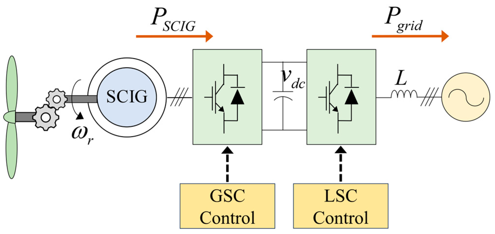
2. SCIG-Based Wind Energy Conversion Systems

2.1. Modeling of SCIG

The model of a SCIG using the d-q components is expressed in the stationary reference frame as [11] (p. 238) and [44]

$$v_{\mathit{ds}}^s=R_s{i}_{\mathit{ds}}^s+\frac{d{\lambda }_{\mathit{ds}}^s}{\mathit{dt}}$$

(1)

$$v_{qs}^s=R_s{i}_{qs}^s+\frac{d{\lambda }_{qs}^s}{\mathit{dt}}$$

(2)

$$0=R_r{i}_{\mathit{dr}}^s+\frac{d{\lambda }_{\mathit{dr}}^s}{\mathit{dt}}+{\omega }_r{\lambda }_{\mathit{qr}}^s$$

(3)

$$0=R_r{i}_{\mathit{qr}}^s+\frac{d{\lambda }_{\mathit{qr}}^s}{\mathit{dt}} -{\omega }_r{\lambda }_{\mathit{dr}}^s$$

(4)

where v_ds and v_qs represent the d- and q-axis components of stator voltage, respectively (V); i_ds and i_qs are the d- and q-axis components of stator current, respectively (A); i_dr and i_qr are the d- and q-axis components of rotor current, respectively (A); ω_r is the rotor shaft angular velocity (rad/s); R_s and R_r are the stator and rotor resistances (Ω), respectively; λ_ds and λ_qs represent the d- and q-axis components of stator flux linkage, respectively (Wb); λ_dr and λ_qr represent the d- and q-axis components of rotor flux linkage, respectively (Wb). The stator and rotor flux linkages in (1)–(4) can be derived as

$${\lambda }_{\mathit{ds}}^s=L_s{i}_{\mathit{ds}}^s+L_m{i}_{\mathit{dr}}^s$$

(5)

$${\lambda }_{\mathit{qs}}^s=L_s{i}_{\mathit{qs}}^s+L_m{i}_{\mathit{qr}}^s$$

(6)

$${\lambda }_{\mathit{dr}}^s=L_m{i}_{\mathit{ds}}^s+L_r{i}_{\mathit{dr}}^s$$

(7)

$${\lambda }_{\mathit{qr}}^s=L_m{i}_{\mathit{qs}}^s+L_r{i}_{\mathit{qr}}^s$$

(8)

where L_m is the magnetizing inductance (H); L_ls and L_lr are the stator and rotor leakage inductances, respectively (H); L_s and L_r are the stator and rotor self-inductances, respectively (H). It is noted that L_s = L_ls + L_m, and L_r = L_lr + L_m.

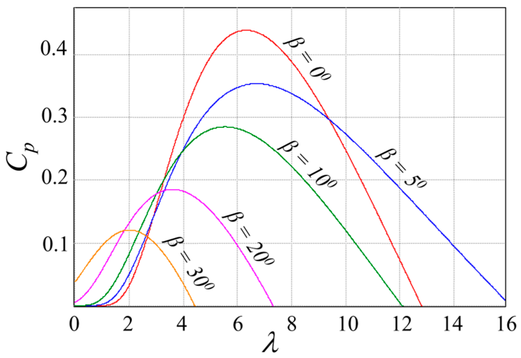
2.2. Modeling of Wind Turbines

The mechanical power P_tur regarded as the output of the wind turbines can be obtained as

$$P_{\mathit{tur}}=0.5\rho A{C}_p\left(\beta ,\lambda \right)V_w^3$$

(9)

where ρ is air density (kg/m³); A is blade swept area (m²); V_w is wind speed (m/s); and C_p (β, λ) is power conversion coefficient determined based on the blade pitch angle β and the tip-speed ratio λ. The tip–speed ratio and power conversion coefficient can be expressed as [45]

$$\lambda =\frac{{\omega }_{t}R}{V_w}$$

(10)

$$C_p\left(\lambda ,\beta \right)=0.22\left[\frac{116}{\mathit{\Lambda }}0.4\beta -5\right]e^{-\frac{12.5}{\mathit{\Lambda }}}$$

(11)

where R is blade radius (m); ω_t is wind turbine shaft angular velocity (rad/s); the factor Λ can be obtained by

$$\frac{1}{\mathit{\Lambda }}=\frac{1}{\lambda +0.08\beta }-\frac{0.035}{1+{\beta }^3}$$

(12)

The power coefficient curves under various conditions of β and λ are illustrated in Figure 1. Since the desired operating points of the wind turbine systems are the ones corresponding to the maximum values of C_p, the maximum power point tracking (MPPT) algorithm, which can ensure that C_p maintains = its optimal values, is commonly used in such systems [46].

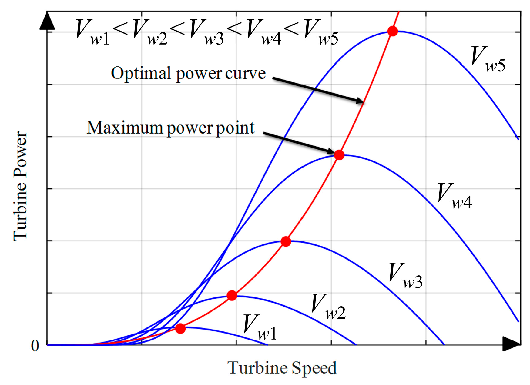
2.3. MPPT Algorithm for Wind Turbine Systems

Figure 2 shows the relationship between turbine power and turbine speed under various conditions of wind speed. The operating points of the wind turbine located in the red curve in Figure 2, i.e., the optimal power curve, are called the maximum power points. The MPPT algorithms for wind turbine systems, which ensure that the operating points of the wind turbine track the maximum power points corresponding to the optimal value of C_p, can be categorized as hill-climb search (HCS) control, tip–speed ratio (TSR) control, and power signal feedback (PSF) control [46]. Although the HCS control is the simplest algorithm among these, its performance can be significantly deteriorated under rapid changes in the wind speed [47]. For the TSR control algorithm, the tip–speed ratio in (10) is adjusted to optimal value by controlling the turbine speed or generator rotor speed to vary with wind speed. Although the TSR control can offer high efficiency and fast response, it requires information on wind speed, which can be obtained using an anerometer, and this makes the system more costly, not to mention that wind speed measurement of the anemometer can be inaccurate due to non-uniformities in wind speed along the length of the blades, as well as before and after passing through turbine blades [48]. It is also important to note with TSR control that regulating the generator rotor speed under rapid changes in wind speed can cause a fast variation in electromagnetic torque, which can adversely affect the mechanical parts of the system. Compared to TSR control, although the PSF control offers lower efficiency, it can provide robustness and cost-effectiveness with no need for the anemometer. Furthermore, for PSF control, setting the reference of generator active power corresponding to the rotor speed based on the optimal power curve depicted in Figure 2 can alleviate the rapid fluctuations in generator torque that may occur with the TSR control algorithm, as well as provide the direct regulation of the amount of active power from the generator to the grid. For the reasons above, the PSF MPPT control is considered for this research.

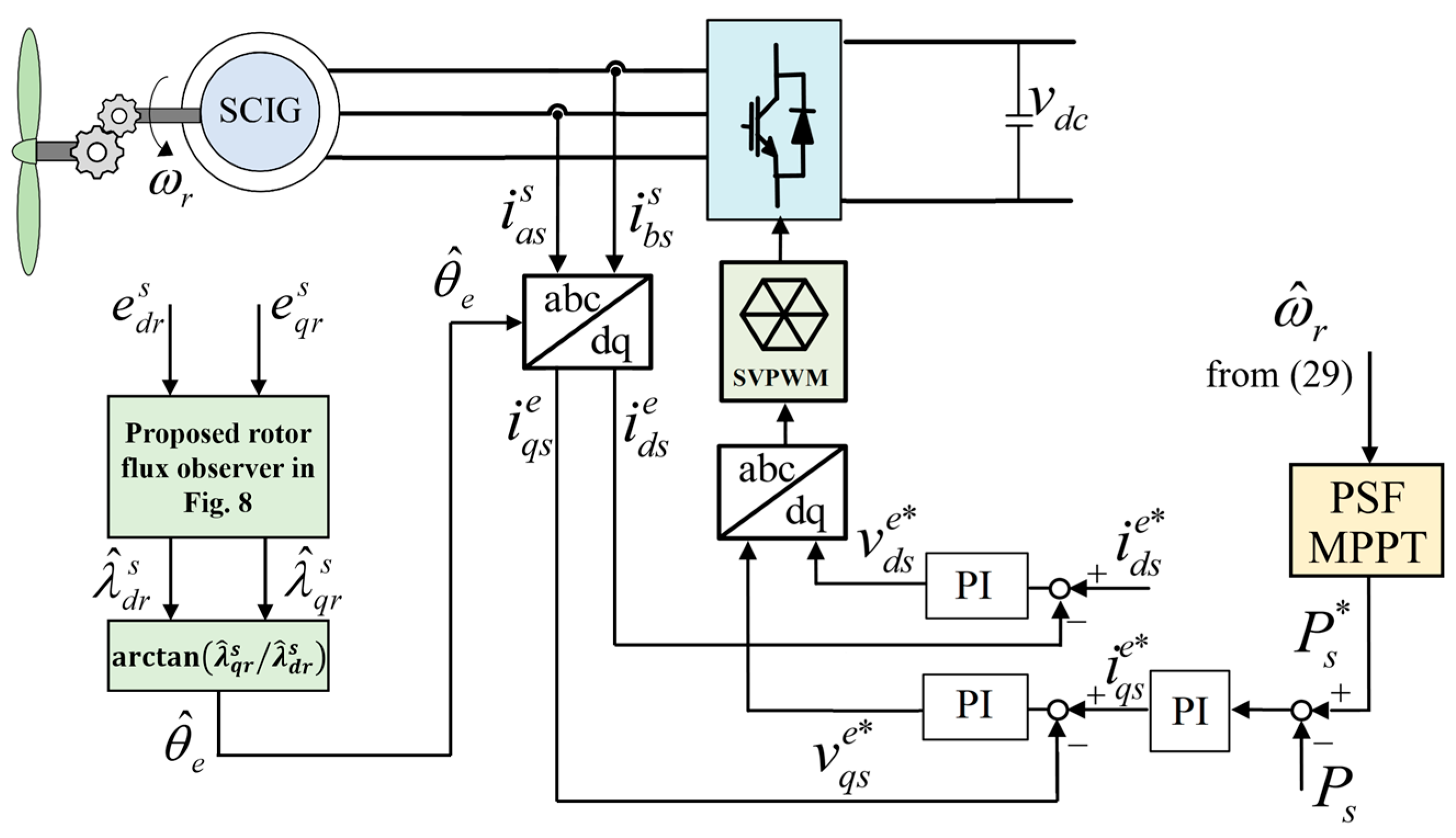
2.4. Control of SCIG-Based Wind Energy Conversion Systems

The configuration of the SCIG-based wind energy conversion system is shown in Figure 3, in which the SCIG is connected to the grid via the back-to-back converter consisting of the generator-side and the line-side converters. Both the generator-side and line-side converters use the cascade control scheme including the two cascaded control loops, of which the inner loop is designed for the current regulation. The PSF MPPT algorithm is realized by the generator-side converter. By regulating the d- and q-axis line-side currents, respectively, the DC-link voltage and power factor can be controlled by the line-side converter.

3. Proposed Sensorless Control Method

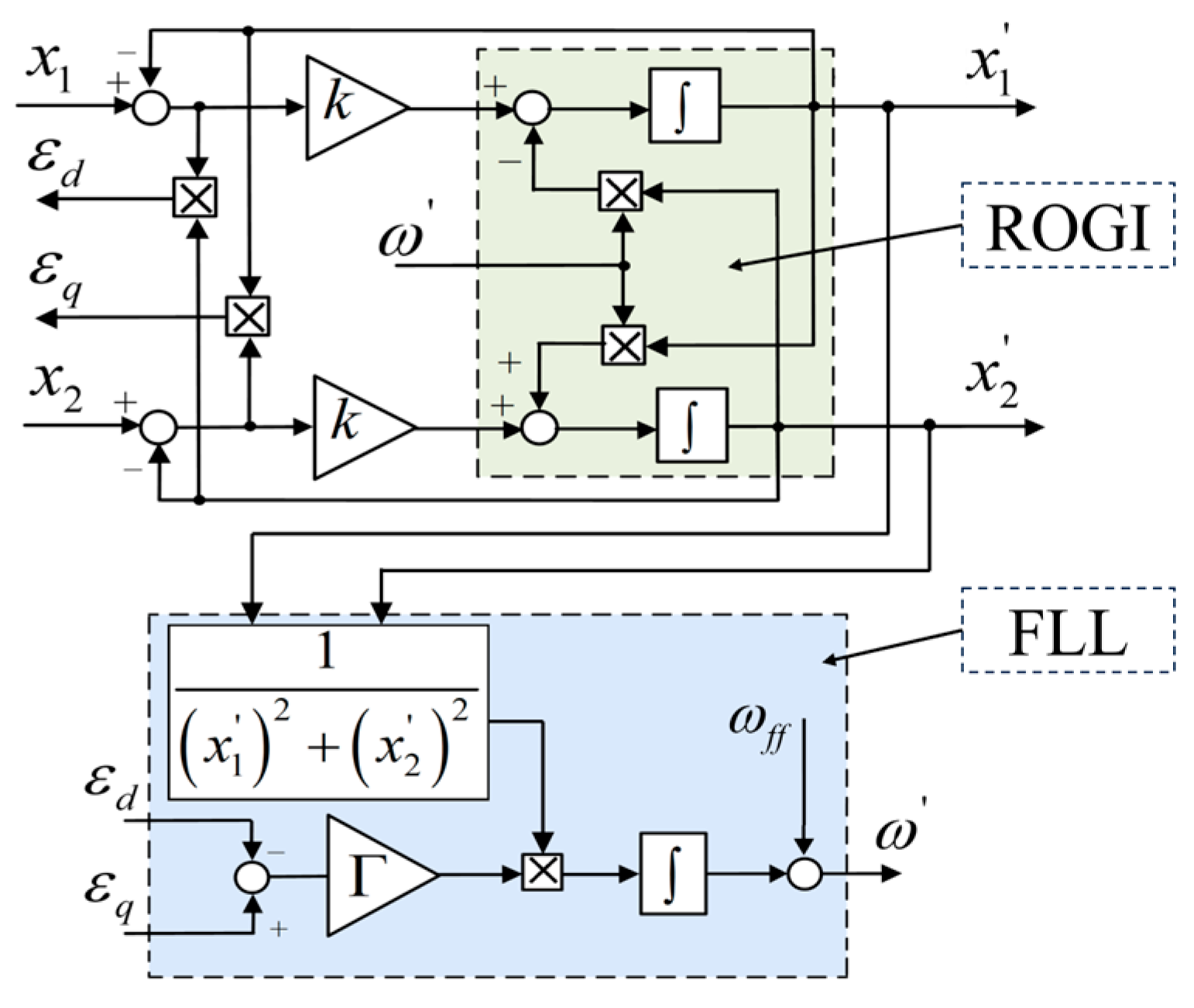
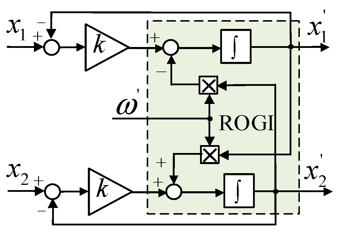
3.1. Standard ROGI Structure

Figure 4 shows the structure of the ROGI-based adaptive filter (AF), in which x₁ and x₂ are the input signals, $x_1\prime$ and $x_2\prime$ are the output signals, k is ROGI gain and $\omega \prime$ is the tuning frequency.

In the stationary reference frame for the three-phase systems, if x₁ and x₂ are the rotating components that are in quadrature with each other, the ROGI-based AF transfer functions can be derived from Figure 4 as [36]

$$G_1\left(s\right)=\frac{x_1\prime }{x_1}=\frac{\mathit{ks}+\left(k^2+\mathit{jk}\omega \prime \right)}{s^2+2\mathit{ks}+\left(k^2+\omega {\prime }^2\right)}$$

(13)

$$G_2\left(s\right)=\frac{x_1\prime }{x_2}=\frac{\mathit{jks}+\left(j{k}^2-k\omega \prime \right)}{s^2+2\mathit{ks}+\left(k^2+\omega {\prime }^2\right)}$$

(14)

$$G_3\left(s\right)=\frac{x_2\prime }{x_1}=\frac{-\mathit{jks}+\left(k\omega \prime -j{k}^2\right)}{s^2+2\mathit{ks}+\left(\omega {\prime }^2+k^2\right)}$$

(15)

$$G_4\left(s\right)=\frac{x_2\prime }{x_2}=\frac{\mathit{ks}+\left(k^2+\mathit{jk}\omega \prime \right)}{s^2+2\mathit{ks}+\left(\omega {\prime }^2+k^2\right)}$$

(16)

From (13)–(16), the relationship between $x_1\prime$ and $x_2\prime$ can be obtained as

$$\frac{x_1\prime }{x_2\prime }=\frac{\mathit{jks}+\left(j{k}^2-k\omega \prime \right)}{\mathit{ks}+\left(k^2+\mathit{jk}\omega \prime \right)}=j$$

(17)

It is worth noting from (17) that $x_1\prime$ and $x_2\prime$ are the two quadrature components, regardless of whether $\omega \prime$ equals the rotational frequency of $x_1\prime$ and $x_2\prime$.

The poles of the ROGI transfer functions can be solved by finding the roots of denominators of (13)–(16) as

$$s_{1,2}=-k \pm j\omega \prime$$

(18)

From (18), it is noted that the stability of ROGI can be guaranteed if k is higher than zero. Moreover, since the real parts of s_1,2 are −k, the settling time of the ROGI response can be approximated as

$$t_{s\left(\mathit{ROGI}\right)}\approx 5/k$$

(19)

From (19), it is worth mentioning that k can be arbitrarily selected to achieve the pre-specified settling time. However, the high value of k can deteriorate the harmonic rejection capability of ROGI.

3.2. ROGI-FLL for Rotor Flux Linkage Estimation

By considering (14) and (15), $x_1\prime$ and $x_2\prime$ can be derived in the time domain as

$$x_1\prime \left(t\right)=\frac{-k^2\omega \left[k^2+{\left(\omega +\omega \prime \right)}^2\right]\int x_2\left(t\right)\mathit{dt}}{\left[k^2+{\left(\omega +\omega \prime \right)}^2\right]\left[k^2+{\left(\omega -\omega \prime \right)}^2\right]}+\frac{x_2\left(t\right)\left[k\left({\omega }^3-\omega {\prime }^3\right)+\left(k^3+k\omega \omega \prime \right)\left(\omega -\omega \prime \right)\right]}{\left[k^2+{\left(\omega +\omega \prime \right)}^2\right]\left[k^2+{\left(\omega -\omega \prime \right)}^2\right]}$$

(20)

$$x_2\prime \left(t\right)=\frac{k^2\omega \left[k^2+{\left(\omega +\omega \prime \right)}^2\right]\int x_1\left(t\right)\mathit{dt}}{\left[k^2+{\left(\omega +\omega \prime \right)}^2\right]\left[k^2+{\left(\omega -\omega \prime \right)}^2\right]}+\frac{x_1\left(t\right)\left[k\left(\omega {\prime }^3-{\omega }^3\right)+\left(k^3+k\omega \omega \prime \right)\left(\omega \prime -\omega \right)\right]}{\left[k^2+{ \left(\omega +\omega \prime \right)}^2\right]\left[k^2+{\left(\omega -\omega \prime \right)}^2\right]}$$

(21)

where ω is the rotational frequency of x₁ and x₂.

With the use of the frequency-locked loop (FLL) structure shown in Figure 5, $\omega \prime$ can be adapted to ω [27]. Hence, (20) and (21) can be re-written under the assumption ω ≈ $\omega \prime$ as follows:

$$x_1\prime \left(t\right)=-\omega \prime \int x_2\left(t\right)\mathit{dt}$$

(22)

$$x_2\prime \left(t\right)=\omega \prime \int x_1\left(t\right)\mathit{dt}$$

(23)

In (22) and (23), if x₁ and x₂ are the rotor EMFs, $e_{\mathit{dr}}^s$ and $e_{\mathit{qr}}^s$, which are found from the mathematical model of SCIG as

$$e_{\mathit{dr}}^s=\frac{L_r\left(\left(v_{\mathit{ds}}^s-R_s{i}_{\mathit{ds}}^s\right)-\sigma L_{s}d{i}_{\mathit{ds}}^s/\mathit{dt}\right)}{L_m}$$

(24)

$$e_{\mathit{qr}}^s=\frac{L_r\left(\left(v_{\mathit{qs}}^s-R_s{i}_{\mathit{qs}}^s\right)-\sigma L_{s}d{i}_{\mathit{qs}}^s/\mathit{dt}\right)}{L_m}$$

(25)

where σ is the leakage factor, defined as $\sigma =1-L_m^2/L_s{L}_r$.

Then, from (22) and (23), the d-q axis rotor flux linkage ${\lambda }_{\mathit{dqr}}^s$ can be estimated from the ROGI outputs, $e_{\mathit{dr}}^s\prime$ and $e_{\mathit{qr}}^s\prime$, as

$${\widehat{\lambda }}_{\mathit{dr}}^s=\frac{e_{\mathit{qr}}^s\prime }{\omega \prime }$$

(26)

$${\widehat{\lambda }}_{\mathit{qr}}^s=-\frac{e_{\mathit{dr}}^s\prime }{\omega \prime }$$

(27)

where the caret “^” represents the estimated value.

Based on (22)–(27), the rotor flux observer using the ROGI-FLL is shown in Figure 6. The estimated rotor flux angle ${\widehat{\theta }}_e$ and rotor speed ${\widehat{\omega }}_r$ can be obtained as

$${\widehat{\theta }}_e=\mathit{arctan}\left({\widehat{\lambda }}_{\mathit{qr}}^s/{\widehat{\lambda }}_{\mathit{dr}}^s\right)$$

(28)

$${\widehat{\omega }}_r={\widehat{\omega }}_e-{\widehat{\omega }}_{\mathrm{sl}}$$

(29)

where ${\widehat{\omega }}_e$ is the estimated synchronous speed and ${\widehat{\omega }}_{\mathrm{sl}}$ is the estimated slip speed given by

$${\widehat{\omega }}_{\mathrm{sl}}=\frac{L_m{R}_r\left({\widehat{\lambda }}_{\mathit{dr}}^s{i}_{\mathit{qs}}^s-{\widehat{\lambda }}_{\mathit{qr}}^s{i}_{\mathit{ds}}^s\right)}{L_r\left({\widehat{\lambda }}_{\mathit{dr}}^{s2}+{\widehat{\lambda }}_{\mathit{qr}}^{s2}\right)}$$

(30)

Theoretically, ${\widehat{\omega }}_e$ in (29) can be determined by taking the derivative of ${\widehat{\theta }}_e$. However, with the utilization of the arctangent function in (28), ${\widehat{\theta }}_e$ can be changed suddenly from π to −π, and this can cause spikes in ${\widehat{\omega }}_e$. To deal with this difficulty, ${\widehat{\omega }}_e$ can be obtained by an estimator, as shown in Figure 7. In the speed estimator depicted in Figure 7, the PI controller gains, k_p and k_i, are selected as 100 and 2000, respectively, corresponding to the bandwidth of 100 rad/s.

It is worth mentioning that with the excellent harmonic rejection capability of ROGI, the rotor flux observer using ROGI-FLL shown in Figure 6 can offer robust estimation performance against switching ripples, electromagnetic noises, sensing circuit noise, etc. In addition, the structure of that observer is simpler than that of the rotor flux observer using dual SOGI-FLL [31].

In the case of the existence of DC offset components, which are mainly caused by the measurement errors or differences in the switching behavior of power devices [49,50,51], in the rotor EMFs in (24) and (25), the DC offset components in the estimated rotor flux linkages in (26) and (27), ${\widehat{\lambda }}_{\mathit{od}}$ and ${\widehat{\lambda }}_{\mathit{oq}}$, can be derived as

$${\widehat{\lambda }}_{\mathit{od}}=\frac{E_{\mathit{od}}k}{\omega \prime \sqrt{k^2+\omega {\prime }^2}}\mathit{sin}\left({\mathit{tan}}^{-1}\frac{\omega \prime }{k}\right)+\frac{E_{\mathit{oq}}k}{\omega \prime \sqrt{k^2+\omega {\prime }^2}}\mathit{cos}\left({\mathit{tan}}^{-1}\frac{\omega \prime }{k}\right)$$

(31)

$${\widehat{\lambda }}_{\mathit{oq}}=\frac{E_{\mathit{oq}}k}{\omega \prime \sqrt{k^2+\omega {\prime }^2}}\mathit{sin}\left({\mathit{tan}}^{-1}\frac{\omega \prime }{k}\right)-\frac{E_{\mathit{od}}k}{\omega \prime \sqrt{k^2+\omega {\prime }^2}}\mathit{cos}\left({\mathit{tan}}^{-1}\frac{\omega \prime }{k}\right)$$

(32)

where E_od and E_oq are the DC offset components in $e_{\mathit{dr}}^s$ and $e_{\mathit{qr}}^s$, respectively.

From (31) and (32), it is noted that the DC offset components in and ${\lambda }_{\mathit{dr}}^s$ are ${\lambda }_{\mathit{qr}}^s$ affected by both E_od and E_oq. Notably, although the negative effects of DC offset components on the rotor flux estimation when using the ROGI-FLL are mitigated compared with when using the dual SOGI-FLL [43], those DC offset components can cause oscillations in estimated rotor speed. As a result, oscillations can exist in the stator active power since the stator active power reference is obtained from a look-up table with the input of estimated rotor speed according to the PSF MPPT algorithm [46].

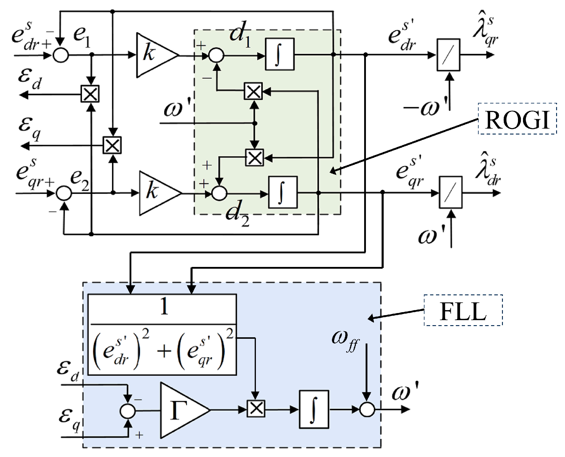
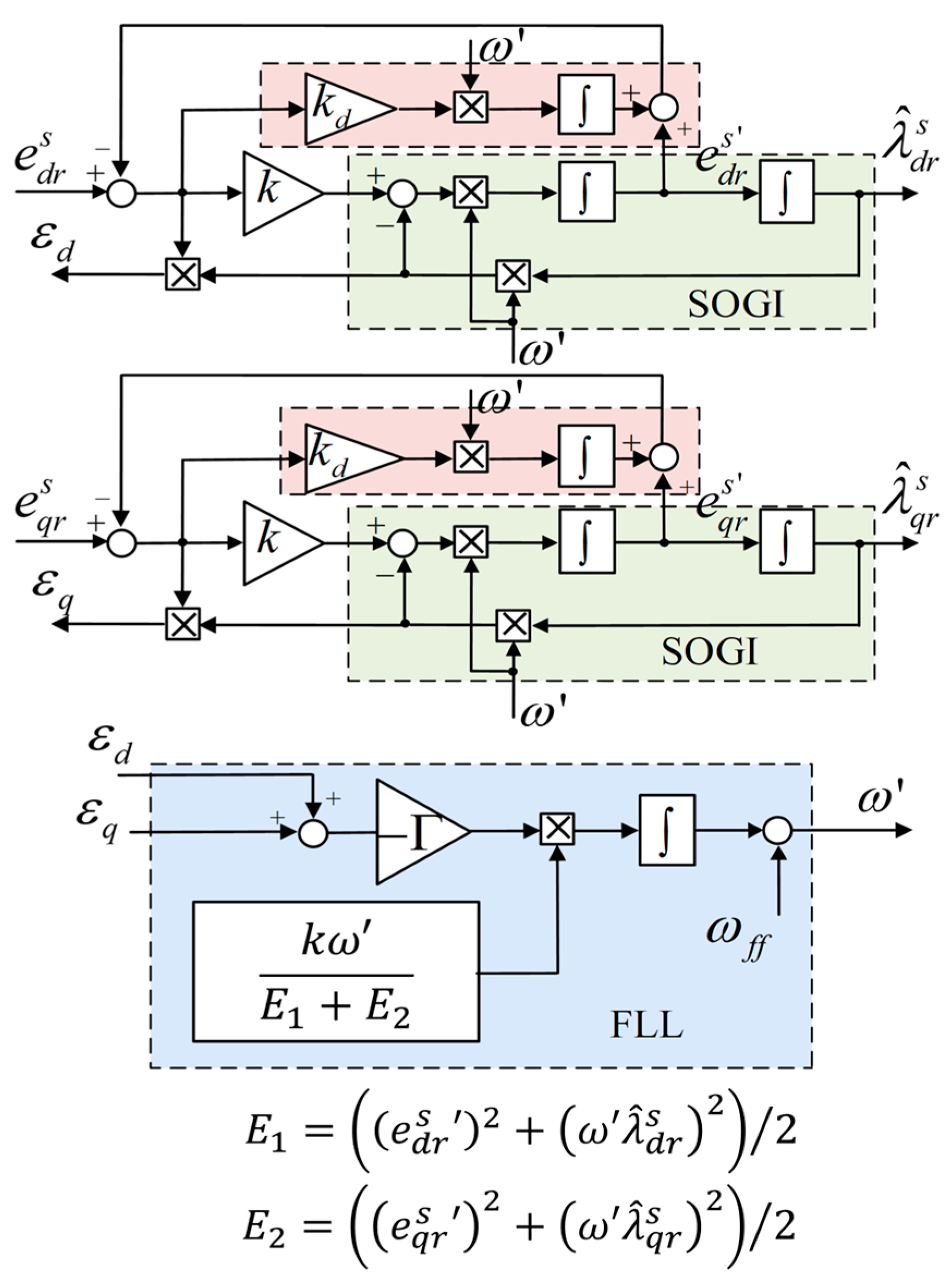
3.3. Modified ROGI-FLL Including DC Offset Compensators for Rotor Flux Linkage Estimation

As mentioned, the DC offset in the estimated rotor flux linkages can negatively affect the system performance. To address this difficulty, a modified ROGI-FLL with DC offset compensator-based rotor flux observers is proposed, as shown in Figure 8. Using the proposed observer, the DC offset components of $e_{\mathit{dr}}^s$ and $e_{\mathit{qr}}^s$ in (24) and (25) can be estimated. After that, the sum of these estimated DC offset components, and the proposed observer outputs are feedbacked to modify the signals e₁ and e₂ in Figure 8. As a result, the DC offset components in $e_{\mathit{dr}}^s\prime$ and $e_{\mathit{qr}}^s\prime$ can be significantly reduced [38,39]. The configuration of the SCIG control system with the proposed observer is shown in Figure 9, in which the PSF MPPT algorithm is implemented by adjusting the generator active power reference to correspond with variations in estimated rotor speed in accordance with the optimal power curve shown in Figure 2.

To help readers better understand the proposed flux observer, thereby making it easier to choose its parameters, the next sub-section of the paper will clarify the influences of the parameters on the dynamic response of the proposed flux observer, for example, settling time of response, harmonic rejection capability, error in $\omega \prime$ under variation in ω_e.

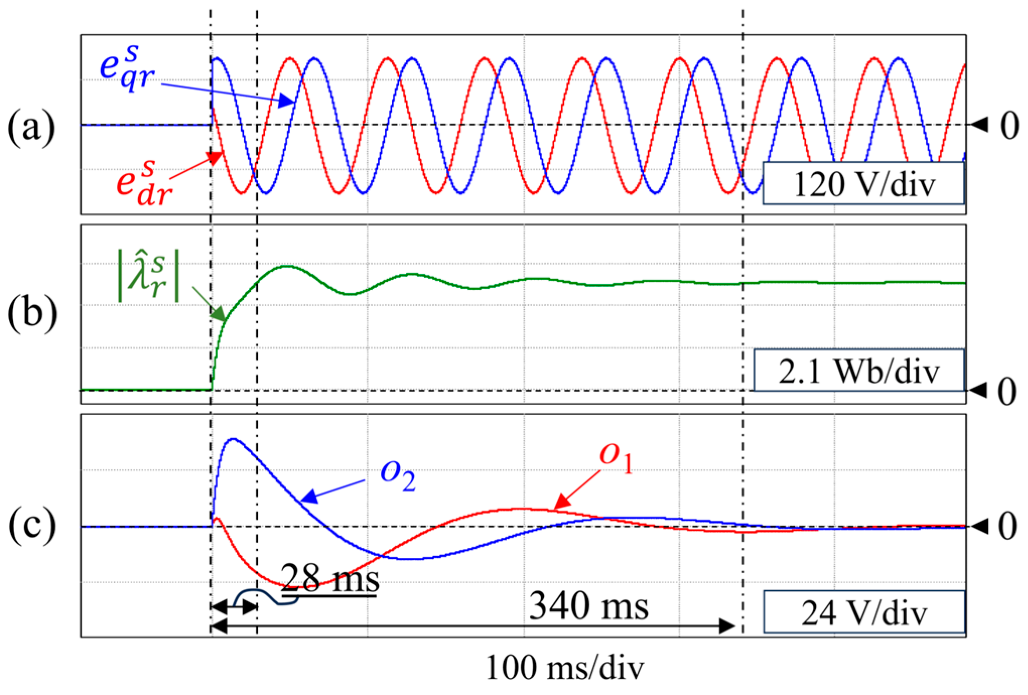
3.4. Dynamic Response Analysis of Proposed Rotor Flux Observer

3.4.1. Influences of k and k_d on Rotor Flux Estimation

In Figure 8, the transfer functions of the proposed rotor flux observer are expressed as

$$G_d\left(s\right)=\frac{e_{\mathit{dr}}^s\prime }{e_{\mathit{qr}}^s}=\frac{{\mathit{jks}}^3+\left(-k\omega \prime +{\mathit{jkA}}_1\right)s^2-k{k}_d{\omega }^{\prime 2}s}{s^4+2A_1{s}^3+\left(A_1^2+{\omega }^{\prime 2}\right)s^2+2k_d{\omega }^{\prime 3}s+k_d^2{\omega }^{\prime 4}}$$

(33)

$$G_q\left(s\right)=\frac{e_{\mathit{qr}}^s\prime }{e_{\mathit{dr}}^s}=\frac{-{\mathit{jks}}^3+\left(k\omega \prime -{\mathit{jkA}}_1\right)s^2+k{k}_d{\omega }^{\prime 2}s}{s^4+2A_1{s}^3+\left(A_1^2+{\omega }^{\prime 2}\right)s^2+2k_d{\omega }^{\prime 3}s+k_d^2{\omega }^{\prime 4}}$$

(34)

where A₁ = $\left(k+k_d\omega \prime \right)$, and k_d is the gain of the DC offset compensators.

Figure 10 shows the frequency responses of (33) and (34) in terms of magnitude under various conditions of k and k_d when $\omega \prime$ is 2π50 rad/s. It is worth mentioning that the frequency responses at the frequencies below $\omega \prime$ are affected by both k_d and k, whereas those at the frequencies above $\omega \prime$ are only affected by k. Furthermore, Figure 10 shows that the magnitude of the DC offset components in the proposed observer outputs are significantly reduced as k_d increases.

Four poles of G_d(s) and G_q(s) in (33) and (34) are defined as

$$s_{1,2}=-a \pm \mathit{jb}$$

(35)

$$s_{3,4}=-c \pm \mathit{jd}$$

(36)

where a, b, c, and d are positive real numbers. If k_d in (33) and (34) is set to zero, the poles s_3,4 are eliminated. In other words, s_3,4 occur due to the employment of the DC offset compensators.

In (35) and (36), for the value of a to be equal to the value of c, the selection of k and k_d should meet the following requirements:

$$k=k_d\omega \prime$$

(37)

$$4k^2\le \omega {\prime }^2$$

(38)

Then, the a, b, c, and d in (35) and (36) can be expressed as

$$a=c=k$$

(39)

$$b=\sqrt{\frac{\omega {\prime }^2-2k^2+\omega \prime \sqrt{\omega {\prime }^2-4k^2}}{2}}$$

(40)

$$d \sqrt{\frac{\omega {\prime }^2-2k^2-\omega \prime \sqrt{\omega {\prime }^2-4k^2}}{2}}$$

(41)

The settling time of ROGI output, in this case, can be approximated as

$$t_{s\left(\mathit{ROGI}\right)}\approx \frac{5}{a}$$

(42)

For example, k and k_d are selected as 157 and 0.5, respectively, $\omega \prime$ is locked to 2π50 rad/s, and hence, the requirements in (37) and (38) are met. Figure 11 shows the performance of rotor flux linkage estimation using the proposed observer. The EMFs $e_{\mathit{dr}}^s$ and $e_{\mathit{qr}}^s$ are shown in Figure 11a. In Figure 11b,c, the amplitude $\left|{\widehat{\lambda }}_r^s\right|$, i.e., $\sqrt{{\left({\widehat{\lambda }}_{\mathit{dr}}^s\right)}^2+{\left({\widehat{\lambda }}_{\mathit{qr}}^s\right)}^2}$, and the estimated DC offsets, i.e., o₁ and o₂, are shown, respectively. Note that for Figure 11 and other figures illustrating the waveforms of quantities from now on, the names of the waveforms in each sub-figure will be shown in the figure caption, and the scale of the horizontal axis representing the time is placed at the bottom of the figure, while the scale of vertical axis representing the value is placed in the lower right corner of each sub-figure. As seen in Figure 11b, the setting time of response of $\left|{\widehat{\lambda }}_r^s\right|$ is about 35 ms, which is similar to the results obtained by (42), i.e., t_s(ROGI) ≈ 32 ms. Under another operating condition, the performance of rotor flux linkage estimation in the presence of the DC offset in ${ e}_{\mathit{dqr}}^s$ (10% of rotor EMF amplitude) is shown in Figure 12. Similar to that of Figure 11, the settling time of response of $\left|{\widehat{\lambda }}_r^s\right|$ is about 35 ms, as shown in Figure 12b.

Figure 13 shows the root loci of (33) and (34) in response to different values of $\omega \prime$ which can be significantly varied during the operation of the system. As aforementioned, with k and k_d of 157 and 0.5 are selected, respectively, the requirements in (37) and (38) can be met if $\omega \prime$ is 2π50 rad/s. In this case, the real parts of poles of (33) and (34), i.e., a and c in (35) and (36), are the same, as derived in (39). If $\omega \prime$ is not 2π50 rad/s, and the requirements in (37) and (38) are not met; these real parts are different from each other, as shown in Figure 13. Therefore, it can be said that the values of a, b, c, and d in (35) and (36) are not always obtained by (39)–(41) due to the variation in $\omega \prime$.

From Figure 13, for the cases in which $\omega \prime$ is not 2π50 rad/s, it is worth mentioning that the rotor flux observer output responses to any changes in its inputs ${ e}_{\mathit{dqr}}^s$ consists of two portions, they are fast and slowly changing portions corresponding to the settling times t_{s(ROGI_fast)} and t_{s(ROGI_slow)}, respectively, which are approximated as

$$t_{s\left(\mathit{ROGI}\_\mathit{fast}\right)}\approx 5/A_2$$

(43)

$$t_{s\left(\mathit{ROGI}\_\mathit{slow}\right)}\approx 5/C_2$$

(44)

where

$$A_2 \approx k+k_d\omega \prime -C_2$$

(45)

$$C_2 \approx \frac{k_d^3\omega {\prime }^5-3k_d^{2}k\omega {\prime }^4+k_d\omega {\prime }^3{C}_1}{k_d^4\omega {\prime }^4-4k_d^{3}k\omega {\prime }^3+2k_d^2\omega {\prime }^2\left(2k^2+C_1\right)-4k_{d}k\omega \prime C_1+C_1^2}$$

(46)

with $C_1=\left(k^2+\omega {\prime }^2\right)$.

For example, k and k_d are selected as 157 and 0.5, respectively, similarly to that in Figure 11, and $\omega \prime$ is locked to 2π16 rad/s. As seen in Figure 14b, the response of $\left|{\widehat{\lambda }}_r^s\right|$ consists of fast and slowly changing portions corresponding to the settling times of 28 ms and 340 ms, respectively, which are similar to results obtained by (45) and (46), i.e., t_{s(ROGI_fast)} ≈ 26 ms and t_{s(ROGI_slow)} ≈ 333 ms.

In the steady-state operation, the proposed observer outputs, $e_{\mathit{dr}}^s\prime$ and $e_{\mathit{qr}}^s\prime$, can be derived as

$$e_{\mathit{dr}}^s\prime =\mathit{Ecos}\left({\omega }_{e}t\right)+{\sum }_{h=2}^{\infty }{\zeta }_h{E}_h\mathit{cos}\left(h{\omega }_{e}t+\mathit{arctan}{\theta }_h\right)$$

(47)

$$e_{\mathit{qr}}^s\prime =\mathit{Esin}\left({\omega }_{e}t\right)+{\sum }_{h=2}^{\infty }{\zeta }_h{E}_h\mathit{sin}\left(h{\omega }_{e}t+\mathit{arctan}{\theta }_h\right)$$

(48)

where E and E_h are the fundamental and harmonic component amplitudes of $e_{\mathit{dqr}}^s\prime$, respectively, and h is the harmonic order of $e_{\mathit{dqr}}^s\prime$. The coefficient ζ_h and angle θ_h are expressed as

$${\zeta }_h=k/\sqrt{k^2+{\left(\omega \prime -h{\omega }_e\right)}^2}$$

(49)

$${\theta }_h=\left(\omega \prime -h{\omega }_e\right)$$

(50)

From (49) and (50), it is worth mentioning that although k can be arbitrarily selected to meet the pre-specified requirements of the settling time of responses, the high value of k can deteriorate the harmonic rejection capability of the ROGI, and this can be seen in Figure 10a as well. Moreover, in (47) and (48), the harmonic components are not affected by k_d, as shown in Figure 10b as well.

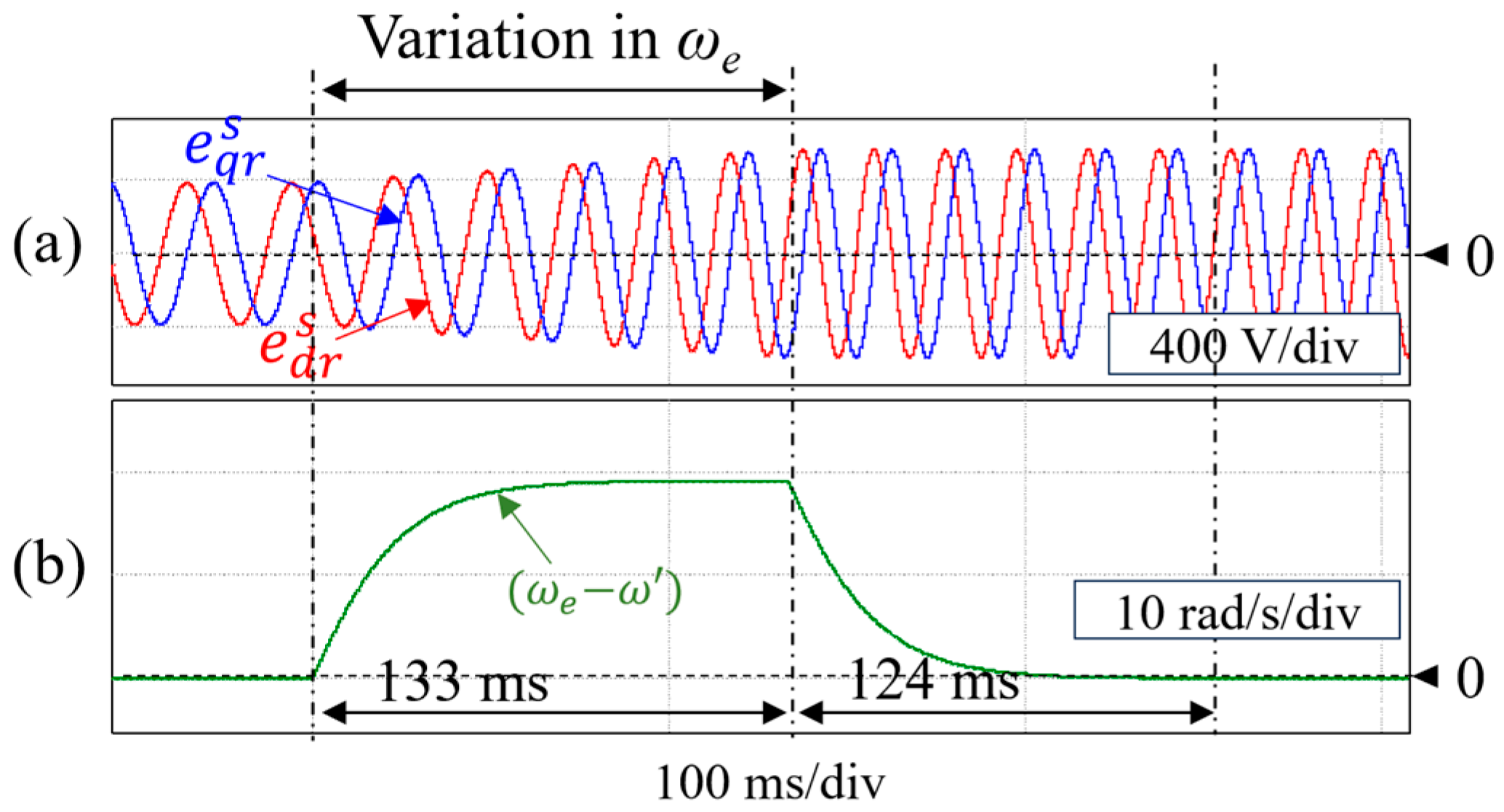
3.4.2. Influence of Г on Rotor Flux Estimation

Under operations with ${\dot{\omega }}_e\approx 0$, assuming that $\omega \prime$ approximates ω_e and DC offset component of ROGI outputs are significantly compensated, the errors e₁ and e₂ in Figure 8 can be derived as

$$e_1\approx e_{\mathit{qr}}^s\prime \left(\omega \prime {-\omega }_e\right)/k$$

(51)

$$e_2\approx e_{\mathit{dr}}^s\prime \left({\omega }_e-\omega \prime \right)/k$$

(52)

For the FLL structure in Figure 8, $\dot{\omega }\prime$ can be expressed as

$$\frac{\left(e_2{e}_{\mathit{dr}}^s\prime -e_1{e}_{\mathit{qr}}^s\prime \right)\mathsf{\Gamma }}{{\left(e_{\mathit{dr}}^s\prime \right)}^2+{\left(e_{\mathit{qr}}^s\prime \right)}^2}=\dot{\omega }\prime$$

(53)

From (51) and (52), (53) can be re-written as

$$-\left(\omega \prime {-\omega }_e\right)\mathsf{\Gamma }/k=\dot{\omega }\prime$$

(54)

Then, the transfer function of FLL can be obtained from (54) as

$$\frac{\omega \prime \left(s\right)}{{\omega }_e\left(s\right)}=\frac{\mathsf{\Gamma }/k}{s+\mathsf{\Gamma }/k}$$

(55)

where k/Г is the time constant corresponding to the settling time of the FLL response, which can be derived as

$$t_{s\left(\mathit{FLL}\right)}\approx 5k/\mathsf{\Gamma }$$

(56)

Assuming that there is a variation in the synchronous speed Δ_ω within the duration Δ_t, the ramp input r_in(t) and ramp response r_res(t) of the FLL based on (55) are obtained as [52]

$$r_{\mathit{in}}\left(t\right)={\Delta }_{\omega }t/{\Delta }_t$$

(57)

$$r_{\mathit{res}}\left(t\right)=\left({\Delta }_{\omega }t/{\Delta }_t-{\Delta }_{\omega }k/\left({\Delta }_t\mathsf{\Gamma }\right)\right)+{\Delta }_{\omega }k/\left({\Delta }_t\mathsf{\Gamma }\right)e^{-\mathsf{\Gamma }t/k}$$

(58)

It is worth mentioning that the time constant of FLL should be high enough to that of ROGI with a DC offset compensator. Therefore, in this work, k = 157 and k_d = 0.5 are selected, corresponding to the ROGI time constant of 6.4 ms at a tuning frequency of 2π50 rad/s, and Г = 6160 is selected, corresponding to the FLL time constant of 25.5 ms. In Figure 15, ω_e is varied from 2π34 rad/s to 2π50 rad/s within 133 ms. From (58), the tuning frequency estimation error Δ_ωk/(Δ_tГ) is about 19.3 rad/s, which approximates the simulation result, i.e., 19.2 rad/s, as shown in Figure 15b. It is observed that after the actual value of ω_e reaches the steady-state value of 2π50 rad/s at t = t₂, the settling time of the FLL response is about 124 ms, which is similar to the result obtained from (56), i.e., 127 ms.

It can be noted that Δ_ωk/(Δ_tГ) always exists under variations in ω_e, as shown in Figure 15. However, since the stator frequency is estimated based on ${\widehat{\theta }}_e$, as shown in Figure 7, this estimation error Δ_ωk/(Δ_tГ) does not nearly affect the rotor speed estimation performance.

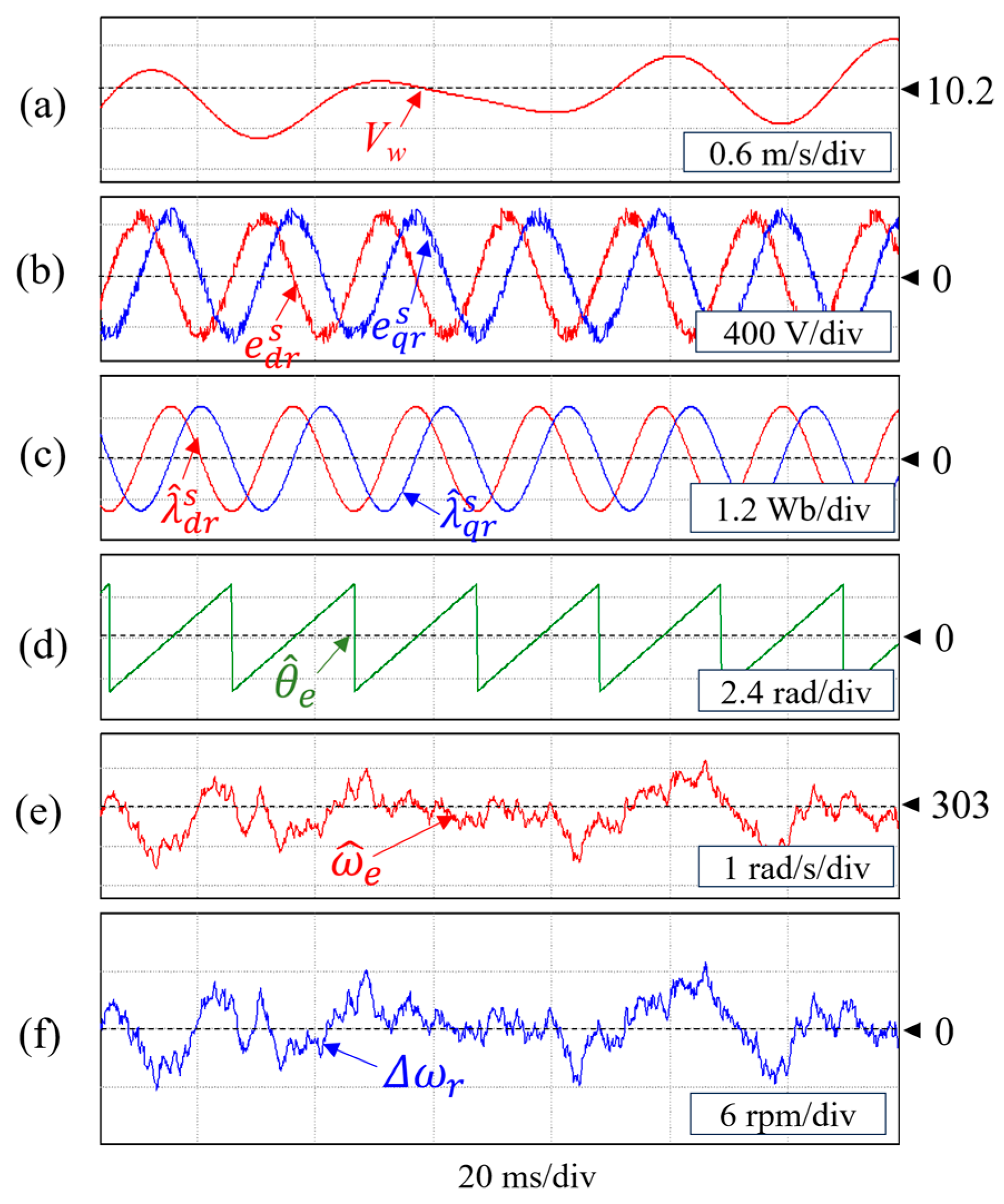
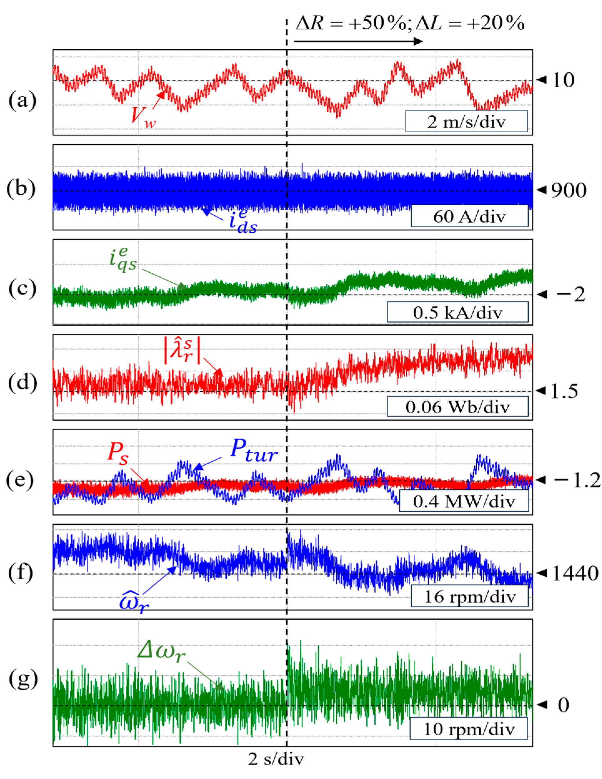
4. Results and Discussion

In the PSIM platform, a simulation system with a power rating of 2 MW, of which the specifications are listed in

Table 1. Parameters of SCIG.

Parameters	Values
Stator frequency	50 Hz
Rated stator power	2 MW
Rated line–line stator voltage	690 V
Rated stator current	2000 A
Pole pairs	2
Stator resistance	1.102 mΩ
Magnetizing inductance	2.1346 mH
Stator leakage inductance	0.0649 mH
Rated speed	1520 rpm

and

Table 2. Wind turbine specification.

Parameters	Values
Rated power	2 MW
Blade radius	45 m
Gear ratio	1:123
Cut-in/Cut-off speed	4 m/s~25 m/s
Rated wind speed	12 m/s
Operating speed range	675 rpm~1500 rpm

, is built to verify the effectiveness of the proposed method. The DC link voltage is controlled to 1200 V. The switching frequency is 5 kHz.

For the parameters of the ROGI-FLL with the DC compensators, k = 157 and k_d = 0.5 are selected to achieve t_s(ROGI) = 32 ms at the operation stator frequency of 50 Hz, and Г = 6160 is selected corresponding to t_s(FLL) = 127 ms.

Figure 16 shows the performance of the rotor flux linkage estimation in response to wind speed fluctuation using the proposed flux observer. The wind speed pattern is shown in Figure 16a. It is noted that the negative effects of high-frequency components in rotor EMFs in Figure 16b on the estimated rotor flux linkages can be significantly reduced, as shown in Figure 16c. The estimated rotor flux linkage angle and synchronous angular velocity are illustrated in Figure 16d and Figure 16e, respectively. Figure 16f shows the error in rotor shaft speed estimation, which is relatively small (about 0.4% of the actual speed).

In this work, the performance comparison between the proposed method and the dual SOGI-FLL with DC offset compensator-based method, of which the rotor flux observer is shown in Figure 17, is conducted. To achieve similar settling times to those of ROGI-FLL, the parameters of dual SOGI-FLL, i.e., k, k_d, and Г, are set to 1, 0.272, and 19.7, respectively, corresponding to t_s(SOGI) = 32 ms at the operation stator frequency of 50 Hz and t_s(FLL) = 127 ms.

The sensorless control performance when subjected to wind speed fluctuation, which can cause the variation in wind turbine torque and parameter mismatch using the existing method based on dual SOGI-FLL with DC offset compensators [32] is shown in Figure 18. Under this operating condition, the variations in the SCIG parameters, i.e., ΔR = +50% and ΔL = +20%, are considered. Figure 18a depicts the wind speed pattern. The d-axis stator current is controlled to 890 A, whereas the q-axis stator current is regulated to obtain the desired active power regarding the MPPT algorithm, as shown in Figure 18b and Figure 18c, respectively. Figure 18d illustrates the amplitude of the estimated rotor flux linkage. As can be seen in Figure 18e,f, when the magnitude of SCIG active power is greater than that of a wind turbine, the rotor shaft speed is decreased and vice versa. The average error in speed estimation is about 7 rpm (0.48% of rotor shaft speed) in the presence of variation in SCIG parameters, as shown in Figure 18g. It is noted that since this existing method is based on the model, the effects of parameter mismatch are inevitable. However, the adverse effects of this deviation on SCIG wind turbine system performance can be negligible, as evidenced by the fact that it can be seen no significant changes in q-axis stator current and stator active power controls when the parameter mismatch begins to occur in Figure 18c and Figure 18e, respectively.

Figure 19 depicts the sensorless control performance when subjected to wind speed fluctuation and parameter mismatch using the proposed method. It can be noted from Figure 18 and Figure 19 that there is no significant difference between the system performances using the existing method in [32] and the proposed method. However, as the computational burden of ROGI-FLL is less than that of dual SOGI-FLL [43] when the proposed method is used, there is the execution of a greater number of tasks within one sampling period compared to when the existing method in [32] is used. This can enable system performance improvement as well as the reduced requirement for the number of digital signal processors (DSP) when handling similar workloads. It is worth mentioning that if there is no DC offset in derived rotor EMFs, the performance of the proposed method and that of the existing method based on ROGI-FLL in [43] are almost similar to each other.

In the presence of stator voltage disturbance, the sensorless control performances when using the existing methods based on dual SOGI-FLL and ROGI-FLL [31,43] are shown in Figure 20 and Figure 21, respectively. In this case, the DC offset of 10% of the rated stator phase voltage, i.e., 56 V, is considered, which is intentionally added to the phase-A stator voltage reference in the software code. In Figure 20d, it is observed that the maximum error in speed estimation corresponding to the dual SOGI-FLL-based method is about 40 rpm, whereas that corresponding to the ROGI-FLL-based method is only about 20 rpm, as shown in Figure 21d. This difference in the speed estimation error comes from the difference in the behavior of the gain characteristics of the transfer functions of dual SOGI-FLL- and ROGI-FLL-based observers at the frequency of zero [43]. But no matter what, these errors are quite large, and they can cause oscillations in the SCIG active power due to the MPPT algorithm.

Figure 22 and Figure 23 illustrate the sensorless control performances in the presence of stator voltage disturbance when using the existing method based on dual SOGI-FLL with DC offset compensation in [32] and the proposed method, respectively. It can be seen in Figure 22d and Figure 23d, with the use of a DC offset compensator, the oscillations in the speed estimation errors caused by the DC offset in rotor EMFs are remarkably reduced, leading to reducing the oscillations in the SCIG stator active power, as the power signal feedback MPPT method is used. This not only increases system efficiency but also reduces mechanical stresses on the rotating shaft, which can be caused by oscillations in SCIG electromagnetic torque. As a result, the lifespans of SCIG and gearbox systems can be increased, also the maintenance and operational costs can be decreased. As observed from Figure 22d and Figure 23d, the maximum value of error in speed estimation using the proposed method is about 12 rpm (0.83% of rotor shaft speed), and it is lower than that using the existing method based on dual SOGI-FLL with DC offset compensator, i.e., about 33 rpm (2.27% of rotor shaft speed). Therefore, it can be said that in this case, there is superiority of the proposed method over the existing method [32] in reducing the speed estimation error.

Since the rotor EMFs derived from the machine modeling are regarded as input of the proposed rotor flux observer, the suggested sensorless control method faces challenges starting from zero speed when there is no information on rotor EMFs. To address this challenge, the V/f method is employed during the startup phase while the rotor flux linkage angle is estimated but it is not used for the sensorless control yet. Once the estimated rotor shaft speed reaches a predetermined minimum speed, such as 200 rpm [11] (pp. 298–299) [43], the estimated rotor flux linkage angle becomes the basis for coordinate transformation, and the MPPT algorithm is initiated.

Despite the starting issue mentioned above, the proposed sensorless control method is entirely suitable for the SCIG wind turbine systems employing full-scale power converters since the typical operating speed range of such systems is usually from 45% to 100% of the rated speed. Moreover, the proposed rotor flux observer can also be developed with slight modifications for permanent magnet synchronous generator wind turbine systems utilizing full-scale power converters, where the field flux phase angle is needed for sensorless control. However, for doubly fed induction generator wind turbine systems using partial-scale power converters, the proposed rotor flux observer cannot be applied, although there has been a study of utilization of dual SOGI structure for rotor position estimation in such systems [53].

As shown in Figure 3, the GSC is connected to the grid via the LSC and DC-link capacitor. Therefore, grid disturbances directly affect the performance of the LSC without causing major impacts on the performance of the GSC. In other words, despite grid disturbances, the effectiveness of ROGI-FLL, including DC offset compensators-based flux estimation for SCIG active power control, is almost unchanged compared to the normal working conditions.

From the above analysis of the relationship between the dynamic response and parameters of the proposed rotor flux observer, it can be said that the design of such an observer is not dependent on the power rating of the system but on the specific requirements related to the dynamic response of rotor flux observer.

Since the proposed sensorless control method with the V/f starting method only makes changes in the software and does not modify the hardware, it can theoretically be applied to any existing SCIG wind turbine systems with the three-phase voltage-source PWM converter. However, this application needs to be carefully considered as it relates to the specific operating procedures of each SCIG wind turbine system, which have been verified and issued by the manufacturer, for example, acceleration during the startup phase, rotation speed for beginning applying the estimated rotor flux angle, how to handle a converter fault, etc.

5. Conclusions

In this paper, the improved sensorless control scheme, including the MPPT algorithm for grid-connected SCIG wind turbine systems, is proposed. This method utilizes the rotor flux linkage observer based on modified ROGI-FLL with DC offset compensation capability. The ROGI-FLL, known for its excellent harmonic rejection capability, can enhance the robustness of rotor flux linkage estimation by effectively handling high-frequency components. Moreover, the DC offset compensators combined with the ROGI-FLL play a pivotal role in reducing the DC offset component in the estimated rotor flux linkages. This reduction is crucial as the DC offset can induce oscillations in the estimated rotor shaft speed, consequently causing oscillations in SCIG active power when the MPPT algorithm is applied.

To validate the proposed method, a 2 MW SCIG wind turbine simulation system has been built. Via the verification results, it is noted that the average error in the speed estimation in the presence of parameter mismatch, i.e., ΔR = +50% and ΔL = +20%, when using the proposed method is about 7 rpm (0.48% of rotor shaft speed), and there are no serious effects on the system performance caused by this error. In addition, despite the stator voltage disturbance of 10% of rated stator phase voltage, i.e., 56 V, the DC offset component in the estimated rotor flux linkages almost does not exist owing to the DC offset compensation. As a result, the oscillation in the SCIG active power is significantly mitigated.

Conducting the comparison of the proposed method using the modified ROGI-FLL with DC offset compensators with an existing method using the dual SOGI-FLL with DC offset compensators in [32], the advantages of the proposed method have been highlighted. The proposed method demonstrates a simpler structure, thereby reducing the required number of DSPs as well as having the potential to improve system performance. Additionally, under stator voltage disturbance, the proposed method can yield a lower speed estimation error, approximately 1.44% less than the existing method in [32].

It is worth noting that the expected performance of the proposed method cannot be achieved when faults caused by the failures of power electronic switching devices occur, for example, open-circuit switch faults. Hence, it is crucial to address the challenges associated with such faults, which will be investigated in future studies, to enhance the reliability of the speed sensorless control method for SCIG systems.

References

1. Renewables 2020 Global Status Report. 2020. Available online: https://www.ren21.net/wp-content/uploads/2019/05/gsr_2020_full_report_en.pdf (accessed on 4 March 2024).
2. Maktabi, M.; Rusu, E. A review of perspectives on developing floating wind farms. Inventions 2024, 9, 24. [Google Scholar] [CrossRef]
3. Luo, J.; Bu, S.; Zhu, J. A Novel PMU-based adaptive coordination strategy to mitigate modal resonance between full converter-based wind generation and grids. IEEE J. Emerg. Sel. Top. Power Electron. 2021, 9, 7173–7182. [Google Scholar] [CrossRef]
4. Beik, O.; Al-Adsani, A.S. A wind turbine generator design and optimization for DC collector grids. IEEE J. Emerg. Sel. Top. Power Electron. 2022, 10, 484–493. [Google Scholar] [CrossRef]
5. Song, G.; Cao, B.; Chang, L. Advanced soft stall control for protection of small-scale wind generation systems. IEEE J. Emerg. Sel. Top. Power Electron. 2022, 10, 273–284. [Google Scholar] [CrossRef]
6. Bashetty, S.; Ozcelik, S. Design and stability analysis of an offshore floating multi-wind turbine platform. Inventions 2022, 7, 58. [Google Scholar] [CrossRef]
7. Aissou, R.; Rekioua, T.; Rekioua, D.; Tounzi, A. Robust nonlinear predictive control of permanent magnet synchronous generator turbine using Dspace hardware. Int. J. Hydrogen Energy 2016, 41, 21047–21056. [Google Scholar] [CrossRef]
8. Telsnig, T. Wind Energy Technology Development Report 2020-EUR 30503 EN; Publications Office of the European Union: Luxembourg, 2020; ISBN 978-92-76-27273-1. [Google Scholar]
9. Thoroughly Tested, Utterly Reliable. Available online: https://pdf.archiexpo.com/pdf/siemens-gamesa/swt-36-120/88089-134487.html (accessed on 4 March 2024).
10. Yaramasu, V.; Wu, B.; Sen, P.; Kouro, S.; Narimani, M. High-power wind energy conversion systems: State-of-the-art and emerging technologies. Proc. of the IEEE 2015, 103, 740–788. [Google Scholar] [CrossRef]
11. Sul, S.-K. Control of Electric Machine Drive Systems; John Willey & Sons: Hoboken, NJ, USA, 2011. [Google Scholar]
12. Caruana, C.; Asher, G.M.; Sumner, M. Performance of HF signal injection techniques for zero-low-frequency vector control of induction machines under sensorless conditions. IEEE Trans. Ind. Electron. 2006, 53, 225–238. [Google Scholar] [CrossRef]
13. Yoon, Y.-D.; Sul, S.-K. Sensorless control for induction machines based on square-wave voltage injection. IEEE Trans. Power Electron. 2014, 29, 3637–3645. [Google Scholar] [CrossRef]
14. Holtz, J.; Quan, J. Drift- and parameter-compensated flux estimator for persistent zero-stator-frequency operation of sensorless-controlled induction motors. IEEE Trans. Ind. Appl. 2003, 39, 1052–1060. [Google Scholar] [CrossRef]
15. Das, S.; Kumar, R.; Pal, A. MRAS-based speed estimation of induction motor drive utilizing machines’ d- and q-circuit impedances. IEEE Trans. Ind. Electron. 2019, 66, 4286–4295. [Google Scholar] [CrossRef]
16. Hinkkanen, M.; Harnefors, L.; Luomi, J. Reduced-order flux observers with stator-resistance adaptation for speed-sensorless induction motor drives. IEEE Trans. Power Electron. 2010, 25, 1173–1183. [Google Scholar] [CrossRef]
17. Zaky, M.S.; Metwaly, M.K. Sensorless torque/speed control of induction motor drives at zero and low frequencies with stator and rotor resistance estimations. IEEE J. Emerg. Sel. Top. Power Electron. 2016, 4, 1416–1429. [Google Scholar] [CrossRef]
18. Alonge, F.; Cangemi, T.; D’Ippolito, F.; Fagiolini, A.; Sferlazza, A. Convergence analysis of extended Kalman filter for sensorless control of induction motor. IEEE Trans. Ind. Electron. 2015, 62, 2341–2352. [Google Scholar] [CrossRef]
19. Zhang, X. Sensorless induction motor drive using indirect vector controller and sliding-mode observer for electric vehicles. IEEE Trans. Veh. Technol. 2013, 62, 3010–3018. [Google Scholar] [CrossRef]
20. Hu, J.; Wu, B. New integration algorithms for estimating motor flux over a wide speed range. IEEE Trans. Power Electron. 1998, 13, 969–977. [Google Scholar]
21. Comanescu, M.; Xu, L. An improved flux observer based on PLL frequency estimator for sensorless vector control of induction motors. IEEE Trans. Ind. Electron. 2006, 53, 50–56. [Google Scholar] [CrossRef]
22. Bose, B.K.; Patel, N.R. A programmable cascaded low-pass filter-based flux synthesis for a stator flux-oriented vector-controlled induction motor drive. IEEE Trans. Ind. Electron. 1997, 44, 140–143. [Google Scholar] [CrossRef]
23. Shin, M.-H.; Hyun, D.-S.; Cho, S.-B.; Choe, S.-Y. An improved stator flux estimation for speed sensorless stator flux orientation control of induction motors. IEEE Trans. Power Electron. 2000, 15, 312–318. [Google Scholar] [CrossRef]
24. Hackl, C.M.; Landerer, M. Modified second-order generalized integrators with modified frequency locked loop for fast harmonics estimation of distorted single-phase signals. IEEE Trans. Power Electron. 2020, 35, 3298–3309. [Google Scholar] [CrossRef]
25. Matas, J.; Castilla, M.; Miret, J.; De Vicuña, L.G.; Guzman, R. An adaptive prefiltering method to improve the speed/accuracy tradeoff of voltage sequence detection methods under adverse grid conditions. IEEE Trans. Ind. Electron. 2014, 61, 2139–2151. [Google Scholar] [CrossRef]
26. Rodríguez, P.; Luna, A.; Candela, I.; Mujal, R.; Teodorescu, R.; Blaabjerg, F. Multiresonant frequency-locked loop for grid synchronization of power converters under distorted grid conditions. IEEE Trans. Ind. Electron. 2011, 58, 127–138. [Google Scholar] [CrossRef]
27. Rodríguez, P.; Luna, A.; Muñoz-Aguilar, R.S.; Etxeberria-Otadui, I.; Teodorescu, R.; Blaabjerg, F. A stationary reference frame grid synchronization system for three-phase grid-connected power converters under adverse grid conditions. IEEE Trans. Power Electron. 2012, 27, 99–112. [Google Scholar] [CrossRef]
28. Sreejith, R.; Singh, B. Sensorless predictive current control of PMSM EV drive using DSOGI-FLL based sliding mode observer. IEEE Trans. Ind. Electron. 2021, 68, 5537–5547. [Google Scholar] [CrossRef]
29. Kashif, M.; Murshid, S.; Singh, B. Solar PV array fed self-sensing control of PMSM drive with robust adaptive hybrid SOGI based flux observer for water pumping. IEEE Trans. Ind. Electron. 2021, 68, 6962–6972. [Google Scholar] [CrossRef]
30. Dao, N.D.; Lee, D.-C.; Lee, S.-M. A simple and robust sensorless control based on stator current vector for PMSG wind power systems. IEEE Access 2018, 7, 8070–8080. [Google Scholar] [CrossRef]
31. Xin, Z.; Zhao, E.; Blaabjerg, F.; Zhang, L.; Loh, P.C. An improved flux observer for field-oriented control of induction motors based on dual second-order generalized integrator frequency-locked loop. IEEE J. Emerg. Sel. Top. Power Electron. 2017, 5, 513–525. [Google Scholar] [CrossRef]
32. Zhao, R.; Xin, Z.; Loh, P.C.; Blaabjerg, F. A novel flux estimator based on multiple second-order generalized integrators and frequency-locked loop for induction motor drives. IEEE Trans. Power Electron. 2017, 32, 6286–6296. [Google Scholar] [CrossRef]
33. Xu, W.; Jiang, Y.; Mu, C.; Blaabjerg, F. Improved nonlinear flux observer-based second-order SOIFO for PMSM sensorless control. IEEE Trans. Power Electron. 2019, 34, 565–579. [Google Scholar] [CrossRef]
34. Harnefors, L.; Hinkkanen, M. Complete stability of reduced-order and full-order observers for sensorless IM drives. IEEE Trans. Ind. Electron. 2008, 55, 1319–1329. [Google Scholar] [CrossRef]
35. Harnefors, L.; Ottersten, R. Regeneration-mode stabilization of the ‘statically compensated voltage model. IEEE Trans. Ind. Electron. 2007, 54, 818–824. [Google Scholar] [CrossRef]
36. Xin, Z.; Zhao, R.; Mattavelli, P.; Loh, P.C.; Blaabjerg, F. Re-investigation of generalized integrator based filters from a first-order system perspective. IEEE Access 2016, 4, 7131–7144. [Google Scholar] [CrossRef]
37. Golestan, S.; Guerrero, J.M.; Vasquez, J.C. Is using a complex control gain in three-phase FLLs reasonable? IEEE Trans. Ind. Electron. 2020, 67, 2480–2484. [Google Scholar] [CrossRef]
38. Karimi-Ghartemani, M.; Khajehoddin, S.A.; Jain, P.K.; Bakhshai, A.; Mojiri, M. Addressing DC component in PLL and notch filter algorithms. IEEE Trans. Power Electron. 2012, 27, 78–86. [Google Scholar] [CrossRef]
39. Wang, A.J.; Ma, B.Y.; Meng, C.X. A frequency-locked loop technology of three-phase grid-connected inverter based on improved reduced-order generalized integrator. In Proceedings of the 2015 IEEE 10th Conference on Industrial Electronics and Applications, Auckland, New Zealand, 15–17 June 2015; pp. 730–735. [Google Scholar]
40. Golestan, S.; Guerrero, J.M.; Vasquez, J.; Abusorrah, A.M.; Al-Turki, Y.A. A study on three-phase FLLs. IEEE Trans. Power Electron. 2019, 34, 213–224. [Google Scholar] [CrossRef]
41. Vazquez, S.; Sanchez, J.A.; Reyes, M.R.; Leon, J.I.; Carrasco, J.M. Adaptive vectorial filter for grid synchronization of power converters under unbalanced and/or distorted grid conditions. IEEE Trans. Ind. Electron. 2014, 61, 1355–1367. [Google Scholar] [CrossRef]
42. Busada, C.A.; Jorge, S.G.; Leon, A.E.; Solsona, J.A. Current controller based on reduced order generalized integrators for distributed generation systems. IEEE Trans. Ind. Electron. 2012, 59, 2898–2909. [Google Scholar] [CrossRef]
43. Nguyen, A.T.; Lee, D.-C. Sensorless control of variable-speed SCIG wind energy conversion systems based on rotor flux estimation using ROGI-FLL. IEEE J. Emerg. Sel. Top. Power Electron. 2022, 10, 7786–7796. [Google Scholar] [CrossRef]
44. Rekioua, D.; Rekioua, T.; Idjdarene, K.; Tounzi, A. An approach for the modeling of an autonomous induction generator taking into account the saturation effect. Int. J. Emerg. Electr. Power Syst. 2005, 4. [Google Scholar] [CrossRef]
45. Yin, M.; Li, G.; Zhou, M.; Zhao, C. Modelling of the wind turbine with permanent magnet synchronous generator for integration. In Proceedings of the 2007 IEEE Power Engineering Society General Meeting, Tampa, FL, USA, 24–28 June 2007; pp. 1–6. [Google Scholar]
46. Thongam, J.S.; Ouhrouche, M. MPPT control methods in wind energy conversion systems. In Fundamental and Advanced Topics in Wind Power; Carriveau, R., Ed.; InTech: Houston, TX, USA, 2011; pp. 339–360. [Google Scholar]
47. Apata, O.; Oyedokun, D. An overview of control techniques for wind turbine systems. Sci. Afr. 2020, 10, e00566. [Google Scholar] [CrossRef]
48. Kumar, D.; Chatterjee, K. A review of conventional and advanced MPPT algorithms for wind energy systems. Renew. Sustain. Energy Rev. 2016, 55, 957–970. [Google Scholar] [CrossRef]
49. Macan, M.; Bahun, I.; Jakopovíc, Ž. Output DC voltage elimination in PWM converters for railway applications. In Proceedings of the 17th International Conference on Electrical Drives and Power Electronics, The High Tatras, Slovakia, 28–30 September 2011; pp. 49–54. [Google Scholar]
50. Long, B.; Zhang, M.; Liao, Y.; Huang, L.; Chong, K.T. An overview of DC component generation, detection and suppression for grid-connected converter systems. IEEE Access 2019, 7, 110426–110438. [Google Scholar] [CrossRef]
51. Zhang, H.; Eng, J. DC Component Elimination at Output Voltage of PWM Inverters. U.S. Patent 7 830 682 B2, 9 November 2010. [Google Scholar]
52. Franklin, G.F.; Powell, J.D.; Emami-Naeini, A. Feedback Control of Dynamic Systems, 6th ed.; Prentice-Hall: Englewood Cliffs, NJ, USA, 2009. [Google Scholar]
53. Nguyen, A.T.; Lee, D.-C. Sensorless control of DFIG wind turbine systems based on SOGI and rotor position correction. IEEE Trans. Power Electron. 2021, 36, 5486–5495. [Google Scholar] [CrossRef]
Figure 1. λ-Cp curves under various conditions of β.
Inventions 09 00044 g001
Figure 2. Turbine power–turbine speed curves under various conditions of wind speed (blue curves) and optimal power curve (red curve).
Inventions 09 00044 g002
Figure 3. Configuration of SCIG-based wind energy conversion system.
Inventions 09 00044 g003
Figure 4. ROGI−based adaptive filter.
Inventions 09 00044 g004
Figure 5. ROGI–FLL–based adaptive filter.
Inventions 09 00044 g005
Figure 6. ROGI-FLL–based rotor flux linkage observer.
Inventions 09 00044 g006
Figure 7. Synchronous speed estimator.
Inventions 09 00044 g007
Figure 8. Modified ROGI-FLL with DC offset compensator-based rotor flux observer.
Inventions 09 00044 g008
Figure 9. Configuration of GSC control with proposed rotor flux observer.
Inventions 09 00044 g009
Figure 10. Frequency responses of Gd(s) and Gq(s) in terms of magnitude (a) with various values of k at kd = 0.1 and (b) with various values of kd at k = 100.
Inventions 09 00044 g010
Figure 11. Rotor flux estimation performance: (a) d-q axis rotor EMF (V); (b) estimated d-q axis rotor flux linkage and its amplitude (Wb); (c) estimated DC offsets of rotor EMF (V).
Inventions 09 00044 g011
Figure 12. Rotor flux estimation performance in the presence of DC offset in rotor EMF (10% of rotor EMF amplitude): (a) d-q axis rotor EMF (V); (b) Estimated d-q axis rotor flux linkage and its amplitude (Wb); (c) Estimated DC offsets of rotor EMF (V).
Inventions 09 00044 g012
Figure 13. Locations of poles of (33) and (34) in response to various values of ω .
Inventions 09 00044 g013
Figure 14. Rotor flux estimation performance for synchronous frequency of 16 Hz: (a) d-q axis rotor EMF (V); (b) amplitude of estimated rotor flux linkage (Wb); (c) estimated DC offsets of rotor EMF (V).
Inventions 09 00044 g014
Figure 15. Tuning frequency estimation performance: (a) d-q-axis rotor EMFs (V); (b) Tuning frequency estimation error (rad/s).
Inventions 09 00044 g015
Figure 16. Rotor flux linkage estimation performance in response to wind speed fluctuation: (a) wind speed (m/s); (b) d-q axis rotor EMFs (V); (c) estimated rotor flux linkages (Wb); (d) estimated rotor flux angle (rad); (e) estimated synchronous speed (rad/s); (f) rotor speed estimation error (rpm).
Inventions 09 00044 g016
Figure 17. Dual SOGI-FLL with DC offset compensator-based rotor flux observer.
Inventions 09 00044 g017
Figure 18. Sensorless control performance when subjected to wind speed fluctuation and parameter mismatch using an existing method based on dual SOGI-FLL with DC offset compensator [32]: (a) wind speed (m/s); (b) d-axis stator current (A); (c) q-axis stator current (A); (d) amplitude of estimated rotor flux linkages (Wb); (e) stator active power and turbine power (W); (f) estimated rotor speed (rpm); (g) rotor speed estimation error (rpm).
Inventions 09 00044 g018
Figure 19. Sensorless control performance when subjected to wind speed fluctuation and parameter mismatch using the proposed method: (a) wind speed (m/s); (b) d-axis stator current (A); (c) q-axis stator current (A); (d) amplitude of estimated rotor flux linkages (Wb); (e) stator active power and turbine power (W); (f) estimated rotor speed (rpm); (g) rotor speed estimation error (rpm).
Inventions 09 00044 g019
Figure 20. Sensorless control performance in the presence of stator voltage disturbance when using an existing method based on dual SOGI-FLL [31]: (a) d-q axis rotor EMFs (V); (b) estimated rotor flux linkages (Wb); (c) amplitude of estimated rotor flux linkages (Wb); (d) rotor speed estimation error (rpm).
Inventions 09 00044 g020
Figure 21. Sensorless control performance in the presence of stator voltage disturbance when using an existing method based on ROGI-FLL [43]: (a) d-q axis rotor EMFs (V); (b) estimated rotor flux linkages (Wb); (c) amplitude of estimated rotor flux linkages (Wb); (d) rotor speed estimation error (rpm).
Inventions 09 00044 g021
Figure 22. Sensorless control performance in the presence of stator voltage disturbance when using dual SOGI-FLL-based method with DC offset compensation [32]: (a) d-q axis rotor EMFs (V); (b) estimated rotor flux linkages (Wb); (c) amplitude of estimated rotor flux linkages (Wb); (d) rotor speed estimation error (rpm).
Inventions 09 00044 g022
Figure 23. Sensorless control performance in the presence of stator voltage disturbance when using the proposed method: (a) d-q axis rotor EMFs (V); (b) estimated rotor flux linkages (Wb); (c) amplitude of estimated rotor flux linkages (Wb); (d) rotor speed estimation error (rpm).
Inventions 09 00044 g023