
Open-Source Design and Economics of Manual Variable-Tilt Angle DIY Wood-Based Solar Photovoltaic Racking System


1
Department of Civil & Environmental Engineering, Western University, London, ON N6A 3K7, Canada
2
Department of Electrical & Computer Engineering, Western University, London, ON N6A 3K7, Canada
3
Ivey School of Business, Western University, London, ON N6A 3K7, Canada
*
Author to whom correspondence should be addressed.
Designs 2022, 6(3), 54; https://doi.org/10.3390/designs6030054
Submission received: 11 May 2022
/
Revised: 6 June 2022
/
Accepted: 9 June 2022
/
Published: 14 June 2022
(This article belongs to the Topic Building Energy and Environment)
Abstract
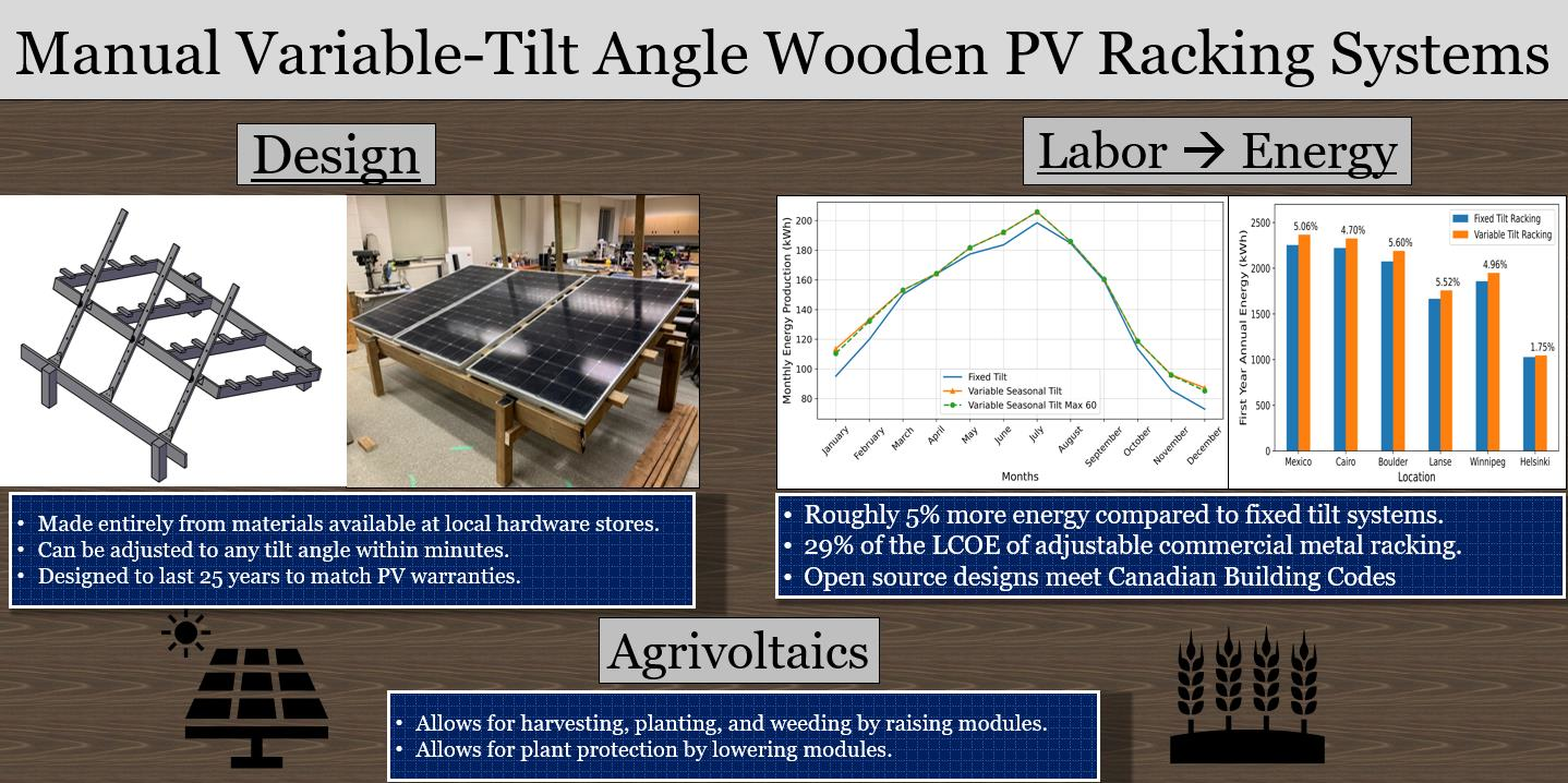
:Fixed-tilt mechanical racking, consisting of proprietary aluminum extrusions, can dominate the capital costs of small-scale solar photovoltaic (PV) systems. Recent design research has shown that wood-racking can decrease the capital costs of small systems by more than 75% in North America. To determine if wood racking provides enough savings to enable labor to be exchanged profitably for higher solar electric output, this article develops a novel variable tilt angle open-source wood-based do-it-yourself (DIY) PV rack that can be built and adjusted at exceptionally low costs. A detailed levelized cost of electricity (LCOE) production analysis is performed after the optimal monthly tilt angles are determined for a range of latitudes. The results show the racking systems with an optimal variable seasonal tilt angle have the best lifetime energy production, with 5.2% more energy generated compared to the fixed-tilt system (or 4.8% more energy, if limited to a maximum tilt angle of 60°). Both fixed and variable wooden racking systems show similar LCOE, which is only 29% of the LCOE of commercial metal racking. The results of this study indicate that the novel variable tilt rack, whether used as a small-scale DIY project or scaled up to fulfill larger energy demands, provides both the lowest cost option even when modest labor costs are included and also may provide specific advantages for applications such as agrivoltaics.
1. Introduction
Solar photovoltaic (PV) technology is a well-established distributed sustainable energy technology [1]. There have been massive PV price declines in the last decade [2,3], which have reduced the levelized cost of electricity (LCOE) [4] to generally be the least-cost option on a large scale [5,6]. In turn, this has made PV the most rapidly expanding electricity generation source (notably the former dominant source, coal is in decline) [6,7]. Worldwide dominance of solar PV as a source of electricity continues to be an economic cost [8]. There is some evidence that at least part of this economic barrier continues to be the focus on large-scale PV deployments [9]. This is despite the fact that small solar home systems can play an important role in achieving the U.N.’s ‘Sustainable Energy for All’ goals [10]. For grid-tied PV systems that have a lower LCOE than the retail rate of grid electricity (e.g., surpassing grid parity), there is massive interest among consumers because they can save money with lower-cost solar electricity [11]. This is particularly true if real net metering is maintained (where prosumers are credited an equivalent economic amount for the electricity they use and send to the grid even if it is not the full value of solar electricity) [12]. Despite clear lifetime economic benefits, the capital expenditures (CAPEX) of PV systems can be challenging for many non-wealthy consumers, both in developing [13] and developed countries [14].
Historically, large-scale centralized PV costs were lower than small-scale distributed costs, and this type of growth continues to dominate the market [9]. The use of small open-source do-it-yourself (DIY) or plug-and-play solar [15,16] has lower costs per unit power than possible for large-scale systems [17]. Among residential systems in the U.S., 8–10 kW systems were roughly 16% less expensive than 2–4 kW systems, and non-residential systems over 1000 kW were 43% less expensive than systems under 10 kW [18]. This small-scale approach deserves appropriate regulation [16,19,20,21] as it could have a substantial economic impact [22]. (Part of the reason small-scale PV systems can be more economic than large-scale industrial PV deployments is that DIY or plug-and-play systems avoid most of the soft costs associated with PV systems. They still have a large CAPEX for many individuals (e.g., even with a ~9-year simple payback period for PV systems under warranty for 25 years that provide an internal rate of return in the double digits, some consumers cannot afford to buy 9 years of electricity upfront even if they receive ‘free’ electricity for another 16 years or more)).
The majority of PV system cost declines have focused on the modules themselves (historically the largest component cost), but now the relative cost of the balance of systems (BOS) made up of racking, electronics, and wiring has become more important [3,23,24]. For the smallest systems, the simple mechanical racking, made up of various proprietary and costly aluminum extrusion profiles that have barely reduced costs [25], can dominate the cost of a whole system. For example, PV module spot prices are currently USD 0.19/W [26], so three 400 W modules cost USD 228 while a three-module rack costs USD 535 (list price USD 635) [27] (e.g., ~2× the cost of the PV) and a three-module pole mount is selling for USD 1194 [28] (e.g., ~5× the cost of the PV).
To combat the distorted market for small-scale PV systems, there has recently been several open-source hardware-based PV racks described, including low-tilt angle arrays, small-scale mobile PV arrays [29], cable-based systems for flat roofs [30], ground-mounted systems at the equator in the developing world [31], tensegrity structures [32], and post-market building-integrated PV (BIPV) [33]. These are all fixed-tilt systems, which are common for industrial PV. This is because simply cleaning large-scale systems can cost anywhere from USD 15 to USD 35 per module [34], so additional labor-intensive work, such as adjusting the tilt of multiple arrays, may be cost-prohibitive. A system in Ontario that is manually adjusted to the optimal tilt angle twice a year generates revenue of USD 1.90 per module each year [35]. All of these systems are fixed-tilt, based on the assumption in the large-scale PV industry that it does not make economic sense to pay people to seasonally adjust the tilt angle of modules. Manual variable-tilt small-scale PV systems exist but have high racking costs and are limited in availability. Therefore, historically, it has generally not been worth hiring personnel to adjust tilt angles. Is this still true, however, if the CAPEX of racking can be radically reduced? More recently, a fixed-tilt wood-based PV DIY rack showed decreases in costs between 49% and 77% compared to proprietary small-scale metal racks [36].
To determine if there has been a shift in the economics of manual tilt adjustment for PV with lower-cost racking, this article develops a variable tilt angle open-source wood-based PV rack following the evolution of the design in [36]. The complete designs and bill of materials (BOM) of the variable tilt angle rack are provided along with basic instructions and are released with an open-source license that will enable anyone to fabricate this rack in their community. A detailed energy production analysis is performed after the optimal monthly tilt angles are determined for a case study location, London, Ontario. The economic analysis accounts for the cost of wood, purchased locally. Then a careful study of the energy production of DIY tilt angle adjustment is run over sensitivity of tilts per year. The energy analysis and economics analysis are combined to evaluate the levelized cost of electricity (LCOE) of the multi-tilt wood racking. The LCOE of the multi-tilt wood racking is then compared to the LCOE of fixed-tilt wood racking, fixed-tilt commercial metal racking, and single-axis tracking commercial metal racking. A sensitivity analysis is then run on the maximum achieved tilt angle as well as the labor cost involved in building the system. The results of this study are discussed in the context of upending the assumption that large scale leads to better economic performance when using open-source DIY design for increasing PV deployments.
2. Materials and Methods
All variables in this report adopt the same abbreviations from Appendix A of the [36] design.
2.1. Material Properties
Construction-grade pressure-treated lumber and hardware purchased from typical hardware stores were used for this design. Material properties from the design in [36] were used for the build of this system. The resisting capacities of each of the wooden members can be calculated by following Appendix A of the design in [36]. Throughout the structural analysis of this design, the limitations outlined in [36] shall not be exceeded.
2.2. Material Stability
Most softwoods are natural organic material subject to deterioration under high moisture conditions, making them an inadequate building material for outdoor use. Some species of wood, such as mahogany and redwood, can naturally fight against decay but are too expensive to be used for outdoor structural use. The best alternative is pressure-treated SPF (Spruce, Pine, Fir) lumber, which offers effective moisture resistance, high availability, and low costs, thus making it an ideal material for structural use in wet climates. Pressure-treated lumber can last upwards of 40 years depending on the moisture conditions [37], making it suitable to use for PV modules with a warranty and expected life of 25 years.
Metal racks are also subject to material degradation that shorten their lifespan due to cross-sectional rusting and corrosion under moist conditions. To account for degradation, engineers apply specified resistance factors that reduce the capacities of both metal and wood structures based on material imperfections under wet conditions. The resistance factors for steel and aluminum are outlined in their respective engineering design handbooks, and the resistance factors for wood are detailed in Appendix A of the design in [36]. Compared to steel and aluminum, wood is a much weaker material, meaning that thicker structural members are required to carry the same loads. Therefore, by designing around the factored capacities of pressure-treated wood, it is possible to design a wooden rack to stand as long as a metal rack under the same weather conditions by building with larger structural wooden members. It should be noted, however, that it makes the most economic sense to only design a rack to match most modules’ warranty and an approximate lifetime of 25 years.
2.3. Energy and Economic Analysis
The energy production analysis of the system is performed using the System Model Advisor (SAM) software [38,39]. A base model is created in SAM with the parameters in Table 1 for a multi-tilt system located in London, Ontario, Canada. A comparative analysis is run between the multi-tilt wood rack in this study and the fixed-tilt wood rack proposed by [36]. The purpose of the energy simulation is to determine the optimal energy production of the system if the tilt angle is adjusted with varying time steps throughout the year. Therefore, a first simulation is run to determine the best tilt angle for each month of the year. To find the best simulation parameters, all the parameters in Table 1 are maintained, except the value of the tilt angle, which is varied from 0° to 90°. The resulting hourly energy production for the first year is aggregated by month and for each tilt angle. The dependence of the maximum monthly energy production on the tilt angle is then analyzed to determine the best tilt angle for each month. The best monthly tilt angles are then used as seasonal tilt angle parameters to determine the lifetime energy production of the system.
Three different energy simulation scenarios are analyzed. The first scenario considers that the racking system is adjusted monthly using the optimal angles. The second scenario explores the case where the maximum angle that can be reached is 60°. In the second scenario, any month with a tilt angle greater than 60° is capped at 60°. As a result, in the case of London, Ontario, the tilt angles of January, February, November, and December are set to 60° instead of the values. Lastly, the third case scenario is the optimal yearly fixed tilt angle (34°), as analyzed by [36].
A detailed economic analysis based on the bill of materials is conducted. The cost of the multi-tilt wood racking system is based on local purchases, and since the system is a DIY system, the labor cost is not factored into the base case study. The lifetime energy production of the PV system and the cost of the racking is used to determine the levelized cost of electricity (LCOE) of the multi-tilt wood racking system, which is then compared to the LCOE structural BOS in fixed-tilt wood racking, commercial fixed-tilt metal racking, and commercial single-axis tracking metal racking. As the system is designed to be DIY and only the racking cost is being analyzed, the discount factor is not included in the calculation of the LCOE (see Equation (1)).
Finally, sensitivity analyses are conducted to assess the power output and system cost in different regions of the world. Simulations are run for multiple locations with various latitudes to determine if a user in different regions can yield the same technical benefit. Furthermore, the cost of pressure-treated wood in different countries is compared to determine if this system can truly provide an economic benefit outside of Canada.
2.4. Design Analysis Assumptions
The same design analysis assumptions from the design in [36] were used for this system, including the specified snow, wind, and total design load.
3. Results
3.1. Bill of Materials
The bill of materials (BOM) of the multi-tilt system is shown in Table 2 in Canadian dollars sourced from Copp’s Build-All and The Home Depot, London.
The modules used for this racking design are LG 400 W NeON2 modules. The approximate dimensions of the modules are 1 × 2 m. If modules with different dimensions are to be used, then the specifications in the assembly instructions in Section 3.2 can be scaled up or down to fulfill the given module size requirements. Resizing the system will change the loads applied to the wood, which means smaller systems reduce costs by selecting smaller structural members such that no limits are exceeded when conducting the structural analysis outlined in Appendix A.
3.2. Variable Angle Installation Instructions
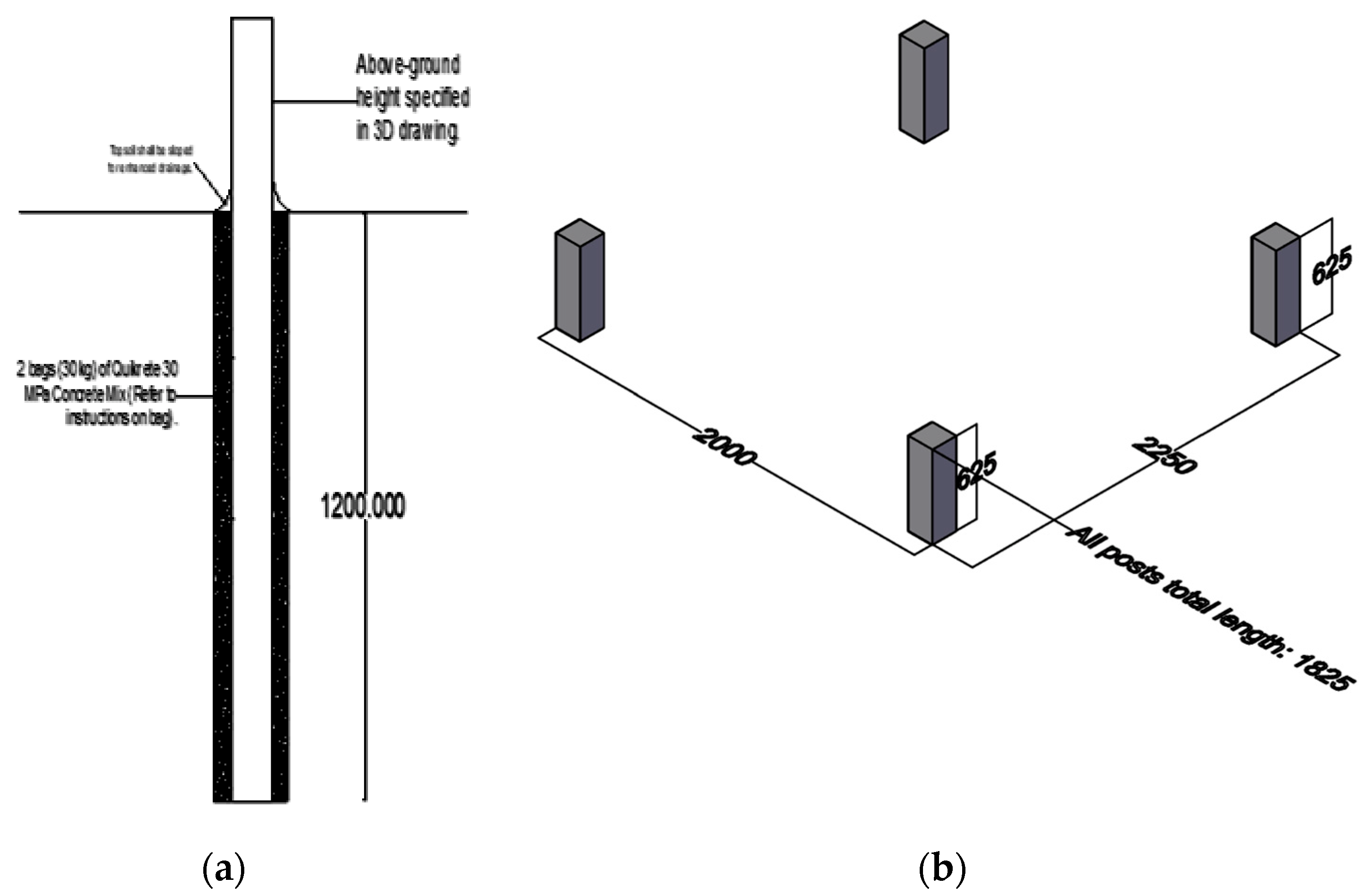
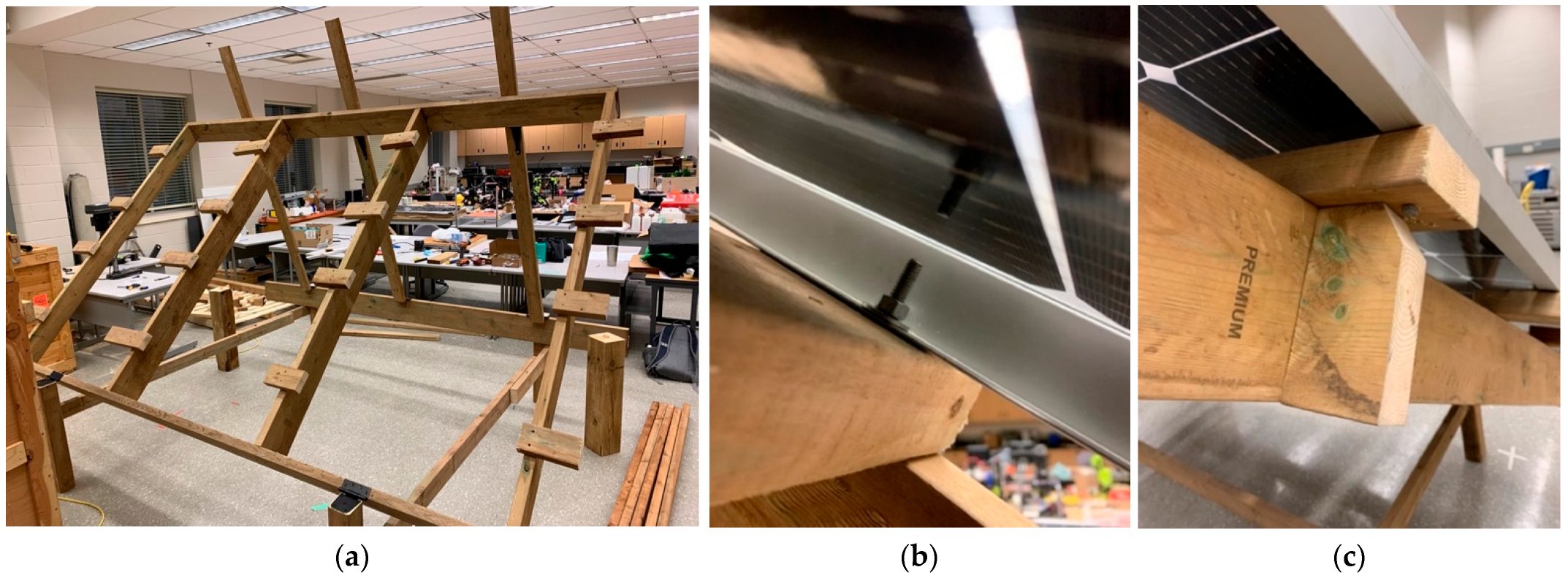
To begin, four holes at least 250 mm in diameter are dug at least 1.2 m into the ground, as shown in Figure 1a, to prevent frost heaving of any soil type, according to Table 9.12.2.2 in the National Building Code of Canada (NBCC) [40]. The 4 × 4 posts should have a center-to-center spacing, as described in Figure 1b, all cut to 1.825 m.
A 2 × 8 × 10 beam can then be installed onto the back posts, as shown in Figure 2. The overhang beyond each post is 0.5 m. The beam is to be installed to the posts with 3″ brown deck screws and one galvanized nut, bolt, and washer per post. If the posts are subject to ground movement, temporary 2 × 4 bracing can be installed to hold the system up during construction, as shown below. These braces can then be removed once the footings are stiff and secure.
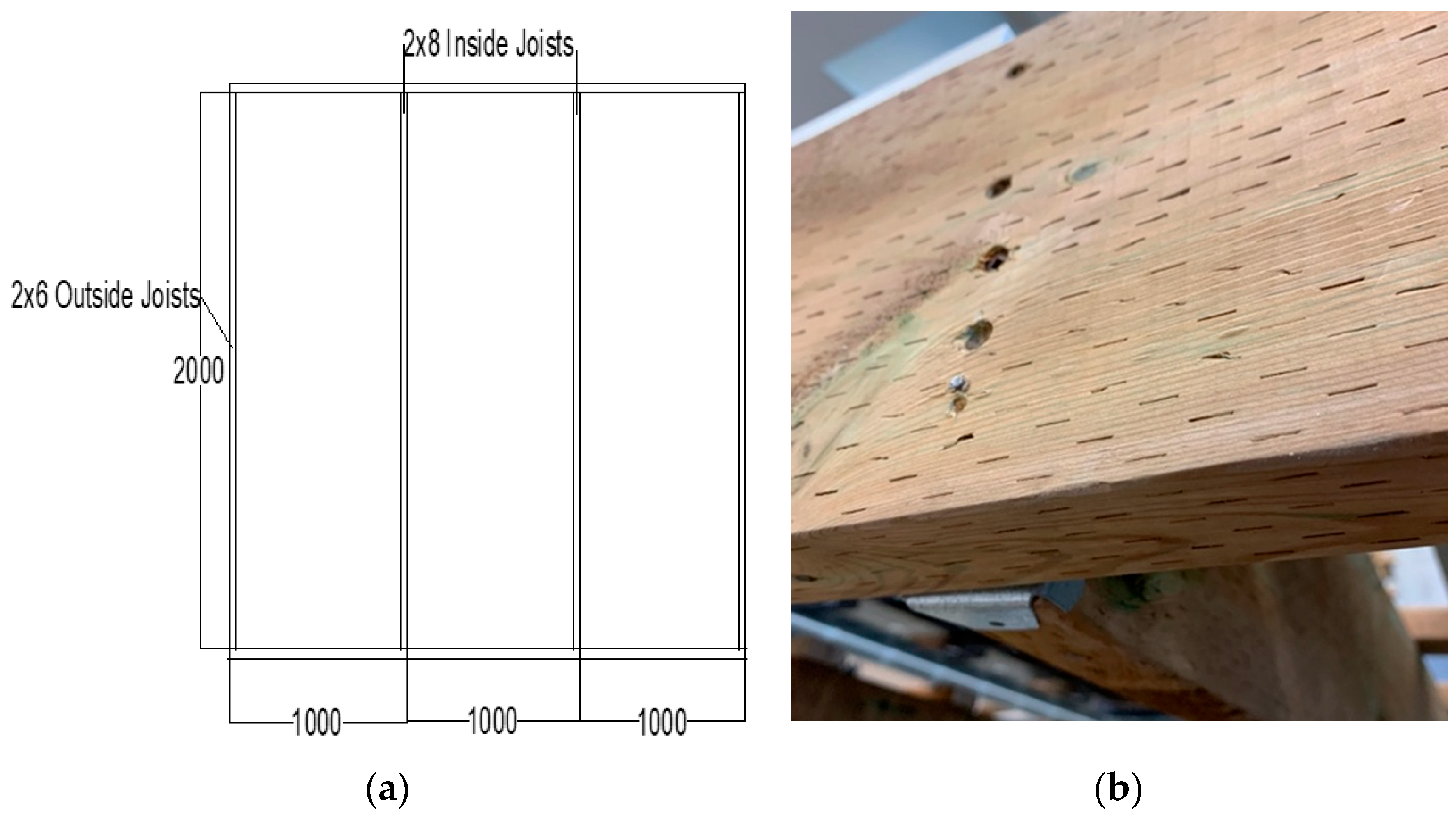
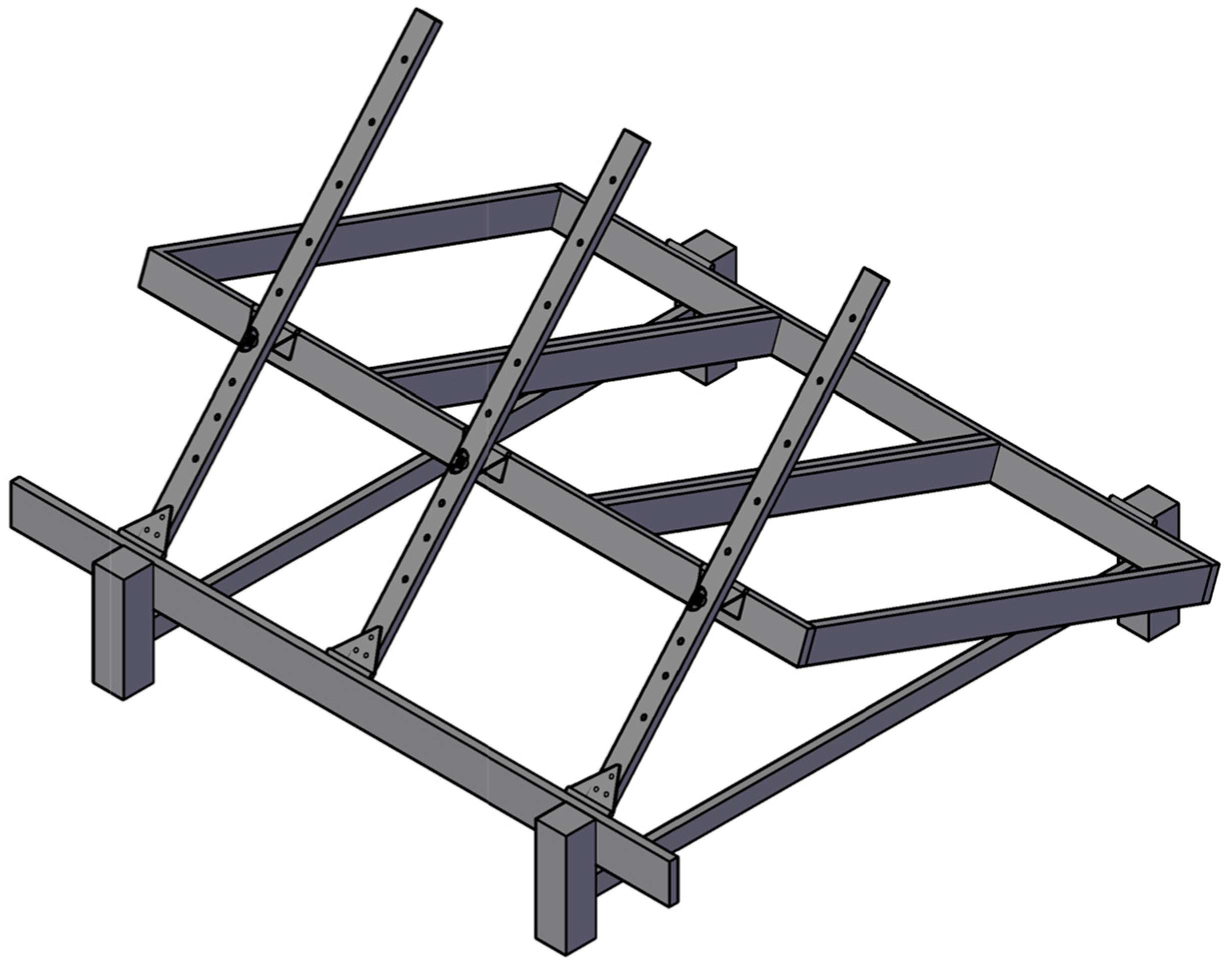
Once the base is installed, the frame can then be assembled, as shown in Figure 3a, using 2 × 6 outside joists and 2 × 8 inside joists connected to 2 × 8 beams. Connections, as shown in Figure 3b, should be assembled using fence brackets and 1-1/2″ joist hanger nails. Additionally, 4 3″ brown deck screws per joist should be installed to further sink the joist into the beam and to improve load transfer between the members.
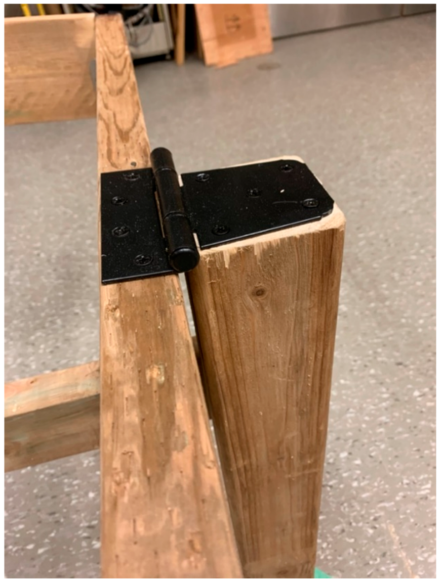
The frame can then be connected to the two front posts using 3-1/2″ traditional gate hinges. The 2 × 8 of the frame should be connected to the top of the post, as shown in Figure 4.
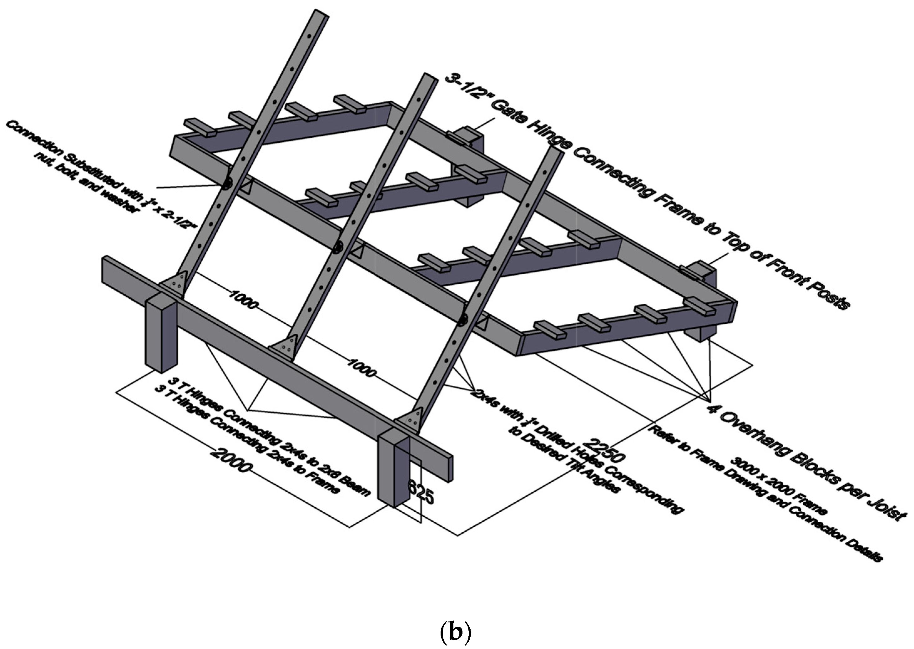
Three 2 × 4 s should then be cut to a length of 2 m. This will allow for a maximum tilt angle of 60 degrees. These 2 × 4 s will be used as the adjustable back supports for the system. Three galvanized gate T hinges will be connected between the joists on the frame, and another three will be connected on the beam, as shown in Figure 5.
Holes of 1/4″ should be drilled in the 2 × 4 s based on the desired tilt angle, as shown in Figure 6a. Align the frame hinges with the hole for the given tilt angle, and secure the connection with a 1/4″ nut, bolt, and washer, as shown in Figure 6b. While drilling the 2 × 4 s, temporary supports or extra helpers should be used to hold the frame up to prevent damage.
Once the joists are installed, scrap pieces of lumber can be cut into blocks and installed onto the joists with two screws, as shown in Figure 7a. These blocks serve as the connection between the module and the lumber and can be adjusted to match the holes of the module frame. The overhang of these blocks shall not exceed 100 mm. Once these blocks are installed, the modules can be placed onto the blocks. Drill a ¼″ hole through the block and insert a ¼″ × 2-1/2″ galvanized bolt from under the system. Then, place the module onto the bolt, and secure the connection with a nut and washer, as shown in Figure 7b. To enhance the load transfer to the joist, place another block under the overhanging block, and screw the second block into the joist, as shown in Figure 7c.
Once all connections are secured, the build is complete (Figure 8a). The system can then be disassembled in the reverse order it was initially constructed. Figure 8b provides a detailed back view to ensure all components of the system are present.
Annually, the bolt connections should be checked to ensure loose nuts are retightened. When possible, it is best practice to brush off snow from the modules to minimize creep in the lumber.
3.3. Build Time
The system requires at least two builders for installation. Refer to Table 3 for the typical time to complete each component per two builders.
To adjust the angle of the system, the nuts on the 2 × 4 s should be loosened, and the bolts should be taken off the hinges. It should be noted that once all the bolts are taken off, the system is free to fall and damage the racking frame. Approximately 150 lbs of force is required to keep the frame and modules from falling. Thus, temporary supports or extra help should be used to hold the frame up while repositioning the system to a new angle. Lift or drop the frame to the desired angle, then align the hinges with the drilled holes designated to that angle. The tilt angle can be found by using an angle level or by calculating the arctan of the frame’s rise divided by the run. Secure the connection with the nut, bolt, and washer. For higher angles, it can be difficult to lift the system, and thus, more help may be required. Refer to Table 4 for approximate adjustment times and recommended number of workers based on the desired tilt angle.
Following the calculations shown in Appendix A for the structural analysis, the forces and deflections of the system, specifically for the London, Ontario, system, have been summarized in Table 5. These values represent the worst-case scenario that governs the design of this system. When constructing a system, it is important to follow the structural design process in Appendix A to ensure the system can withstand the design load outlined in Appendix A. Depending on the design load, smaller members can be selected, and thus the net cost of the system can be reduced such that the maximum shear, moment, deflection, and axial forces are less than the capacities shown in Appendix A.
3.4. Energy Simulation Results
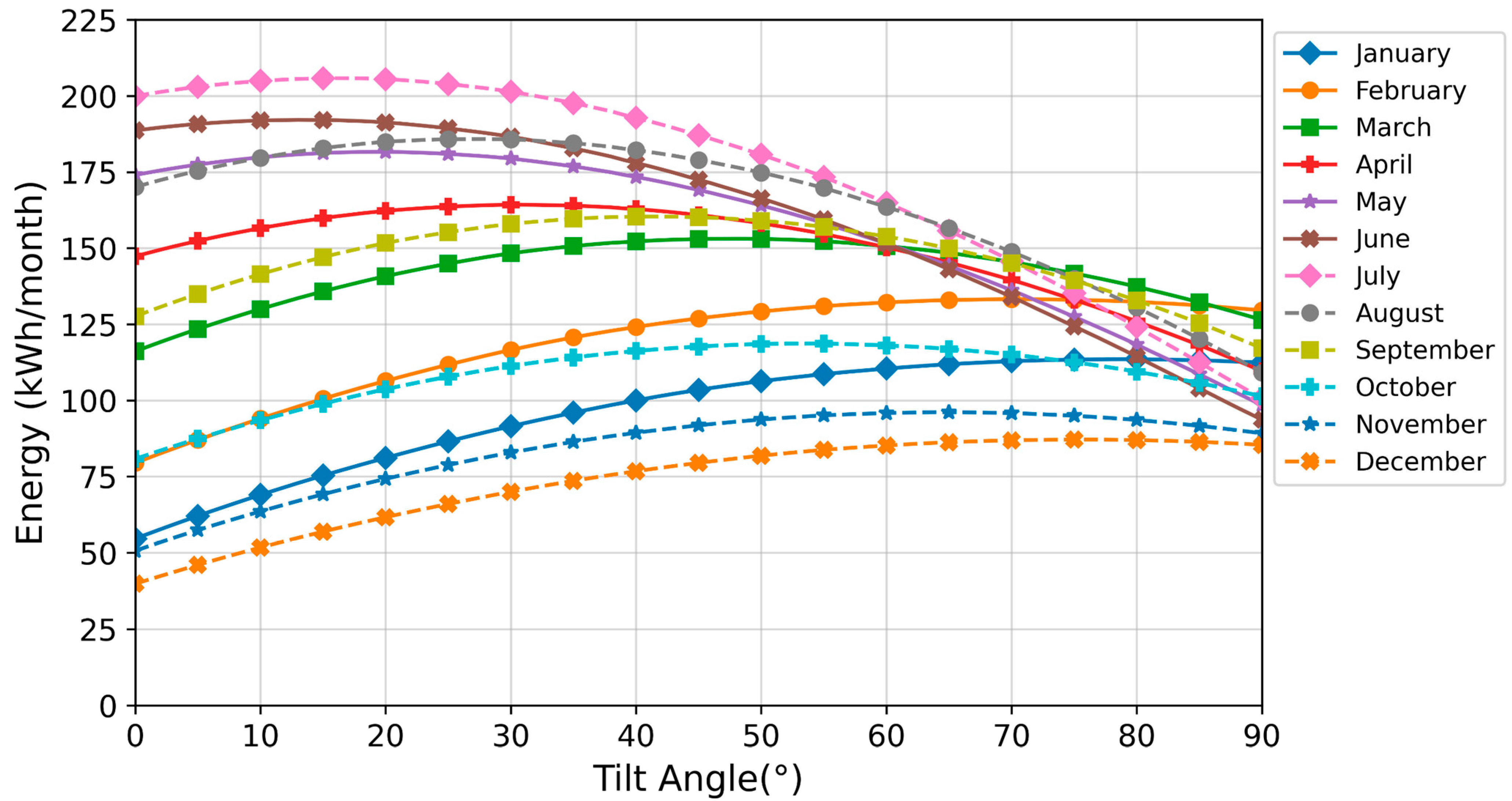
The results of the base model simulation are displayed in Figure 9, which shows the monthly energy production of the system during the first year for different tilt angles ranging from 0° (horizontal modules) to 90° (vertical modules) in steps of 1° for the city of London, ON, Canada.
The bell shapes of the monthly energy production curves show the value of the optimal angle for maximum energy generation each month. The monthly optima tilt angles are reported in Table 6. According to the values in Table 6, the system is at its highest tilt angle (79°) at the beginning of the year. The system has to be lowered every month until it reaches its lowest optimal tilt angle in July (16°) and has to be lifted again between August and January.
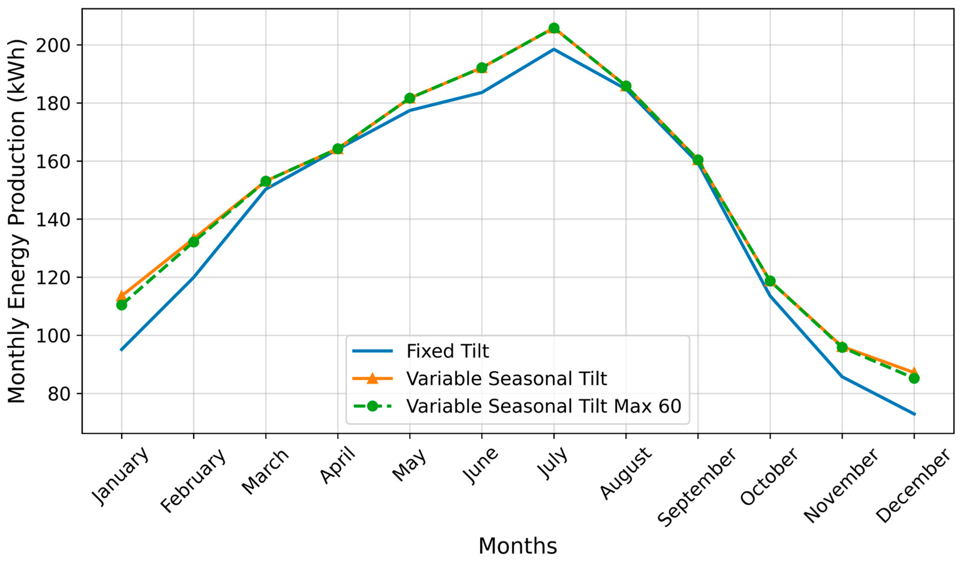
Three different energy simulation scenarios are analyzed. The first scenario results are shown in Table 6, the second scenario results cap the maximum adjustable tilt angle at 60°, and the third scenario fixes the optimal yearly tilt angle at 34°. The results of the simulations of the three scenarios are shown in Figure 10.
The results clearly show that the multi-tilt system produces more energy every month than the fixed-tilt as it uses seasonal tracking to optimize the solar energy harvested throughout the year. The maximum energy production gain of the optimum tilt angle system compared to the fixed-tilt racking system was 17% in December. Even in April, where the graph shows a similar energy production trend for the two systems, there is a small production gain from the multi-tilt of 0.13%. Furthermore, capping the maximum angle of the multi-tilt system to 60° only has a noticeable impact on the energy production of the system during January and December in the case of London, Ontario. During these months, the production is expected to be lower because of snow-related losses in Canada [41] and Ontario in particular [42,43], even if somewhat mitigated with bifacial PV modules [44]. Although, it should be pointed out that with the impacts of climate change, these losses are expected to decrease in the future [45].
3.5. Economic Analysis Results
The economic analysis of the system is shown in Table 7. As can be seen in Table 7, the open-source design provided in this study costs less than a third of the commercial equivalent variable tilt angle racking system.
The results in Table 7 show the lifetime energy production of the PV system, the racking cost, the LCOE of the racking, and the cost of each racking system per Watt. The racking systems (metal or wood) with an optimal variable seasonal tilt angle show the best lifetime energy production (42.15 MWh), which is 5.2% more energy generated by the fixed-tilt system (40.07 MWh). Even when the maximum angle of the wooden racking with variable tilt is limited to 60°, it generates 4.8% more energy (42.0 MWh) than the fixed-tilt system. In terms of LCOE, the wooden racking systems show similar LCOE (~CAD 0.01/kWh), and their LCOE represents only 29% of the LCOE of a commercial metal racking (CAD 0.033/kWh) serving the same purpose.
4. Discussion
4.1. Wooden Racking for Agrivoltaic and Impact of Labor Cost
The impact of the increase in energy production from the fixed-tilt wooden racking system to the variable angle wooden racking is seen in the LCOE of the two systems. Despite the wooden fixed-tilt system having a lower capital cost than the variable tilt wooden racking, they both have similar LCOE (~CAD 0.01/kWh). This is a crucial argument in determining which racking system to adopt. Specifically, the variable angle wooden racking design proposed in this study and the fixed-tilt wooden racking proposed by [36] are suitable for providing standalone clean solar PV energy to remote locations.
When the variable tilt wooden racking is compared to a commercial metal racking serving the same purpose (variable seasonal tilt angle) and purchased in Canada [46], the two systems have the same lifetime energy production. Nevertheless, the wooden racking is less costly than the commercial metal racking. In this study, data have been collected regarding the manpower and time needed for changing the angle of the proposed system seasonally (see Table 4). When the numbers in Table 4 are applied to the case of London, Ontario, the total annual labor time for changing the tilt of the wooden racking system is 1.9 person-hours/year, representing 47.5 person-hours during the lifetime of the wood racking system (25 years). Therefore, even when the labor cost for changing the tilt angle is factored into the wooden racking system’s cost, it remains economically more feasible than the commercial metal racking as long as the labor cost does not exceed CAD 21/hour. CAD 21/hour is 50% higher than CAD 14/hour, which is the average minimum wage across Canada [47]. Furthermore, this assumption is conservative as there is no information regarding the manpower required to change the tilt angle of the commercial metal racking. Hence, if the commercial metal racking requires more than one person to operate, the economic advantages of the variable tilt wooden racking system will be increased. On the other hand, when the labor cost is considered in the calculation of the variable angle wooden racking (as high as CAD 0.20), then the fixed-tilt wooden system is economically more viable. This does not, however, account for the additional benefits provided by the variable angle racking for specific applications such as agrivoltaics (see Section 4.2).
It should also be pointed out that there are several circumstances where the labor cost is effectively zero. For small-scale DIY systems [17], where prosumers are not charging themselves to vary the tilt angle of their own system or there is no opportunity cost to invest the few minutes once a month to change the tilt angle, the effective cost is zero, similar to businesses with salaried employees or even hourly employees where there is no cost to reassigning a few minutes once a month (e.g., secretaries manning a phone).
4.2. Agrivoltaics
Agrivoltaics in farmlands is a promising strategy for the co-development of land for both PV electrical generation and agriculture [48,49]. Services provided by agrivoltaics include: (i) renewable electricity generation, (ii) decreased greenhouse gas emissions, (iii) increased crop yield, (iv) plant protection from excess solar energy, (v) plant protection from inclement weather such as hail, (vi) water conservation, (vii) agricultural employment, (viii) local food, and (ix) increased revenue [50]. Benefits (i) and (ii) are well-established for all PV systems as they produce renewable electricity, which can offset greenhouse gas (GHG) emissions from fossil fuel-based electricity production [51]. From a farmer’s perspective, agrivoltaics also ensure that land remains productive during the winter by generating electricity year-round. Strikingly, agrivoltaics actually increase crop yield for a variety of crops [52,53,54,55,56], which along with solar electricity generation, substantially increases land-use efficiency [57]. Crops grow better with some PV-related shading because the PV array creates a microclimate beneath the modules that alters air temperature, relative humidity, wind speed, wind direction, and soil moisture [58]. Agrivoltaics also protects crops not only from excess solar energy preventing heat stress but also from inclement weather such as hail, while the PV performance can increase because of lower operating temperatures caused by the plants [54,59,60]. Combining PV and agriculture has the potential to increase global land productivity by 35–73% [61] while minimizing agricultural displacement for energy production [49,61,62]. Additionally, the microclimate created by agrivoltaics provides more efficient use of water and water conservation [63,64,65,66]. Furthermore, the novel variable tilt racking system analyzed here is particularly useful from an agrivoltaic perspective. The variable angle system will allow having the same LCOE as the fixed-tilt but will offer additional advantages specific to agrivoltaic farms, such as raising the modules to the selected highest angle to facilitate harvesting, planting, or weeding. In addition, the tilt angle can be lowered to protect the plants, for example, if a hail warning is issued. The labor involved with this tilt angle changing is trivial compared to that of farming, and additional farm labor is not always seen as a negative. By maintaining the land for use in agriculture, employment of farmers remains intact, and these farmers provide local sources of food along with all of the concomitant benefits [67,68]. Thus, agrivoltaics is looked at favorably not only by the PV community [69] but also by farmers [70] and farming communities [71]. The combination of farming and PV electricity generation increases revenue per acre for the farmer, and the local community also benefits from protecting access to fresh food and renewable energy [72]. Advanced inverter management can also provide stability [73] to rural electric grids and improve their power quality [74,75,76] if used in agrivoltaic systems. Finally, if the agrivoltaic system also includes storage, it can be used to create emergency islanded power grids that can reduce outage impacts [77,78], which may be particularly useful for isolated communities. For all these reasons, the system described here is perhaps best suited for small-scale agrivoltaics.
Lastly, the impact of the microenvironment for this type of racking system should be considered in the performance of the PV. Considerable work has been conducted to show that cooling PV modules with water by humidification by placing wet sacks at the back end of the PV module, water cooling by flowing the water on the front end of the module, and the combination of these two strategies improve performance in warm and humid climates [79]. Similarly, it is well-established that agrivoltaics create a microclimate under the PV modules that have similar but lesser PV performance benefits from direct intervention measures [80,81,82]. Although the wet sack method is not easily integrated into agrivoltaic wood-based racking systems because of compromising the agricultural potential, there is a potential for future work to consider the use of front-side cooling of agrivoltaic PV by integrating it into the irrigation of the crops (e.g., water is first used to cool the PV and then collected and dispersed to water the crops. Future work is needed to explore this potential both technically and economically.
4.3. System Location Sensitivity
The energy production of the system is simulated for different locations in the northern hemisphere to assess and compare the energy production performance of the fixed-tilt wooden racking proposed by Vandewetering et al. [36] and the variable tilt wooden racking proposed in this study. The location considered for the simulation and the latitude of those locations are shown in Table 8.
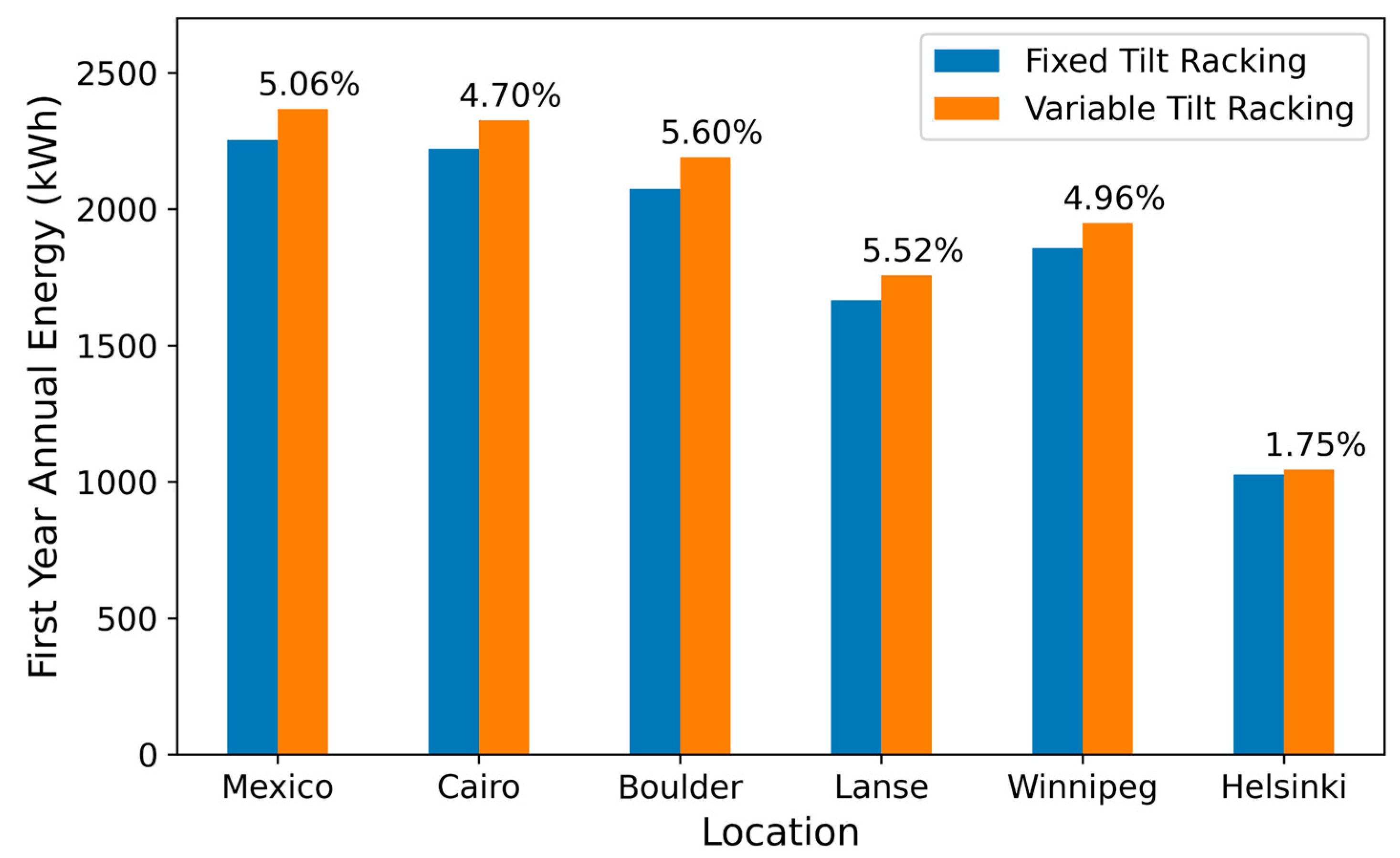
Figure 11 shows the comparison of the annual energy production during the first operational year for the locations shown in Table 8. The results in Figure 11 show clearly that wherever the two systems are located, the variable tilt system will produce more energy than the fixed-tilt racking for the same operational conditions. Nevertheless, it is necessary to mention that the actual LCOE of the two systems is highly dependent on the local wood prices. This sensitivity is briefly discussed in Section 4.4, and a more detailed wood price sensitivity analysis is available in previous work [36].
4.4. Wood Price Sensitivity
The system is highly sensitive to the price of lumber, which has shown to be volatile in the sensitivity analysis in the design in [36].
The costs of this design will also be dependent on the local sources of wood being available and, if imported, the taxes and import duties. Refer to Table 9 for the typical price of a construction grade pressure-treated 2 × 4 × 8 in various countries.
This open-source wood PV rack is (1) made from locally accessible, sustainable, renewable materials, (2) can be fabricated using simple hand tools by the average consumer, (3) has a 25-year lifetime to be equivalent to common PV warranties, (4) is structurally sound in order to weather high wind speeds and major snow loads (depending on the region), (5) has a low cost and (6) that is shared using an open-source license so that many people can fabricate it themselves, or companies can make versions to offer in their local markets.
4.5. Limitations
This system is entirely built with materials available at local hardware stores and requires a few hours of labor to complete the build. Since the multi-tilt system is not pre-assembled, this system is mainly targeted toward do-it-yourselfers (DIYers). The limitation to DIY multi-tilt racking is that many people, such as the elderly or physically disabled, may have to hire a general contractor to build the system, which adds a labor cost to the system build. Depending on the location and labor rates, this would diminish the economic advantages shown here. Nevertheless, metal racking systems also require initial labor costs if not built by the owner, thus making the cost comparison between wood and metal racking still valid.
The primary benefit of this design is to convert physical labor into electrical power, but on a three-panel array, the difference in power remains small. By making many replications of this three-panel array, the benefit can be scaled up to produce significantly more power for the owner. Table 10 summarizes the amount of extra energy generated in a lifetime from monthly tilt adjustments in many scenarios, where this system is scaled up to satisfy the energy demand of practical applications. By scaling up the number of three-panel arrays, both the generated power and economic benefit of monthly adjustments proportionally scale up. It should be noted that costs can further be reduced in scaled-up systems since many hardware stores honor a contractor discount to those who purchase orders in bulk. This makes all economic estimates used in this study extremely conservative for any form of scale up case.
Despite the technical and economic benefits the multi-tilt system provides, it is more difficult to install compared to fixed-tilt systems. Not only does it require more time to install, but it is also more labor-intensive, especially when measuring and drilling holes into the 2 × 4 s while holding the large frame in place. To mitigate this, extra lumber to serve as temporary bracing and support can be used to hold the frame and posts up while measurements and cuts are being made.
For agrivoltaic applications, the use of pressure-treated lumber can pose the threat of introducing toxic chemicals into the vegetation. Since the 1930s, pressure-treated lumber contained chromated copper arsenate to protect the wood from rotting, which caused major health and environmental concerns but has been discontinued and replaced with copper azole preservative since 2004 [85]. Copper azole is a much safer alternative since it removes exposure from chromium and arsenic, and copper is already abundant in soil and groundwater, but high doses of copper can result in severe liver and kidney damage [86]. Therefore, if this system is in close contact with vegetation, it is highly advised to prevent pressure-treated lumber from contacting the soil. Natural alternatives such as cedar lumber can be used, but the cost is at least 2.5 times that of pressure-treated. The best solution to eliminate soil contact is to extend the concrete footing up and above the ground. This may require using an extra bag of concrete in each footing to ensure enough mix reaches a significant level above the ground. Future work in sand and acrylonitrile styrene acrylate waste composites [87] or other plastic composites may serve as a less permeable alternative to concrete footings to further prevent soil contamination in some applications.
5. Conclusions
This study detailed the designs of a novel variable tilt angle open-source wood-based PV racking system. The system costs less than one-third of the CAPEX of variable tilt angle commercial racking solutions. These lower costs make it economical in some contexts for labor to be exchanged profitably for higher solar electric output. The results of this study show that the racking systems with an optimal variable seasonal tilt angle present the best lifetime energy production, with 5.2% more energy generated compared to the fixed-tilt system (or 4.8% more energy, if limited to a maximum tilt angle of 60°). Thus, a few minutes of labor per kW can be traded for about 5% more annual solar electricity production. Both fixed and variable wooden racking systems show similar LCOE of less than 1 cent, which is only 29% of the LCOE of commercial metal racking. The economic analysis found that in several contexts, the novel variable tilt rack provides the lowest cost option even when modest labor costs are included. Finally, the novel variable tilt racking design shown here has several specific advantages over fixed-tilt designs for applications such as agrivoltaics.
Author Contributions
Conceptualization, J.M.P.; methodology, N.V., K.S.H.; software, K.S.H.; validation, N.V., K.S.H.; formal analysis, J.M.P., N.V., K.S.H.; investigation, N.V., K.S.H.; resources, J.M.P.; data curation, N.V., K.S.H.; writing—original draft preparation J.M.P., N.V., K.S.H.; writing—review and editing, J.M.P., N.V., K.S.H.; visualization, N.V., K.S.H.; supervision, J.M.P.; funding acquisition, J.M.P. All authors have read and agreed to the published version of the manuscript.
Funding
This research was funded by the Thompson Endowment and the Natural Sciences and Engineering Research Council of Canada (NSERC).
Institutional Review Board Statement
Not applicable.
Informed Consent Statement
Not applicable.
Data Availability Statement
Data will be made available upon request.
Acknowledgments
The authors would like to thank Paul Vandewetering of Paul’s Build-All for assistance in the construction of the variable angle rack.
Conflicts of Interest
The authors declare no conflict of interest. The funders had no role in the design of the study; in the collection, analyses, or interpretation of data; in the writing of the manuscript, or in the decision to publish the results.
Appendix A. Variable Tilt System Structural Analysis
It can be difficult to determine the specified design load for this system because the design load is dependent on the tilt angle, which will vary throughout the system’s life cycle. For the purpose of analysis, the angle that produces the heaviest combined wind and snow loads is any angle between 30 and 45 degrees, as suggested by the NBCC wind and snow design load procedure [40]. For London, Ontario, design loads of 1.80 and −0.81 kPa are yielded when following the procedure outlined in the design in [36]. To ensure that the system will not unexpectedly fail, the applied shear forces, bending moments, and deflections shall not exceed the limits of each structural member outlined in the National Design Specification for Wood Construction [88].
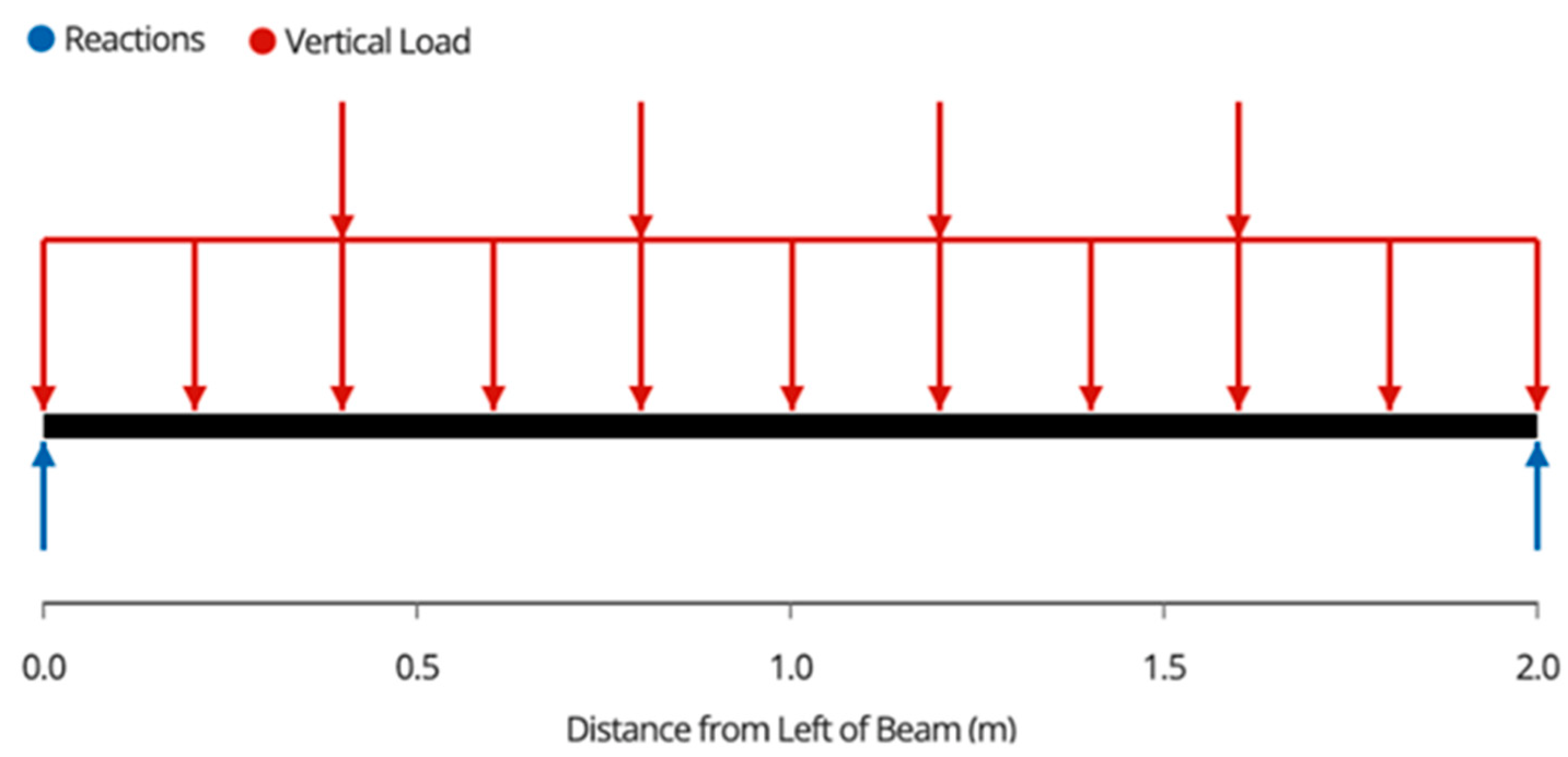
The net load is distributed evenly throughout the surface of the modules. As per the supplier of the modules [89], it is assumed that the panels have sufficient capacity to carry these loads. The load is then transferred from the panels to the joists. Each joist carries its own weight as a uniform distributed load, w, and four-point loads that represent the block connections. w is calculated using Equation (A1),
OW represents the own weight of the member, which needs to be multiplied by a factor of 1.25 because it is a dead load [90]. Since the required dimensions of lumber to carry the load is unknown, an assumption needs to be made (for example, assume 2 × 8) to carry out the analysis. If the assumption results in the maximum applied value being greater than the resistance values, then a larger member needs to be used.
The point loads can be calculated by dividing each joist’s tributary loading into four points because it is assumed that the load is distributed evenly throughout the modules. The tributary area represents how much width of the panels each joist is responsible for carrying. For example, in this three-module system, which is 3 m wide, the middle joists have a tributary width of 1 m (0.5 m on each side), and the end joists have a tributary width of 0.5 m (only one side). The value for each point load on the joists is calculated using Equation (A2),
Once w and the point loads are calculated, the free body diagram shown in Figure A1 for each joist can be made.
Figure A1.
Free body diagram of joists. Note that the two outside joists will have half the tributary area of the inside joists and thus will carry approximately half of the load.
Figure A1.
Free body diagram of joists. Note that the two outside joists will have half the tributary area of the inside joists and thus will carry approximately half of the load.

Each joist is supported a beam on each end. The reaction and thus the load that each joist transfers to each beam is calculated using Equation (A3),
The shear force diagram throughout each joist is seen in Figure A2.
Figure A2.
Joist shear force diagram.

The maximum shear force occurs at the supports, and thus, the maximum shear is calculated as the reaction shown above.
The bending moment diagram in each joist is seen in Figure A3.
Figure A3.
Joist bending moment diagram.

The maximum bending moment of the joists occurs at the midspan. The maximum bending moment can easily be calculated using Equation (A4),
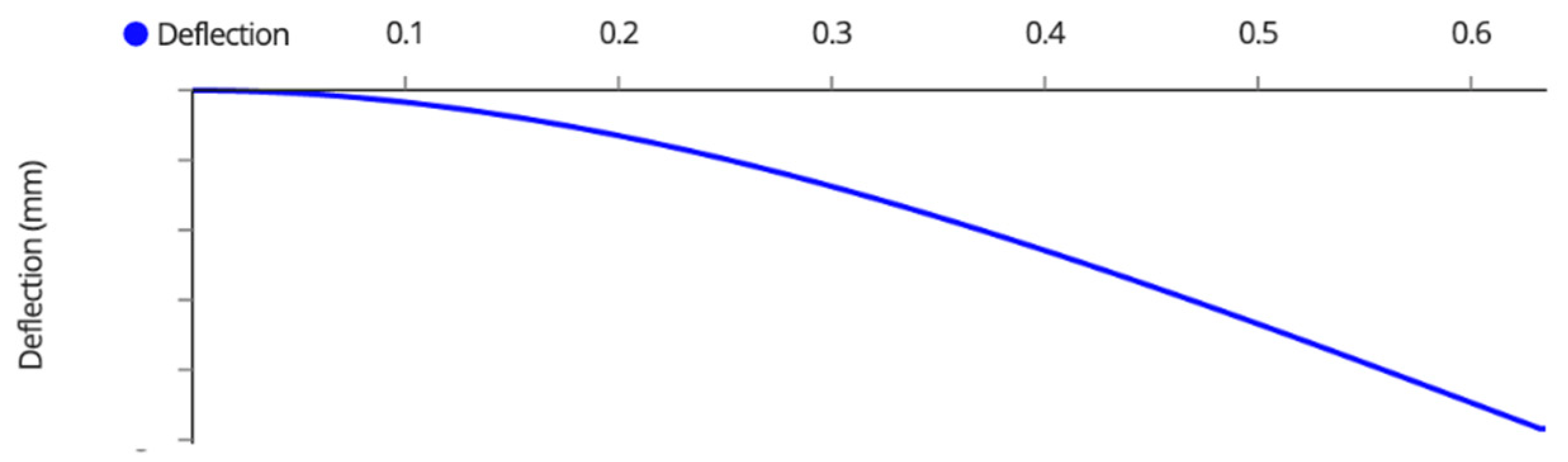
The deflection diagram throughout each joist is plotted in Figure A4.
Figure A4.
Joist deflection diagram.

The maximum deflection of the joists occurs at the midspan. For simplicity of analysis, assume the four-point loads serve as a uniform distributed load, and calculate the maximum deflection using Equation (A5),
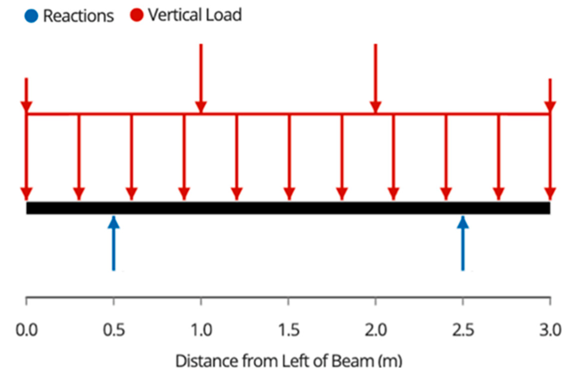
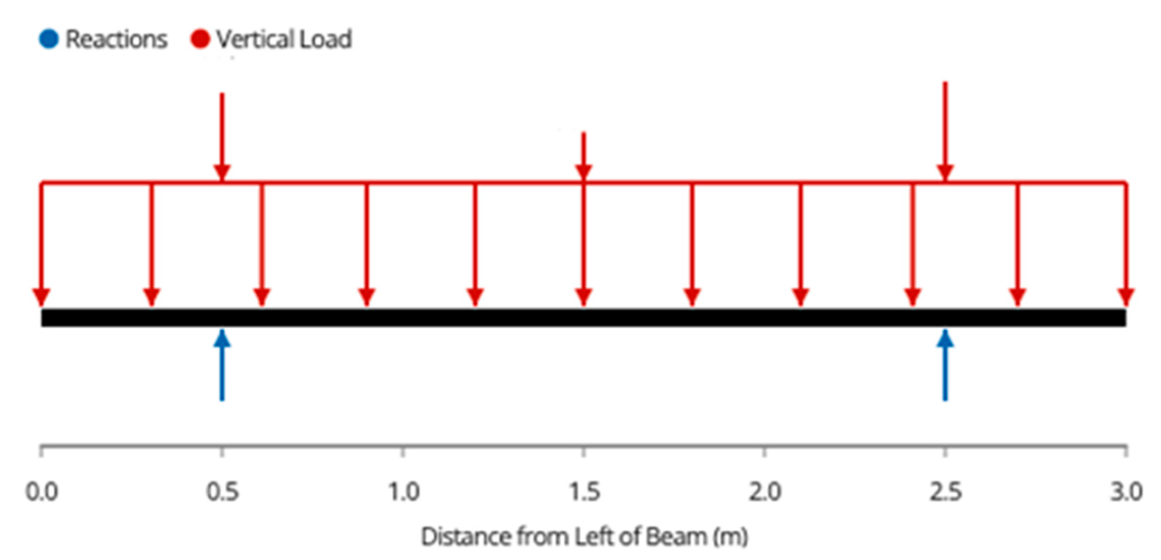
In the frame, half of the load will be transferred to the front 2 × 8, and the other half to the back 2 × 8. The free body diagram for the front 2 × 8 is shown in Figure A5.
Figure A5.
Beam free body diagram.

Due to the symmetric loading of the beams, the post loads or the support reactions are described in Equation (A6),
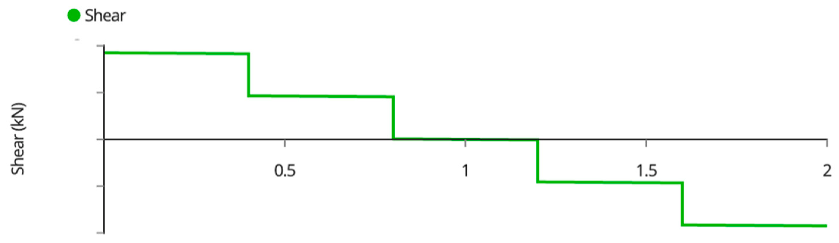
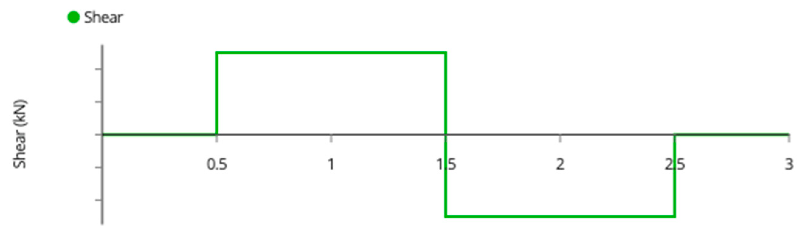
The shear force diagram for the beams is described in Figure A6.
Figure A6.
Beam shear force diagram.

The maximum shear forces occur on the inside of the reactions and are calculated using Equation (A7)
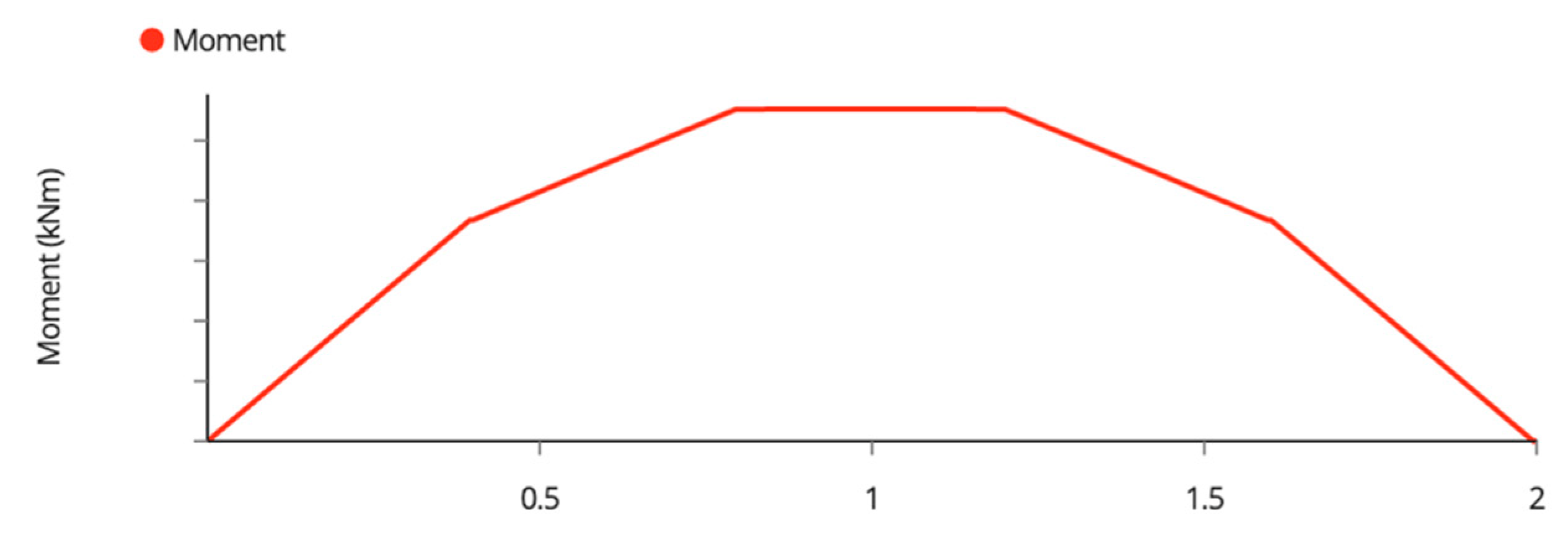
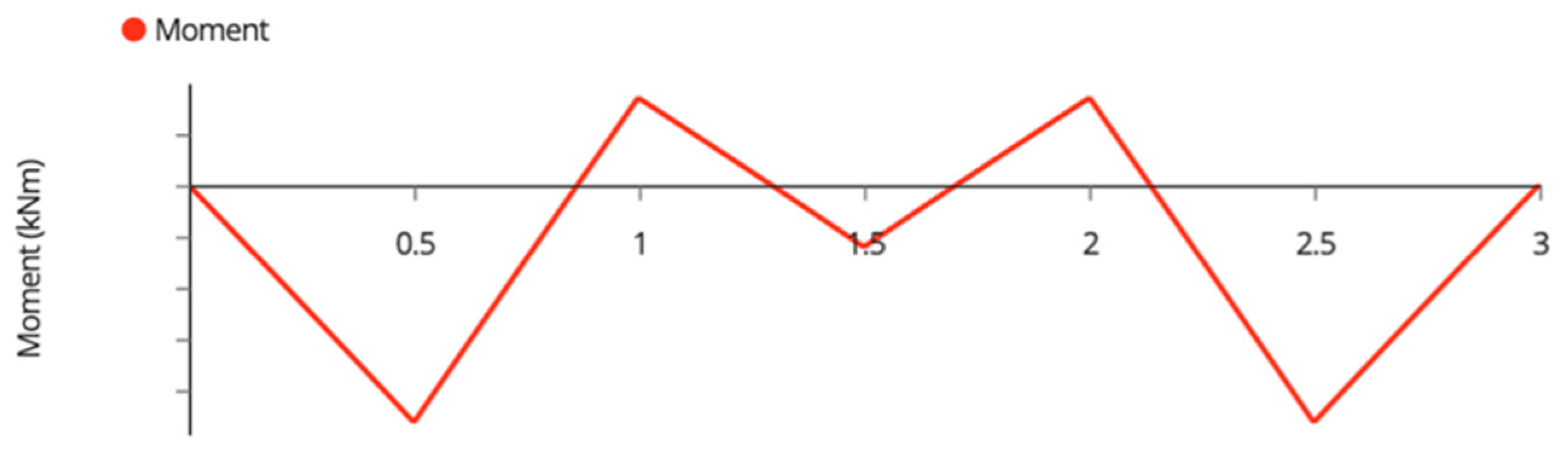
The bending moment diagram for the beam is shown in Figure A7.
Figure A7.
Beam bending moment diagram.

The maximum moment occurs at the supports and can be found by integrating the shear force throughout the first sixth of the beam, as described in Equation (A8) or by simply finding the area under the shear force diagram.
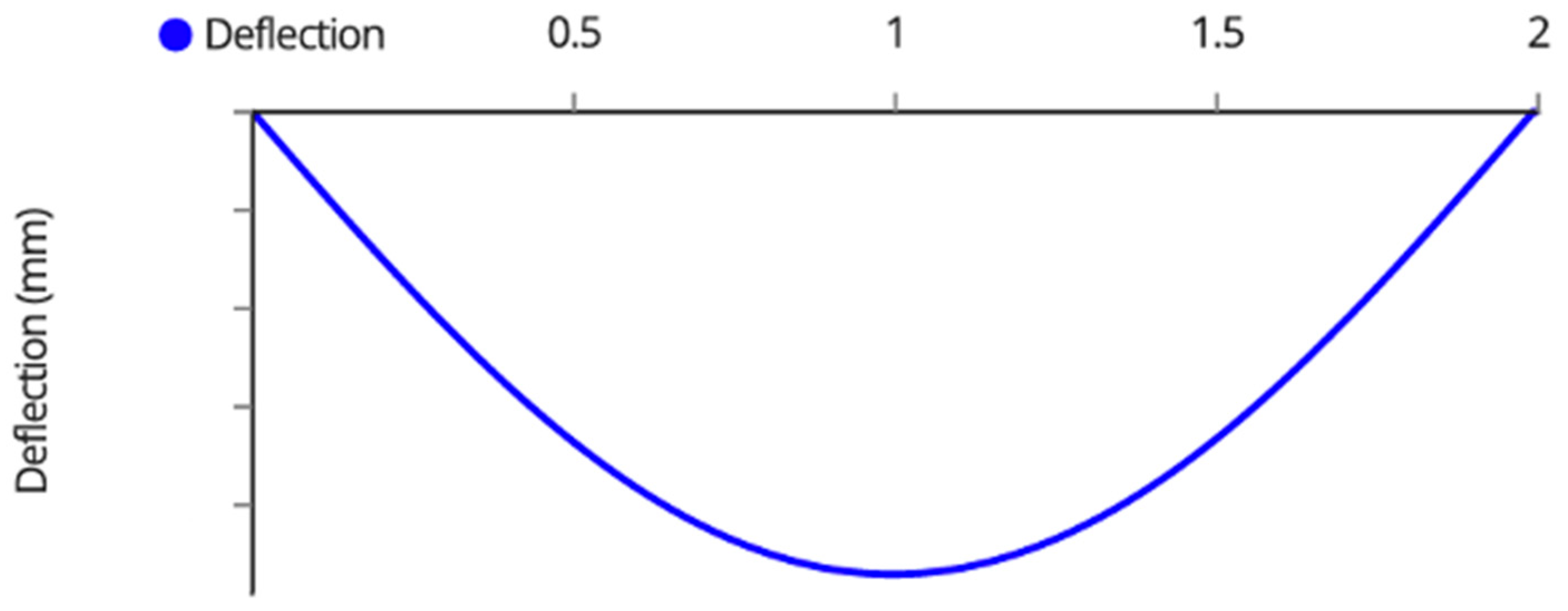
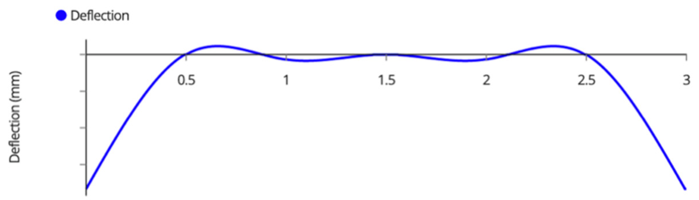
The deflection diagram is shown in Figure A8.
Figure A8.
Beam deflection diagram.

The maximum deflection occurs at the midspan and can be solved using the differential Equation (A9) and initial conditions below or by using the moment area theorem or virtual work method described in many structural engineering textbooks.
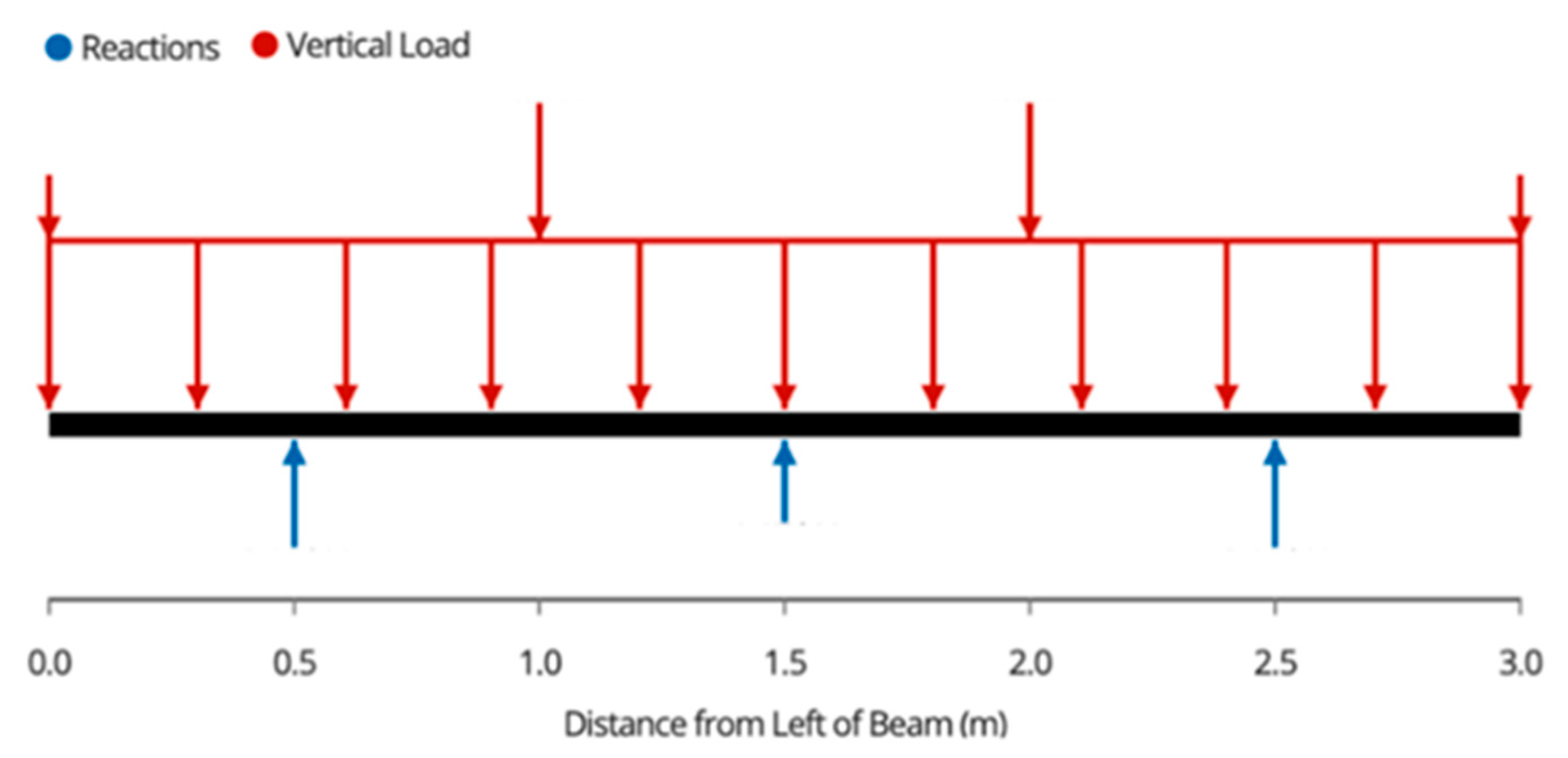
The back 2 × 8 in the frame is then supported by three hinges. The free body diagram for the beam is shown in Figure A9. This is an indeterminate structure, meaning that it has too many supports to be solved with static analysis and thus cannot be expressed with generalized equations. The structure can be solved by using finite element analysis or by an analytical method such as the moment distribution or slope-deflection method.
Figure A9.
Beam free body diagram for variable angle rack.

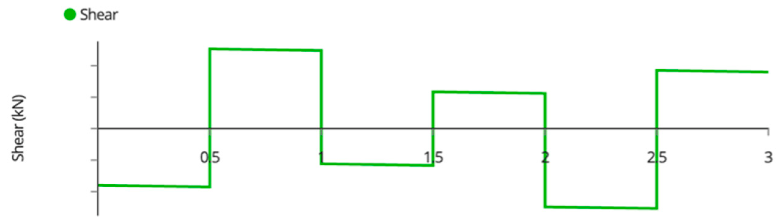
The shear force diagram for each beam is shown in Figure A10.
Figure A10.
Beam shear force diagram.

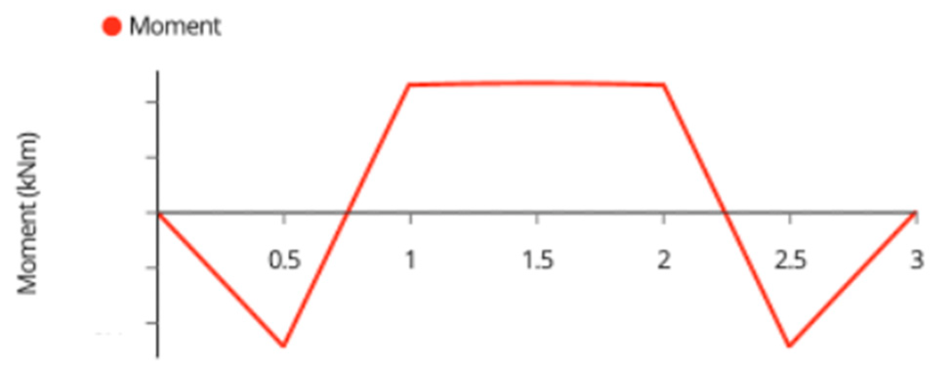
The bending moment diagram for each beam is shown in Figure A11.
Figure A11.
Beam bending moment diagram.

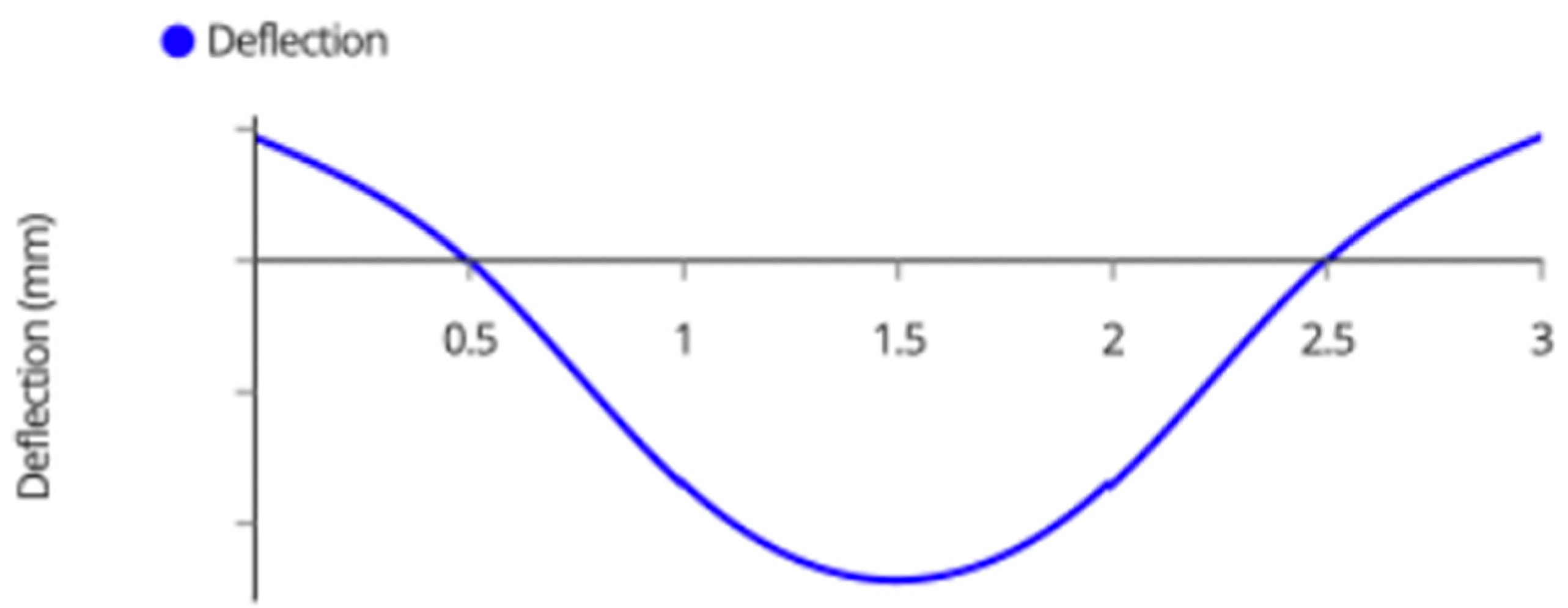
The deflection diagram for each beam is shown in Figure A12.
Figure A12.
Beam deflection diagram.

The load is then transferred to the supporting 2 × 4 via the T hinges. Since these hinges are free to rotate, the 2 × 4 s can be idealized as truss members in pure compression (the moments are released). The compressive force is equal to the reaction supporting the beam. These back supports are slender and thus should be checked for buckling using Equations (A10) and (A11).
After confirming that both Cbuckling and Cmax are less than Cr, the load can then be transferred to the bottom beam with the free body diagram shown in Figure A13.
Figure A13.
Bottom beam free force diagram.

The shear force diagram is shown in Figure A14.
Figure A14.
Bottom beam shear force diagram.

The bending moment diagram is shown in Figure A15.
Figure A15.
Bottom beam bending force diagram.

The deflection diagram is shown in Figure A16.
Figure A16.
Bottom beam deflection diagram.

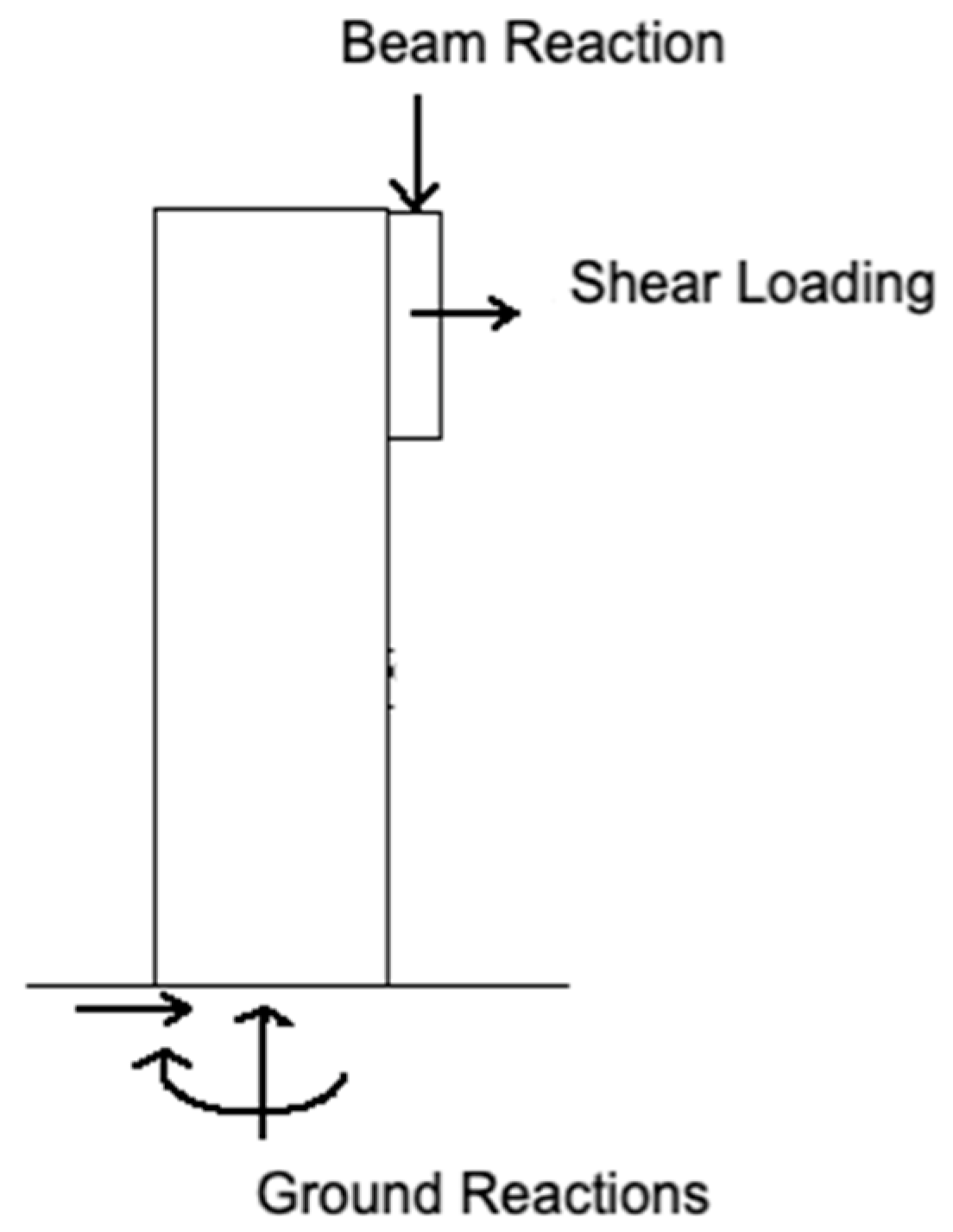
The load is then transferred to the posts. It should be noted that the posts are not loaded purely in compression; an eccentricity, e, described in the free body diagram in Figure A17, induces a bending moment.
Figure A17.
Post free body diagram.

The compressive load of the column is equal to the beam reaction solved above. Along with this compressive load comes a shear loading that is induced by wind and snow loads. This loading can act in either the left or right direction, but the load should be analyzed in the direction that induces bending in the same direction as the beam reaction. The magnitude of this shear load in each post is described in Equation (A12),
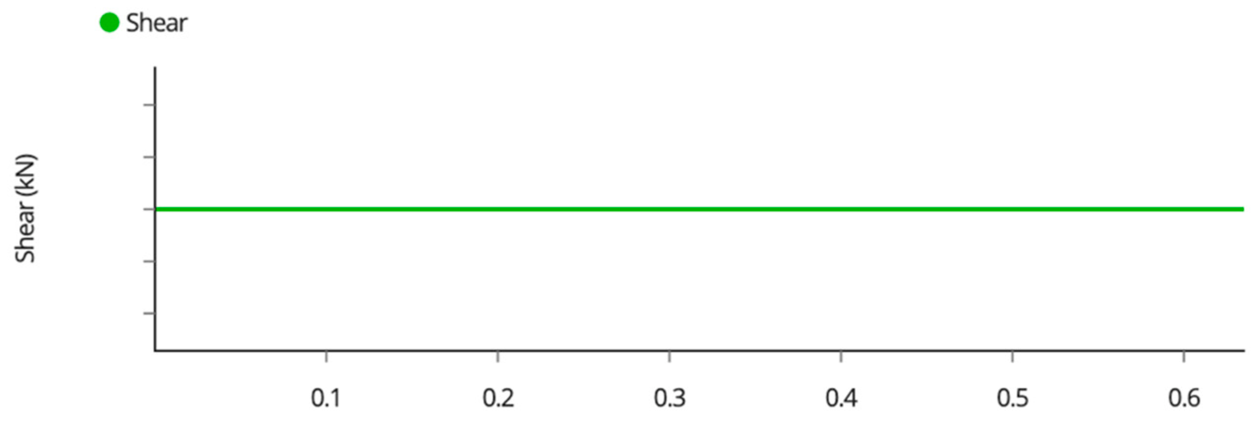
where θ is the tilt angle of the system. For conservative analysis, assume the lowest tilt angle of 0 degrees to maximize this load calculation. The post will serve as a determinant beam column. The shear force diagram is shown in Figure A18.
Figure A18.
Post shear force diagram.

The maximum shear can be calculated using Equation (A13),
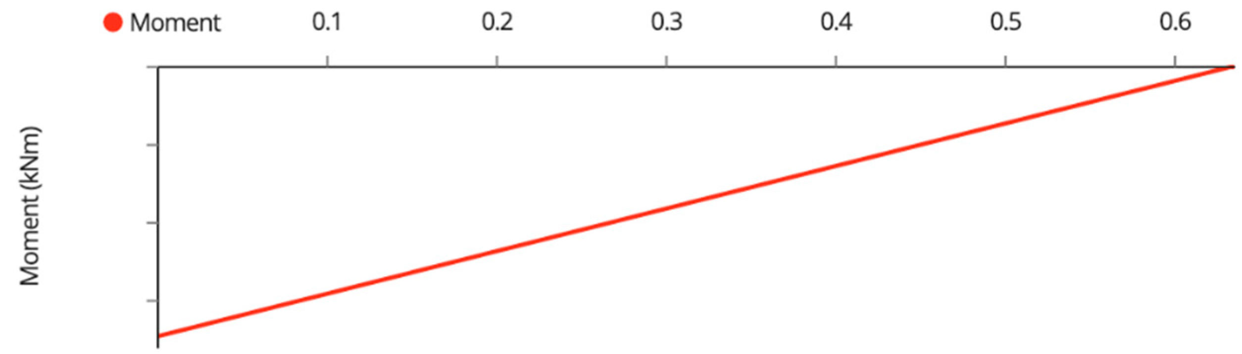
The bending moment diagram can be found in Figure A19.
Figure A19.
Post bending moment diagram.

The maximum bending moment can be calculated using Equation (A14).
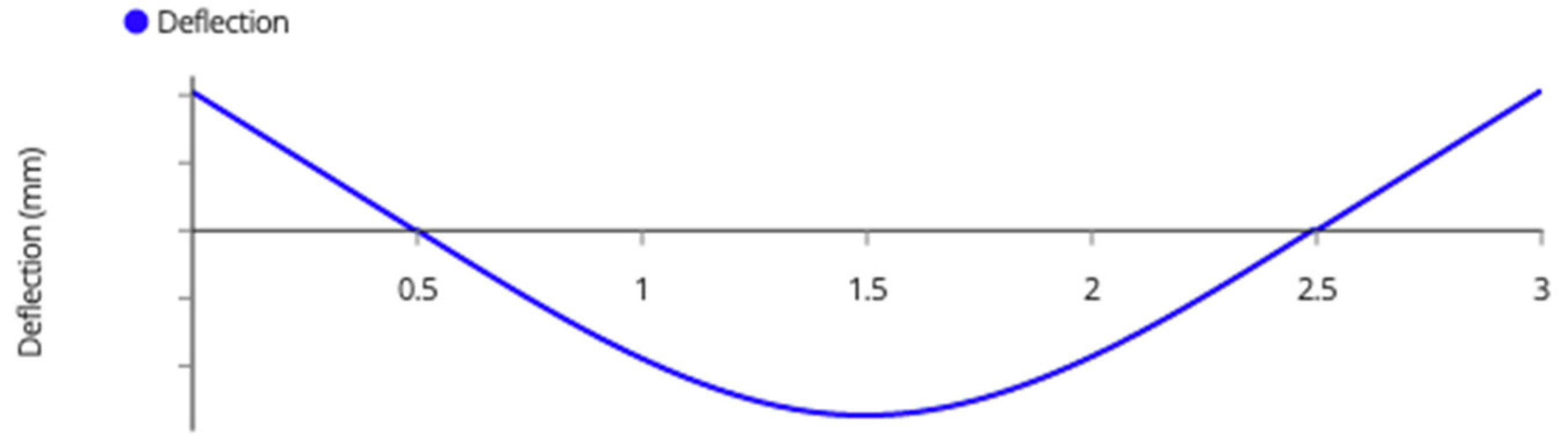
The deflection diagram is shown in Figure A20.
Figure A20.
Post bending moment diagram.

The maximum deflection can be calculated using Equation (A15).
Once all components of the post have been analyzed, the load will finally transfer itself to the ground. Table 9.4.4.1 of the NBCC provides maximum allowable bearing pressures for different types of soil and rock. In the worst case, soft clays support a maximum bearing pressure of 75 kPa [40]. To ensure, that the ground is not overloaded and settles, the bearing pressure can be calculated with Equation (A16),
If the applied pressure is more than the allowable, 150 mm of compacted clear stone gravel can be added to the bottom of the footing, or the footing diameter can be increased.
Throughout the system, each connection transfers the load from one member to another via a shear force within the fasteners that compose that connection. For bolts complying with ASTM A307A, the shear resistance of a ½″ carriage bolt holding the beams is about 23.8 kN, and the shear resistance of a ¼″ carriage bolt holding the modules is 5.21 kN [91], both of which are beyond the demand of these systems, and thus will not be critical to the design.
References
- Pearce, J.M. Photovoltaics—A path to sustainable futures. Futures 2002, 34, 663–674. [Google Scholar] [CrossRef]
- Fu, R.; Feldman, D.J.; Margolis, R.M. US Solar Photovoltaic System Cost Benchmark: Q1 2018; No. NREL/TP-6A20-72399; National Renewable Energy Lab.: Golden, CO, USA, 2018. [Google Scholar]
- How Much Do Solar Panels Cost? 2022 Guide. Available online: https://news.energysage.com/how-much-does-the-average-solar-panel-installation-cost-in-the-u-s/ (accessed on 10 May 2022).
- Branker, K.; Pathak, M.J.M.; Pearce, J.M. A review of solar photovoltaic levelized cost of electricity. Renew. Sustain. Energy Rev. 2011, 15, 4470–4482. [Google Scholar] [CrossRef] [Green Version]
- Dudley, D. Renewable Energy Will Be Consistently Cheaper Than Fossil Fuels by 2020, Report Claims [WWW Document]. Forbes. 2019. Available online: https://www.forbes.com/sites/dominicdudley/2018/01/13/renewable-energy-cost-effective-fossil-fuels-2020/ (accessed on 13 April 2020).
- Solar Industry Research Data. Available online: https://www.seia.org/solar-industry-research-data (accessed on 13 April 2020).
- Vaughan, A. Time to shine: Solar power is fastest-growing source of new energy. The Guardian, 6 October 2017. [Google Scholar]
- Barbose, G.L.; Darghouth, N.R.; LaCommare, K.H.; Millstein, D.; Rand, J. Tracking the Sun: Installed Price Trends for Distributed Photovoltaic Systems in the United States-2018; Berkeley Lab: Berkely, CA, USA, 2018. [Google Scholar]
- IEA. Solar PV—Renewables 2020—Analysis. Available online: https://www.iea.org/reports/renewables-2020/solar-pv (accessed on 7 April 2022).
- Levin, T.; Thomas, V.M. Can developing countries leapfrog the centralized electrification paradigm? Energy Sustain. Dev. 2016, 31, 97–107. [Google Scholar] [CrossRef] [Green Version]
- Lang, T.; Ammann, D.; Girod, B. Profitability in absence of subsidies: A techno-economic analysis of rooftop photovoltaic self-consumption in residential and commercial buildings. Renew. Energy 2016, 87, 77–87. [Google Scholar] [CrossRef]
- Hayibo, K.S.; Pearce, J.M. A Review of the Value of Solar Methodology with a Case Study of the U.S. VOS. Renew. Sustain. Energy Rev. 2021, 137, 110599. [Google Scholar] [CrossRef]
- Agenbroad, J.; Carlin, K.; Ernst, K.; Doig, S. Minigrids in the Money: Six Ways to Reduce Minigrid Costs by 60% for Rural Electrification. Rocky Mountain Institute. 2018. Available online: https://rmi.org/insight/minigrids-money/ (accessed on 28 February 2022).
- Alafita, T.; Pearce, J.M. Securitization of residential solar photovoltaic assets: Costs, risks and uncertainty. Energy Policy 2014, 67, 488–498. [Google Scholar] [CrossRef] [Green Version]
- Renewables International. Photovoltaics after Grid Parity Plug-and-Play PV: The Controversy 2013. Renewables. 2013. Available online: http://www.renewablesinternational.net/plug-and-play-pv-the-controversy/150/452/72715/ (accessed on 18 December 2015).
- Mundada, A.S.; Nilsiam, Y.; Pearce, J.M. A review of technical requirements for plug-and-play solar photovoltaic microinverter systems in the United States. Solar Energy 2016, 135, 455–470. [Google Scholar] [CrossRef]
- Grafman, L.; Pearce, J.M. To Catch the Sun; Humboldt State University Press: Arcata, CA, USA, 2021; ISBN 978-1-947112-62-9. [Google Scholar]
- Barbose, G.; Darghouth, N.; Millstein, D.; Cates, S.; DiSanti, N.; Widiss, R. Tracking the Sun IX: The Installed Price of Residential and Non-Residential Photovoltaic Systems in the United States; Lawrence Berkeley National Lab. (LBNL): Berkeley, CA, USA, 2016. Available online: https://www.osti.gov/servlets/purl/1345194 (accessed on 10 May 2022).
- Khan, M.T.A.; Norris, G.; Chattopadhyay, R.; Husain, I.; Bhattacharya, S. Autoinspection and Permitting with a PV Utility Interface (PUI) for Residential Plug-and-Play Solar Photovoltaic Unit. IEEE Trans. Ind. Appl. 2017, 53, 1337–1346. [Google Scholar] [CrossRef]
- Khan, M.T.A.; Husain, I.; Lubkeman, D. Power electronic components and system installation for plug-and-play residential solar PV. In Proceedings of the 2014 IEEE Energy Conversion Congress and Exposition (ECCE), Pittsburgh, PA, USA, 14–18 September 2014; pp. 3272–3278. [Google Scholar]
- Lundstrom, B.R. Plug and Play Solar Power: Simplifying the Integration of Solar Energy in Hybrid Applications; Cooperative Research and Development Final Report; CRADA Number CRD-13-523; National Renewable Energy Lab. (NREL): Golden, CO, USA, 2017. [Google Scholar]
- Mundada, A.S.; Prehoda, E.W.; Pearce, J.M. U.S. market for solar photovoltaic plug-and-play systems. Renew. Energy 2017, 103, 255–264. [Google Scholar] [CrossRef] [Green Version]
- Fthenakis, V.; Alsema, E. Photovoltaics energy payback times, greenhouse gas emissions and external costs: 2004–early 2005 status. Prog. Photovolt. Res. Appl. 2006, 14, 275–280. [Google Scholar] [CrossRef] [Green Version]
- Feldman, D.; Barbose, G.; Margolis, R.; Bolinger, M.; Chung, D.; Fu, R.; Seel, J.; Davidson, C.; Darghouth, N.; Wiser, R. Photovoltaic System Pricing Trends: Historical, Recent, and Near-Term Projections 2015; NREL: Golden, CO, USA, 2015. [Google Scholar]
- Feldman, D.; Barbose, G.; Margolis, R.; Wiser, R.; Darghout, N.; Goodrich, A. Photovoltaic (PV) Pricing Trends: Historical, Recent, and Near-Term Projections, Sunshot; NREL: Golden, CO, USA, 2012. [Google Scholar]
- PVinsights. PVinsights 2022. Available online: http://pvinsights.com/ (accessed on 16 January 2022).
- Alt E Store. Tamarack Solar Top of Pole Mounts for Large Solar Panels. Available online: https://www.altestore.com/store/solar-panel-mounts/top-of-pole-solar-panel-mounts/tamarack-solar-top-of-pole-mounts-6072-cell-solar-panels-p40745/ (accessed on 16 January 2022).
- TPM3 Pole Mount for Three 60/72 Cell Solar Modules. Available online: https://www.off-the-grid-solar.com/products/tpm3-pole-mount-for-three-60-72-cell-solar-modules (accessed on 10 March 2022).
- Wittbrodt, B.; Laureto, J.; Tymrak, B.; Pearce, J.M. Distributed Manufacturing with 3-D Printing: A Case Study of Recreational Vehicle Solar Photovoltaic Mounting Systems. J. Frugal Innov. 2015, 1, 1. [Google Scholar] [CrossRef] [Green Version]
- Wittbrodt, B.T.; Pearce, J.M. Total U.S. Cost Evaluation of Low-Weight Tension-Based Photovoltaic Flat-Roof Mounted Racking. Solar Energy 2015, 117, 89–98. [Google Scholar] [CrossRef] [Green Version]
- Wittbrodt, B.; Pearce, J.M. 3-D Printing Solar Photovoltaic Racking in Developing World. Energy Sustain. Dev. 2017, 36, 1–5. [Google Scholar] [CrossRef] [Green Version]
- Arefeen, S.; Dallas, T. Low-Cost Racking for Solar Photovoltaic Systems with Renewable Tensegrity Structures. Solar Energy 2021, 224, 798–807. [Google Scholar] [CrossRef]
- Pearce, J.M.; Meldrum, J.; Osborne, N. Design of Post-Consumer Modification of Standard Solar Modules to Form Large-Area Building-Integrated Photovoltaic Roof Slates. Designs 2017, 1, 9. [Google Scholar] [CrossRef] [Green Version]
- Fixr. 2022 Solar Panel Maintenance Costs. Solar PV Maintenance Cost. Available online: https://www.fixr.com/costs/solar-panel-maintenance (accessed on 26 April 2022).
- Lubitz, W.D. Effect of Manual Tilt Adjustments on Incident Irradiance on Fixed and Tracking Solar Panels. Appl. Energy 2011, 88, 1710–1719. [Google Scholar] [CrossRef]
- Vandewetering, N.; Hayibo, K.S.; Pearce, J.M. Impacts of Location on Designs of DIY Low-Cost Fixed-Tilt Open Source Wood Solar Photovoltaic Racking. Designs 2022, 6, 41. [Google Scholar] [CrossRef]
- What You Need to Know about Pressure Treated Wood. Available online: https://www.lumber.com/blog/what-you-need-to-know-about-pressure-treated-wood (accessed on 17 February 2022).
- Gilman, P. SAM Photovoltaic Model Technical Reference; NREL/TP-6A20-64102; National Renewable Energy Lab. (NREL): Golden, CO, USA, 2015; p. 63. [Google Scholar] [CrossRef] [Green Version]
- System Advisor Model (SAM); National Renewable Energy Laboratory: Golden, CO, USA, 2022; Available online: https://github.com/NREL/SAM (accessed on 10 May 2022).
- Canada, N.R.C. National Building Code of Canada 2015. Available online: https://nrc.canada.ca/en/certifications-evaluations-standards/codes-canada/codes-canada-publications/national-building-code-canada-2015 (accessed on 17 February 2022).
- Pawluk, R.E.; Chen, Y.; She, Y. Photovoltaic Electricity Generation Loss Due to Snow—A Literature Review on Influence Factors, Estimation, and Mitigation. Renew. Sustain. Energy Rev. 2019, 107, 171–182. [Google Scholar] [CrossRef]
- Andrews, R.W.; Pollard, A.; Pearce, J.M. The Effects of Snowfall on Solar Photovoltaic Performance. Solar Energy 2013, 92, 84–97. [Google Scholar] [CrossRef] [Green Version]
- Andrews, R.W.; Pearce, J.M. Prediction of Energy Effects on Photovoltaic Systems Due to Snowfall Events. In Proceedings of the 2012 38th IEEE Photovoltaic Specialists Conference, Austin, TX, USA, 3–8 June 2012; pp. 3386–3391. [Google Scholar]
- Hayibo, K.S.; Petsiuk, A.; Mayville, P.; Brown, L.; Pearce, J.M. Monofacial vs Bifacial Solar Photovoltaic Systems in Snowy Environments. Renew. Energy 2022, 193, 657–668. [Google Scholar] [CrossRef]
- Ryan, A.; Williams Daniel, J.; Lizzadro-McPherson, J.; Pearce, M. The Impact of Snow Losses on Solar Photovoltaic Systems in North America in the Future. to be published.
- Trifecta 3-Panel Ground Mount KitDefault Title. Available online: https://www.thecabindepot.ca/products/trifecta-3-panel-ground-mount-kit (accessed on 22 April 2022).
- Retail Council of Canada Minimum Wage by Province. Retail Council of Canada 2022. Available online: https://www.retailcouncil.org/resources/quick-facts/minimum-wage-by-province (accessed on 10 May 2022).
- Mamun, M.A.A.; Dargusch, P.; Wadley, D.; Zulkarnain, N.A.; Aziz, A.A. A Review of Research on Agrivoltaic Systems. Renew. Sustain. Energy Rev. 2022, 161, 112351. [Google Scholar] [CrossRef]
- Mavani, D.D.; Chauhan, P.M.; Joshi, V. Beauty of Agrivoltaic System regarding double utilization of same piece of land for Generation of Electricity & Food Production. Int. J. Sci. Eng. Res. 2019, 10, 118–148. [Google Scholar]
- Pearce, J.M. Agrivoltaics in Ontario Canada: Promise and Policy. Sustainability 2022, 14, 3037. [Google Scholar] [CrossRef]
- Fthenakis, V.M.; Kim, H.C.; Alsema, E. Emissions from Photovoltaic Life Cycles. Environ. Sci. Technol. 2008, 42, 2168–2174. [Google Scholar] [CrossRef] [Green Version]
- Marrou, H.; Wery, J.; Dufour, L.; Dupraz, C. Productivity and radiation use efficiency of lettuces grown in the partial shade of photovoltaic panels. Eur. J. Agron. 2013, 44, 54–66. [Google Scholar] [CrossRef]
- Valle, B.; Simonneau, T.; Sourd, F.; Pechier, P.; Hamard, P.; Frisson, T.; Ryckewaert, M.; Christophe, A. Increasing the Total Productivity of a Land by Combining Mobile Photovoltaic Panels and Food Crops. Appl. Energy 2017, 206, 1495–1507. [Google Scholar] [CrossRef]
- Barron-Gafford, G.A.; Pavao-Zuckerman, M.A.; Minor, R.L.; Sutter, L.F.; Barnett-Moreno, I.; Blackett, D.T.; Thompson, M.; Dimond, K.; Gerlak, A.K.; Nabhan, G.P.; et al. Agrivoltaics Provide Mutual Benefits across the Food–Energy–Water Nexus in Drylands. Nat. Sustain. 2019, 2, 848–855. [Google Scholar] [CrossRef]
- Hudelson, T.; Lieth, J.H. Crop Production in Partial Shade of Solar Photovoltaic Panels on Trackers. AIP Conf. Proc. 2021, 2361, 080001. [Google Scholar] [CrossRef]
- Sekiyama, T. Performance of Agrivoltaic Systems for Shade-Intolerant Crops: Land for Both Food and Clean Energy Production. Master’s Thesis, Harvard Extension School, Cambridge, MA, USA, 2019. [Google Scholar]
- Trommsdorff, M.; Kang, J.; Reise, C.; Schindele, S.; Bopp, G.; Ehmann, A.; Weselek, A.; Högy, P.; Obergfell, T. Combining Food and Energy Production: Design of an Agrivoltaic System Applied in Arable and Vegetable Farming in Germany. Renew. Sustain. Energy Rev. 2021, 140, 110694. [Google Scholar] [CrossRef]
- Adeh, E.H.; Selker, J.S.; Higgins, C.W. Remarkable Agrivoltaic Influence on Soil Moisture, Micrometeorology and Water-Use Efficiency. PLoS ONE 2018, 13, e0203256. [Google Scholar] [CrossRef] [Green Version]
- Dupraz, C.; Marrou, H.; Talbot, G.; Dufour, L.; Nogier, A.; Ferard, Y. Combining Solar Photovoltaic Panels and Food Crops for Optimising Land Use: Towards New Agrivoltaic Schemes. Renew. Energy 2011, 36, 2725–2732. [Google Scholar] [CrossRef]
- Schindele, S.; Trommsdorff, M.; Schlaak, A.; Obergfell, T.; Bopp, G.; Reise, C.; Braun, C.; Weselek, A.; Bauerle, A.; Högy, P.; et al. Implementation of Agrophotovoltaics: Techno-Economic Analysis of the Price-Performance Ratio and Its Policy Implications. Appl. Energy 2020, 265, 114737. [Google Scholar] [CrossRef]
- Mow, B. Solar Sheep and Voltaic Veggies: Uniting Solar Power and Agriculture|State, Local, and Tribal Governments|NREL [WWW Document]. 2018. Available online: https://www.nrel.gov/state-local-tribal/blog/posts/solar-sheep-and-voltaic-veggies-uniting-solar-power-and-agriculture.html (accessed on 2 July 2020).
- Adeh, E.H.; Good, S.P.; Calaf, M. Solar PV Power Potential is Greatest Over Croplands. Sci. Rep. 2019, 9, 11442. [Google Scholar] [CrossRef] [PubMed]
- Elamri, Y.; Cheviron, B.; Lopez, J.-M.; Dejean, C.; Belaud, G. Water Budget and Crop Modelling for Agrivoltaic Systems: Application to Irrigated Lettuces. Agric. Water Manag. 2018, 208, 440–453. [Google Scholar] [CrossRef]
- Al-Saidi, M.; Lahham, N. Solar energy farming as a development innovation for vulnerable water basins. Dev. Pract. 2019, 29, 619–634. [Google Scholar] [CrossRef] [Green Version]
- Giudice, B.D.; Stillinger, C.; Chapman, E.; Martin, M.; Riihimaki, B. Residential Agrivoltaics: Energy Efficiency and Water Conservation in the Urban Landscape. In Proceedings of the 2021 IEEE Green Technologies Conference (GreenTech), Denver, CO, USA, 7–9 April 2021; pp. 237–244. [Google Scholar]
- Miao, R.; Khanna, M. Harnessing Advances in Agricultural Technologies to Optimize Resource Utilization in the Food-Energy-Water Nexus. Annu. Rev. Resour. Econ 2019, 12, 65–85. [Google Scholar] [CrossRef]
- Brain, R. The Local Food Movement: Definitions, Benefits, and Resources; Utah State University: Logan, UT, USA, 2012. [Google Scholar]
- Feenstra, G.W. Local Food Systems and Sustainable Communities. Am. J. Altern. Agric. 1997, 12, 28–36. [Google Scholar] [CrossRef]
- Pascaris, A.S.; Schelly, C.; Burnham, L.; Pearce, J.M. Integrating Solar Energy with Agriculture: Industry Perspectives on the Market, Community, and Socio-Political Dimensions of Agrivoltaics. Energy Res. Soc. Sci. 2021, 75, 102023. [Google Scholar] [CrossRef]
- Pascaris, A.S.; Schelly, C.; Pearce, J.M. A First Investigation of Agriculture Sector Perspectives on the Opportunities and Barriers for Agrivoltaics. Agronomy 2020, 10, 1885. [Google Scholar] [CrossRef]
- Pascaris, A.S.; Schelly, C.; Rouleau, M.; Pearce, J.M. Do Agrivoltaics Improve Public Support for Solar Photovoltaic Development? Survey Says: Yes! 2021. Available online: https://osf.io/preprints/socarxiv/efasx/ (accessed on 10 May 2022).
- Dinesh, H.; Pearce, J.M. The potential of agrivoltaic systems. Renew. Sustain. Energy Rev. 2016, 54, 299–308. [Google Scholar] [CrossRef] [Green Version]
- Zhang, P.; Li, W.; Li, S.; Wang, Y.; Xiao, W. Reliability Assessment of Photovoltaic Power Systems: Review of Current Status and Future Perspectives. Appl. Energy 2013, 104, 822–833. [Google Scholar] [CrossRef]
- Jamil, E.; Hameed, S.; Jamil, B. Qurratulain Power Quality Improvement of Distribution System with Photovoltaic and Permanent Magnet Synchronous Generator Based Renewable Energy Farm Using Static Synchronous Compensator. Sustain. Energy Technol. Assess. 2019, 35, 98–116. [Google Scholar] [CrossRef]
- Craciun, B.-I.; Sera, D.; Man, E.A.; Kerekes, T.; Muresan, V.A.; Teodorescu, R. Improved Voltage Regulation Strategies by PV Inverters in LV Rural Networks. In Proceedings of the 2012 3rd IEEE International Symposium on Power Electronics for Distributed Generation Systems (PEDG), Aalborg, Denmark, 25–28 June 2012; pp. 775–781. [Google Scholar]
- Abdul Kadir, A.F.; Khatib, T.; Elmenreich, W. Integrating Photovoltaic Systems in Power System: Power Quality Impacts and Optimal Planning Challenges. Int. J. Photoenergy 2014, 2014, e321826. [Google Scholar] [CrossRef]
- Singh, K.; Mishra, S.; Kumar, M.N. A Review on Power Management and Power Quality for Islanded PV Microgrid in Smart Village. Indian J. Sci. Technol. 2017, 10, 1–4. [Google Scholar] [CrossRef]
- Saleh, M.S.; Althaibani, A.; Esa, Y.; Mhandi, Y.; Mohamed, A.A. Impact of Clustering Microgrids on Their Stability and Resilience during Blackouts. In Proceedings of the 2015 International Conference on Smart Grid and Clean Energy Technologies (ICSGCE), Offenburg, Germany, 20–23 October 2015; pp. 195–200. [Google Scholar]
- Junaidh, P.S.; Vijay, A.; Mathew, M. Power Enhancement of Solar Photovoltaic Module Using Micro-Climatic Strategies in Warm-Humid Tropical Climate. In Proceedings of the 2017 Innovations in Power and Advanced Computing Technologies (i-PACT), Vellore, India, 21–22 April 2017; pp. 1–6. [Google Scholar]
- Marrou, H.; Guilioni, L.; Dufour, L.; Dupraz, C.; Wery, J. Microclimate under Agrivoltaic Systems: Is Crop Growth Rate Affected in the Partial Shade of Solar Panels? Agric. For. Meteorol. 2013, 177, 117–132. [Google Scholar] [CrossRef]
- Katsikogiannis, O.A.; Ziar, H.; Isabella, O. Integration of Bifacial Photovoltaics in Agrivoltaic Systems: A Synergistic Design Approach. Applied Energy 2022, 309, 118475. [Google Scholar] [CrossRef]
- Gorjian, S.; Bousi, E.; Özdemir, Ö.E.; Trommsdorff, M.; Kumar, N.M.; Anand, A.; Kant, K.; Chopra, S.S. Progress and Challenges of Crop Production and Electricity Generation in Agrivoltaic Systems Using Semi-Transparent Photovoltaic Technology. Renew. Sustain. Energy Rev. 2022, 158, 112126. [Google Scholar] [CrossRef]
- Residential Electricity and Natural Gas Plans. Available online: https://energyrates.ca/residential-electricity-natural-gas/ (accessed on 10 May 2022).
- Average Business Energy Consumption. Energy Bills. Bionic. Available online: https://bionic.co.uk/business-energy/guides/average-energy-usage-for-businesses/ (accessed on 31 May 2022).
- US EPA, O. Overview of Wood Preservative Chemicals. Available online: https://www.epa.gov/ingredients-used-pesticide-products/overview-wood-preservative-chemicals (accessed on 28 May 2022).
- Haywood, S. The Effect of Excess Dietary Copper on the Liver and Kidney of the Male Rat. J. Comp. Pathol. 1980, 90, 217–232. [Google Scholar] [CrossRef]
- Jin, D.; Meyer, T.K.; Chen, S.; Ampadu Boateng, K.; Pearce, J.M.; You, Z. Evaluation of Lab Performance of Stamp Sand and Acrylonitrile Styrene Acrylate Waste Composites without Asphalt as Road Surface Materials. Constr. Build. Mater. 2022, 338, 127569. [Google Scholar] [CrossRef]
- NDS. 2018. Available online: https://awc.org/publications/2018-nds/ (accessed on 17 February 2022).
- LG 400W NeON2 BiFacial Solar Panel. LG400N2T-J5—Volts Energies. Available online: https://volts.ca/collections/solar-panels/products/lg400n2t-j5-solar-panel (accessed on 10 January 2022).
- Dead Loads. Available online: https://www.designingbuildings.co.uk/wiki/Dead_loads (accessed on 17 February 2022).
- Load Calculator. Fastenal. Available online: https://www.fastenal.com/en/84/load-calculator (accessed on 17 February 2022).
Figure 1.
(a) Foundational installment of vertical posts, and (b) center-to-center spacing of vertical posts.
Figure 1.
(a) Foundational installment of vertical posts, and (b) center-to-center spacing of vertical posts.

Figure 2.
The 2 × 8 beam installed between the back posts, with temporary 2 × 4 lateral bracing installed between the left and right posts.
Figure 2.
The 2 × 8 beam installed between the back posts, with temporary 2 × 4 lateral bracing installed between the left and right posts.

Figure 3.
(a) Frame composition consisting of two 2 × 8 outside joists, two 2 × 8 inside joists, and two 2 × 8 beams, and (b) each joist connected with fence brackets, 1-1/2″ joist hanger nails, and 3″ brown deck screws.
Figure 3.
(a) Frame composition consisting of two 2 × 8 outside joists, two 2 × 8 inside joists, and two 2 × 8 beams, and (b) each joist connected with fence brackets, 1-1/2″ joist hanger nails, and 3″ brown deck screws.

Figure 4.
Installation of the frame onto the front posts using galvanized gate hinges.

Figure 5.
The spacing of 2 × 4 s on the system.

Figure 6.
(a) 1/4″ holes drilled based on preferred tilt angle, and (b) the 2 × 4 connected to the frame via a nut, bolt, and washer.
Figure 6.
(a) 1/4″ holes drilled based on preferred tilt angle, and (b) the 2 × 4 connected to the frame via a nut, bolt, and washer.

Figure 7.
(a) Extra lumber made into blocks that line up with the module’s holes, (b) A bolt inserted from under and secured with a nut and washer, and (c) extra blocks placed under the overhanging block to enhance load transfer to the joist.
Figure 7.
(a) Extra lumber made into blocks that line up with the module’s holes, (b) A bolt inserted from under and secured with a nut and washer, and (c) extra blocks placed under the overhanging block to enhance load transfer to the joist.

Figure 8.
(a) Finished system, and (b) detailed back view of the final system.


Figure 9.
Monthly energy production during the first operational year of the 1200 W bifacial PV system for different tilt angles in London, Ontario.
Figure 9.
Monthly energy production during the first operational year of the 1200 W bifacial PV system for different tilt angles in London, Ontario.

Figure 10.
Monthly energy production during year 1 of the simulations’ three scenarios.

Figure 11.
Comparison of the energy generated during the first year of operation by the fixed-tilt racking to the energy generated by the variable tilt racking for different locations in the northern hemisphere. The percentages on top of the bar plot represent the energy gain by using the variable tilt racking instead of the fixed-tilt racking.


Table 1.
Parameters used in the PV system energy production simulation in SAM.
| System Parameter | Value |
|---|---|
| Modules DC Power (WDC) | 1200 |
| Inverter AC Power (WAC) | 1225 |
| DC to AC Ratio | 0.98 |
| Azimuth (°) | 180 |
| Lifetime (years) | 25 |
| Annual PV Degradation Rate (%) | 0.5 |
Table 2.
Variable angle rack list of materials.
| Member Name | Piece 1 | Cost per Piece 2 | Quantity | Cost |
|---|---|---|---|---|
| Outside Joists | 2 × 6 × 8 | $16.12 | 2 | $32.24 |
| Inside Joists | 2 × 8 × 8 | $22.75 | 2 | $45.50 |
| Beams | 2 × 8 × 10 | $28.50 | 3 | $85.50 |
| Posts | 4 × 4 × 10 | $21.95 | 2 3 | $43.90 |
| Joist to Beam Connection | 2 × 4 Fence Bracket | $0.36 | 8 | $2.88 |
| Back Supports | 2 × 4 × 8 | $9.99 | 3 | $29.97 |
| 2 × 4 Hinges | 8″ Gate Hinges | $11.96 | 6 | $71.76 |
| 4 × 4 to Beam Hinges | 4″ Gate Hinges | $9.51 | 2 | $19.02 |
| Beam to Post Connection | 1/2″ Carriage Bolt (6″) Nut, & Washer | $4.44 4 | 2 | $8.88 |
| Tension Based Connections | 3″ Brown Deck Screws | $9.99 | 100 Pack | $9.99 |
| Shear Based Connections | 1-1/2″ Joist Hanger Nails | $3.62 | 1 lb | $3.62 |
| Module to Block Connections | 1/4″ Carriage Bolt (2-1/2″), Nut, and Washer | $0.48 4 | 27 | $12.96 |
| Total Cost with No Concrete | $366.22 | |||
| Concrete for Posts | 30 MPa Quikrete concrete | $4.98 | 8 bags | $39.84 |
| Total Cost: | $406.06 |
1 All lumber is to be pressure treated, and all hardware is to be hot-dipped galvanized. 2 All costs are in Canadian Dollars as of 13 December 2021, before tax. 3 One piece to be cut to serve as two posts. 4 Cost per connection (1 bolt, 1 nut, 1 washer).
Table 3.
Time invested in building the multi-tilt racking system.
| Task | Typical Time to Complete 1 |
|---|---|
| Hole digging and post installation with temporary bracing | 3.0 h 2 |
| Frame Installation | 1.0 h |
| Back Support Drilling and Hinge Installation | 3.0 h |
| Block Installation | 0.5 h |
| Module Installation | 1.0 h |
| Total Time | 8.5 h |
1 Assuming 2 builders with some construction experience. Not including time to gather materials, acquire equipment, etc. 2 Not including curing time for concrete/footing mixture. Refer to the supplier’s instructions for suitable curing time before continuing to construct.
Table 4.
Number of workers and time required for changing the tilt angle in different cases.
| Tilt Angle (Degrees) | Typical Time Spent (Minutes) | Number of Workers |
|---|---|---|
| 0 to 35 | 3 | 2 |
| 35+ | 4 | 3 |
Table 5.
Forces and deflections of structural members for the variable angle rack in London, Ontario, under the worst-case design load.
Table 5.
Forces and deflections of structural members for the variable angle rack in London, Ontario, under the worst-case design load.
| Member Name | Shear (kN) | Moment (kNm) | Deflection (mm) | Tension/Compression (kN) |
|---|---|---|---|---|
| Outside Joists | 0.95 | 0.45 | 3.30 | N/A |
| Inside Joists | 1.90 | 0.90 | 1.65 | N/A |
| Beams | 1.90 | 0.50 | 2.73 | N/A |
| 2 × 4 Back Supports | N/A | N/A | N/A | −2.22 |
| Middle Back Support | N/A | N/A | N/A | −1.31 |
| Back Beam | 0.70 | 0.70 | 0.65 | N/A |
| Back Posts | 0.45 | 0.43 | 0.80 | −2.70 1 |
| Front Posts | 0.45 | 0.51 | 0.90 | −2.70 1 |
1 For a 250 mm diameter hole, bearing pressure is equal to 55 kPa.
Table 6.
Monthly optimal tilt angles in London, Ontario.
| Month | Optimal Tilt (°) | Maximum Energy Generation during the First Operational Year (kWh/Month) |
|---|---|---|
| January | 79 | 114 |
| February | 71 | 133 |
| March | 46 | 153 |
| April | 30 | 164 |
| May | 19 | 182 |
| June | 13 | 192 |
| July | 16 | 206 |
| August | 28 | 186 |
| September | 41 | 160 |
| October | 54 | 119 |
| November | 64 | 96 |
| December | 76 | 87 |
Table 7.
Cost analysis of each racking system with a set of 3 PV modules of 400 W each, the total system installed DC power is 1200 W, assuming no construction labor costs.
Table 7.
Cost analysis of each racking system with a set of 3 PV modules of 400 W each, the total system installed DC power is 1200 W, assuming no construction labor costs.
| Racking System (3 Modules) | Lifetime Energy (kWh) | Racking Cost (CAD) | LCOE (CAD/kWh) | Cost per W (CAD/W) |
|---|---|---|---|---|
| Wood Fixed Tilt [36] | 40,065 | 388.78 | 0.0097 | 0.32 |
| Wood Optimal Variable Tilt | 42,152 | 406.06 | 0.0096 | 0.34 |
| Wood Optimal Tilt with Max Angle Capped at 60° | 41,997 | 406.06 | 0.0097 | 0.34 |
| Metal Optimal Commercial Variable Tilt [46] | 42,152 | 1399.99 | 0.0332 | 1.17 |
Table 8.
Cities and corresponding latitudes that were considered for the location sensitivity analysis.
Table 8.
Cities and corresponding latitudes that were considered for the location sensitivity analysis.
| Cities | Mexico | Cairo | Boulder, Colorado | L’Anse | Winnipeg | Helsinki |
|---|---|---|---|---|---|---|
| Latitude (°) | 19.45 | 30.05 | 40 | 46.77 | 49.89 | 59.97 |
Table 9.
The typical price of a pressure-treated 2 × 4 × 8 in various countries converted to USD.
| Country | Price (USD) 1 | Source 2 |
|---|---|---|
| Canada | $8.46 | The Home Depot |
| USA | $9.68 | The Home Depot |
| Togo | $21.67 | Collected Locally |
| United Kingdom | $15.70 | B and Q |
| Netherlands | $10.32 | Woodvision |
| Australia | $13.92 | Bunnings |
| Brazil | $12.03 | Fremade Madeiras |
| India | $4.96 3 | IndiaMart |
1 Priced as of 2 April 2022. 2 Prices at each source’s competition are approximately the same. 3 Price before pressure-treating, which is expected to cost at least double to treat.
Table 10.
The additional energy generated over the lifetime of a system for scaled up applications, assuming monthly tilt adjustments, capped at 60°.
Table 10.
The additional energy generated over the lifetime of a system for scaled up applications, assuming monthly tilt adjustments, capped at 60°.
| Application | System Size | Number of Systems Required | Additional Energy Generated over Lifetime |
|---|---|---|---|
| Base System | 1.2 kW | 1 | 1.93 MWh |
| Typical Residential Home in Ontario 1 | 7.2 kW | 6 | 11.58 MWh |
| Small Business 2 | 21.6 kW | 18 | 34.74 MWh |
| Agrivoltaics | 100 kW | 84 | 160.19 MWh |
Publisher’s Note: MDPI stays neutral with regard to jurisdictional claims in published maps and institutional affiliations. |
© 2022 by the authors. Licensee MDPI, Basel, Switzerland. This article is an open access article distributed under the terms and conditions of the Creative Commons Attribution (CC BY) license (https://creativecommons.org/licenses/by/4.0/).
Share and Cite
MDPI and ACS Style
Vandewetering, N.; Hayibo, K.S.; Pearce, J.M. Open-Source Design and Economics of Manual Variable-Tilt Angle DIY Wood-Based Solar Photovoltaic Racking System. Designs 2022, 6, 54. https://doi.org/10.3390/designs6030054
AMA Style
Vandewetering N, Hayibo KS, Pearce JM. Open-Source Design and Economics of Manual Variable-Tilt Angle DIY Wood-Based Solar Photovoltaic Racking System. Designs. 2022; 6(3):54. https://doi.org/10.3390/designs6030054
Chicago/Turabian StyleVandewetering, Nicholas, Koami Soulemane Hayibo, and Joshua M. Pearce. 2022. "Open-Source Design and Economics of Manual Variable-Tilt Angle DIY Wood-Based Solar Photovoltaic Racking System" Designs 6, no. 3: 54. https://doi.org/10.3390/designs6030054