
Solid Waste Image Classification Using Deep Convolutional Neural Network


Department of Computer Science, Edge Hill University, St Helens Rd., Ormskirk L39 4QP, UK
*
Author to whom correspondence should be addressed.
Infrastructures 2022, 7(4), 47; https://doi.org/10.3390/infrastructures7040047
Submission received: 31 January 2022
/
Revised: 22 March 2022
/
Accepted: 24 March 2022
/
Published: 25 March 2022
(This article belongs to the Special Issue Investigating Waste Behaviours for Reducing the Strain on Critical Infrastructures)
Abstract
:Separating household waste into categories such as organic and recyclable is a critical part of waste management systems to make sure that valuable materials are recycled and utilised. This is beneficial to human health and the environment because less risky treatments are used at landfill and/or incineration, ultimately leading to improved circular economy. Conventional waste separation relies heavily on manual separation of objects by humans, which is inefficient, expensive, time consuming, and prone to subjective errors caused by limited knowledge of waste classification. However, advances in artificial intelligence research has led to the adoption of machine learning algorithms to improve the of waste classification from images. In this paper, we used a waste classification dataset to evaluate the performance of a bespoke five-layer convolutional neural network when trained with two different image resolutions. The dataset is publicly available and contains 25,077 images categorised into 13,966 organic and 11,111 recyclable waste. Many researchers have used the same dataset to evaluate their proposed methods with varying results. However, these results are not directly comparable to our approach due to fundamental issues observed in their method and validation approach, including the lack of transparency in the experimental setup, which makes it impossible to replicate results. Another common issue associated with image classification is high computational cost which often results to high development time and prediction model size. Therefore, a lightweight model with high and a high level of methodology transparency is of particular importance in this domain. To investigate the computational cost issue, we used two image resolution sizes (i.e., and ) to explore the performance of our bespoke five-layer convolutional neural network in terms of development time, model size, predictive , and cross-entropy . Our intuition is that smaller image resolution will lead to a lightweight model with relatively high and/or comparable than the model trained with higher image resolution. In the absence of reliable baseline studies to compare our bespoke convolutional network in terms of and , we trained a random guess classifier to compare our results. The results show that small image resolution leads to a lighter model with less training time and the produced (80.88%) is better than the 76.19% yielded by the larger model. Both the small and large models performed better than the baseline which produced 50.05% . To encourage reproducibility of our results, all the experimental artifacts including preprocessed dataset and source code used in our experiments are made available in a public repository.
1. Introduction
Solid waste management typically relies on community residents to manually separate household solid waste into two broad categories, namely organic and recyclable [1]. Organic wastes (typically derived from plants and animals) are biodegradable [2] and have enormous economic benefits because they can be treated to produce soil additives and methane [3,4]. Recyclable waste, on the other hand, includes reusable materials such as glass, metal, paper, and electronics, which can be transformed into new materials [5]. However, waste separation by residents is not rigorous due to various factors such as low subjective consciousness, limited knowledge of waste classification, etc. [6]. As such, further (manual) classification is usually undertaken by operators working at local waste management depots. This is inefficient and expensive, and unsorted solid waste often ends up in land-fill or openly dumped, thus presenting a huge burden to global public health as a result of high infection rates to people exposed to solid waste dumping sites [7].
Recent estimates suggest that only 13.5% of global waste is recycled, while 33% is directly dumped openly without classification [8]. Common hazards associated with dumping unsorted waste openly include soil contamination, surface and ground water pollution, greenhouse gas emissions, and reduced crop yield [9]. In fact, only 17.4% of global electronic waste is collected/recycled, the cost of which is estimated to be around 57 billion United States Dollar (USD) [10]. This was corroborated by The Ellen MacArthur Foundation [11] who argued that 32% of plastic packaging are not being collected and estimated the economic loss to be between 80 billion USD and 120 billion USD. As global waste growth is expected to exceed that of population growth by 2050 [8], this will not only have serious implications on ecological balance, but will also threaten the global sustainable development and human well-being. This calls for the development of tools that improve the automation of waste management.
Automatic recognition and detection of waste from images has become a popular choice to replace manual waste sorting, thanks to the rapid advances in computer vision and artificial intelligence. Many machine learning algorithms have been proposed to improve the of automatic waste classification [12,13,14]. In recent years however, deep neural networks [15], especially convolutional neural network, (CNN), have proven to be very effective in learning from existing data, achieving remarkable results in image classification [14,16,17,18]. Thus, by taking images of solid waste as input data, CNNs can automatically classify waste into the relevant categories.
Various standard CNN architectures have been recently proposed to perform image classification tasks with high , such as VGGNet [19], AlexNet [20], ResNet [21], and DenseNet [22]. However, efficiency in terms of model size and development time is a major challenge posed by these standard models. This is because they are often pre-trained for more than one purpose. For example, VGGNet is trained for 1000 different categories and consists of 16 convolutional layers with 138 million parameters. This is generally appealing, but inefficient in cases where fewer layers are required to perform a specific task. A user without advanced knowledge to modify the architecture would normally have to train the whole model, resulting to large model sizes with high and unnecessary computational cost. Even when the architecture is modified (e.g., layer reduction/freezing), the resulting model is unlikely to be small, as evidenced by Hang et al. [23] who evaluated the efficiency of nine standard CNN architectures with layer reduction to suit their leaf disease classification task. The model sizes ranged from 45.1 MB to 558.4 MB. Therefore, building and training CNN from scratch is desirable due to the flexibility it offers to implement an architecture that fits specific task requirements without excessive use of system resources.
Another major challenge in CNN research is data paucity, because a large amount of data are required for CNN training. Although experimental data are becoming easier to access from public repositories, there is still a shortage of waste image datasets for model training. Among the publicly available waste classification datasets is Sekar’s [24] available on Kaggle (www.kaggle.com accessed on 1 January 2022) public data repository which consists of 25,077 images of organic (13,966) and recyclable (11,111) waste materials. However, this training dataset is rather modest and unable to capture the characteristics of all solid waste categories accurately. There is still a lack of large-scale databases for waste classification on the scale of ImageNet (www.image-net.org/ accessed on 1 January 2022) which consists of 14,197,122 images organised into 21,841 categories. Also, CNN typically have large number of parameters, so the training process takes considerable time and resources; ultimately leading to large model sizes and computational time.
In this paper, we present a bespoke CNN architecture developed for waste image classification consisting of five convolutional 2D layers of various neuron sizes; followed by a number of fully connected layers. Experiments was based on Sekar’s [24] waste classification dataset available on Kaggle. To overcome the drawback of insufficient data, augmentation methods [25] were applied to increase the amount of data available for training, validation, and testing. To investigate the possibility of training an efficient light-weight model with high performance and less computational demand; we trained the bespoke CNN architecture described in Section 3.3 with two different image resolutions ( and ) of the augmented version of Sekar’s [24] waste classification dataset and compared performance in terms of , development time, and model size. As background, the image resolution of the original dataset is predominantly pixels, so we considered downsizing the resolutions to pixels to demonstrate how the bespoke CNN architecture can be used for different target applications. For example, web applications using high-resolution camera with no memory size constraints will likely benefit from the model with larger image pixels, while an embedded application using a low-cost device with a low-resolution camera and/or reduced memory size would benefit from the smaller model.
We initially considered performance comparison between our bespoke CNN architecture and other published studies that evaluated their approach with the same waste classification dataset [26,27,28]. However, fundamental flaws observed in the methods and validation approach used in these studies raised some questions about the reliability of their results. Unfortunately, information gaps in their experimental setup means that we could not self-reproduce their methods without a source code being provided. Other relevant studies either experimented with a fraction of the dataset (approximately 20% or less) [29,30,31], or merged with other similar datasets to increase the training data [32,33]. Thus, in the absence of a ‘reliable’ and/or ‘reproducible’ baseline approach, we trained a random guess classifier which forms the baseline against which the performance of our approach was compared. Performance evaluation was based on and cross-entropy metrics. The metric calculates how often predictions equals class labels [34,35], while cross-entropy evaluates the divergence of predicted probability from actual class labels [36]. To encourage transparency and allow the reproducibility of our experiments, details regarding where to find data and code supporting the results reported in this paper are available at [37] (Data and code are available at: www.data.mendeley.com/datasets/n3gtgm9jxj/2 accessed on 1 January 2022), including the dataset generated during the study after initial cleanup, a Jupyter notebook (.ipynb) file useful to apply data augmentation on the dataset, and a Jupyter notebook (.ipynb) file to replicate the data split and experimental method/setup.
This paper makes the following contributions:
- The provision of a reconstructed and represented version of an existing dataset for solid waste classification [24] (including source code) such that it can be used by other researchers to reproduce the experiments, improve results, and compare performance;
- The proposal of a bespoke, lightweight CNN framework based on image size reduction for waste classification, with low time and computation requirements and relatively high performance.
2. Background and Related Research
Deep neural networks, especially CNN, have provided state-of-the-art solutions for many tasks including image classification [16,17], object detection [38], and semantic segmentation [39]. As a result of CNN’s efficacy, numerous network architectures have been proposed and applied to real-world examples such as waste classification from images. For example, Xie et al. [40] trained a CNN model based on the aggregated Residual Transformations Network (ResNeXt) to classify image waste. The model was evaluated using their own VN-trash dataset of 5904 images belonging to three different waste classes—organic, inorganic, and medical; and the TrashNet dataset [41], which has 2527 images categorised into six waste classes—glass, paper, cardboard, plastic, metal, and trash. Their model produced 98% and 94% on these datasets, respectively. Srinilta and Kanharattanachai [42] collected 9200 images of four waste categories, namely recyclable, compostable, hazardous, and other. This was used to train four known CNN architectures including VGGNet [19], ResNet-50 [21], MobileNet-v2 [43], and DenseNet-121 [22] to facilitate waste classification; their best was 94.86%. Dewulf [44] evaluated the performance of four standard CNN architectures—AlexNet [20], VGGNet [19], GooLeNet [45], and InceptionNet [46]—on two datasets, containing 372 and 72 images, respectively. VGGNet and Inception-v3 produced the best with 91.40% and 93.06%, respectively. Gupta et al. [29] and Masand et al. [30] used the TrashNet dataset [41] to evaluate a variety of CNN architectures such as ResNet, ResNext, EfficientNet, VGGNet, AlexNet, and InceptionNet. Gupta et al. [29] achieved maximum between 96.23–98.15% with Inception-v3, while Masand et al. [30] achieved 98% with EfficientNet-B3.
Other researchers who evaluated a variety of standard CNN architectures include Wang et al. [47], who achieved 86.19% with a fine-tuned VGGNet-19 tested on a self-composed waste data of 69,737 images. Castellano et al. [48] evaluated VGGNet-16 with waste data of 2527 images and achieved 85% . Radhika [49] found MobileNetV2 [50] more accurate than ResNet, VGGNet, and InceptionNet with an of 98%. The evaluation dataset was not specified. However, Rahman et al. [51] achieved the best of 95% with ResNet-34, evaluated with a dataset consisting of 2527 images. Buelaevanzalina [52] achieved 83% with VGGNet-16; while Kusrini [53] achieved an f-score between 69–82% with YOLOv4 CNN evaluated on a multi-class dataset containing 3870 images of classes glass, metal, paper, and plastic.
Some researchers have developed bespoke CNN models for waste classification. Among them, Junjie et al. [54] implemented a hybrid CNN–ELM model and evaluated its performance with two public datasets (including TrashNet). The model was compared to a wide variety of standard CNN models and VGGNet-19 produced the best between 91% and 93% . The proposed CNN-ELM model only achieved 90% , but was 720 s faster. Alonso et al. [55] evaluated an unspecified CNN architecture with 3600 self-obtained waste images consisting of four class labels—paper, plastic, organic, and glass—and achieved f-score for each class between 59% and 75%. Mollá [32] generated ∼12K waste images from a combination of various sources and achieved between 65–85% with an unspecified CNN architecture. Other researchers that evaluated bespoke/unspecified CNN includes Liang [18] with 95% .
A problem commonly associated with CNN research is the shortage of training data, therefore many researchers have merged various open source datasets in their study. For example, Majchrowska et al. [56] merged 10 different datasets and achieved 75% with EfficientDet-D2. Sivakumar et al. [57] used a combination of four datasets (including TrashNet) to achieve up to 98% with a bespoke eight-layer CNN architecture. Faria et al. [33] created new ‘OrgalidWaste’ dataset containing around 5600 images with four classes—organic, glass, metal, and plastic. Of the five CNN architectures evaluated, VGGNet produced the best results with an of 88.42%.
Mulim et al. [27], Toğaçar et al. [26], and Mallikarjuna et al. [28] are the only studies found to have evaluated their methods on Sekar’s [24] waste classification dataset used in our experiments. Toğaçar et al. [26] achieved a best of 99.95%. with an autoencoder network that simultaneously transformed the data from the image space to the feature space and used a CNN model to extract features. Support Vector Machine (SVM) was used as classifier in all experiments. Mallikarjuna et al. [28] achieved 90% with a four-layer CNN after transforming the data with the ImageDataGenerator class, provided by the Keras deep learning neural network library [34,58]. Mulim et al. [27] performed similar transformation on the same dataset and used it to train a ‘modified’ version of EfficientNet-B0 CNN model [59]. Their best is 96%.
Despite these achievements, there are several problems with existing CNN research and experimental practices. First, the variations in data size (some of which are extremely modest for training a CNN), data preprocessing technique and validation approach (including training, validation, and testing split) varies between research studies undertaken with the same dataset. Second and most importantly, there are often information gaps in the methodology and experimental setup which mean that the experiments cannot be reproduced without a source code being provided. Specifically, there are fundamental flaws and methodology intransparency within the three studies [26,27,28] that evaluated their CNN architectures on Sekar’s [24] waste classification dataset; none of them actually provided a source code to reproduce their experiments.
For example, Toğaçar et al. [26] used Irving’s AutoEncoder [60] to reconstruct the original dataset, but failed to supply all the necessary parameters to replicate the data preprocessing steps. Then, the original and reconstructed dataset was combined to train three CNN architectures—AlexNet, GoogLeNet, and ResNet-50—with a transfer learning approach [61] to extract features. The features were subsequently reduced with Ridge Regression (RR) feature selection method [62] and used as input for training several SVM classifiers. Although the theoretical underpinning of RR and the CNN architectures were explained, the specific parameters used to implement them in the study were not specified. Other transparency issues that make the experiments irreproducible include lack of specific parameters for training the SVM classifiers as well as the data pre-processing steps applied to the experimental data. Specifically, the study reduced the original waste classification dataset [24] from 25,077 to 22,222 to balance the classes (i.e., 11,111 images per class). The selection was achieved by random sampling from the original dataset, but without the actual pre-processed data the experimental results are impossible to replicate because different subsets of the data will likely lead to different results. In addition, the of 96% reported in the paper is arguably incorrect due to fundamental flaws in the validation approach used in the study. For example, the authors reported that an 80:20 training and test split was applied to the experimental data during feature extraction experiments, but it is not clear how and what subset of the data was used for model validation during training. It seems that the test dataset was used during training for validation/parameter tuning, as well as testing after model training. Additionally, the reported ‘final’ of 96% was based on k-fold cross validation (k = 10) applied to SVM classifier (perhaps with the same test dataset used for feature extraction experiments). This validation method is more appropriate during training for parameter tuning and testing, and should ‘ideally’ be conducted on a different dataset unseen by the classifier during training.
A similar error was observed with Mulim et al. [27] who also used transfer learning approach to extract features from the same dataset before training a ‘modified’ EfficientNet-B0 CNN architecture [59] to generate a best of 96%. Firstly, the modifications made to EfficientNet-B0 were not explicitly stated to aid reproducibility of results. Additionally, the study made the same fundamental error of not using a separate validation dataset during training. Although an 80:20 training and test split was reported, it seems that the validation/parameter tuning performed during training was based on the test dataset, which makes the results unreliable.
Mallikarjuna et al. [28] achieved 90% with (what looked like) Sekar’s waste classification dataset [24] by training a four-layer CNN architecture after performing image augmentation. However, there are huge inconsistencies, i.e., lack of transparency as well as numerous fundamental errors in the method and experimental setup. For example, conflicting information about the original data size makes the experiment impossible to replicate such as ‘…20,000 images in data set which consists of 502 Organics and 1502 recycle…’. In another areas of the paper, the authors reported the data as consisting of ‘…22,564 images in all belonging to two classes namely, ‘Organic’ and ‘Recyclable’ with 2513 images each’. An 80:20 training and data split was specified, but there is no indication of a validation set. In addition, the parameters used in the four-layer CNN architecture were not specified, thus making the experiment irreproducible.
In view of the methodology transparency issues surrounding existing studies that utilised Sekar’s waste classification dataset [24], the research reported in this paper is timely to provide detailed information about the experimental data and experimental set up in a way that encourages methodology transparency and allows for reproducibility of results. This practice will facilitate cross comparison of methods, ultimately leading to a clear pathway to identify and improve on the state-of-the-art.
3. Materials and Methods
This section presents the experimental method and materials, including details of the experimental dataset, the data preprocessing steps undertaken to setup the experiments, and the method adopted to address the study aims.
3.1. Dataset
Experiments presented in this paper were conducted with Sekar’s [24] waste classification dataset available on Kaggle public data repository. The dataset consists of 25,077 images of organic (13,966) and recyclable (11,111) objects. The acquired images are coloured .jpg files of randomly portrait and landscape orientation with resolution ranging from 191 pixels (minimum) to 264 pixels (maximum). A total of 24,705 images have RGB colour mode (i.e., uses 3 channels to represent Red-Green-Blue with a palette of colours); while 372 images have P mode (i.e., uses one channel with a palette of colours from 0 to 255) [63]. The latter were removed from the dataset to avoid colour-banding issues (i.e., inaccurate colour presentation) commonly associated with P mode images when they are resized [64]. Thus, only 24,705 images were retained for experiments presented in this paper.
To enhance the size and quality of the dataset, we applied data augmentation which includes a suite of techniques for increasing the amount of data by adding slightly modified copies of the original data. This is a common practice used in classification tasks to reduce over-fitting when training a machine learning or deep neural network model(s) [25]. The experimental data characteristics are presented in Table 1, and the augmentation procedure (including rational) for obtaining augmented images is detailed in Section 3.2.
3.2. Image Data Augmentation
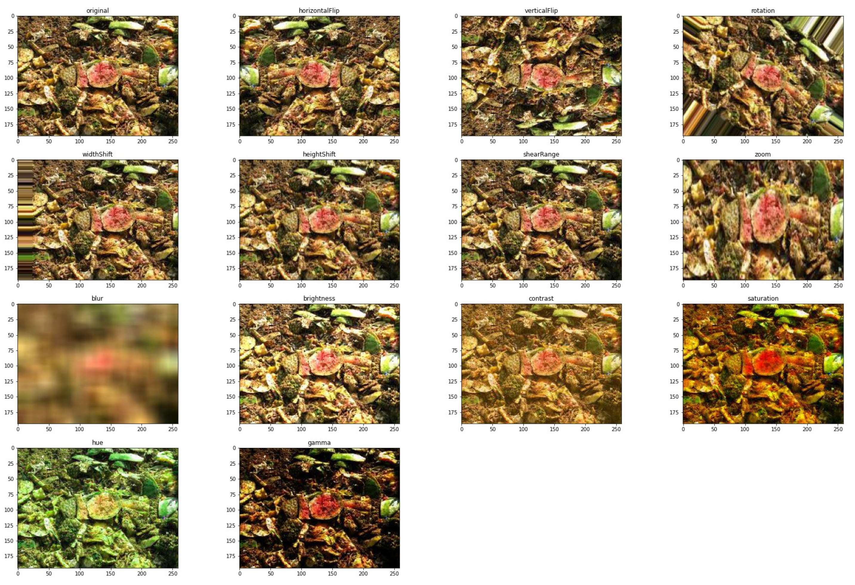
Image augmentation is a useful technique used to increase the diversity of the training dataset such that realistic but random copies of the original image can be generated through simple transformations such as geometric and colour space changes, image cropping, noise injection, and random erasing. By expanding limited datasets, this procedure takes advantage of the capabilities of big data and is known to improve model performance [25]. The augmentation presented in this paper is based on the ImageDataGenerator class provided by the Keras deep learning neural network library [34,58]. Specifically, we used the ImageDataGenerator class to perform 13 transformations on the images (i.e., image rotation and height and width shift); 6 geometric transformations (i.e., horizontal and vertical flip), 5 colour transformations (i.e., contrast, brightness, hue, saturation, and gamma); and 2 additional image manipulations (zoom and blur). The geometric transformations allows for images to be captured in different angles. The colour transformations were deemed necessary to simulate different exposition and luminosity conditions. For the colour transformations, we used only those that do not change the image too much. Default configurations of the ImageDataGenerator class were used for all the transformations, including: image rotation range angle; horizontal and vertical flip allowed; 0.2 width shift range; 0.2 shear range; 0.2 zoom range; 0.2 height shift range (with fill in nearest mode); blur filter enabled; [1.1, 1.5] brightness range; 0.1 hue; 0.5 contrast; 3 saturation; and 2 gamma. These default values can be modified in the image augmentation Python code released with this paper. Some examples of the augmented images are shown in Figure 1, where the top left image represents the original and the rest are augmented images labelled according to the transformation applied.
3.3. Method
We performed image classification tasks on the experimental data with the aim of finding the class (i.e., organic or recyclable) to which a new ‘unseen’ observation belongs. As noted in Section 2, standard machine learning methods such as SVM, decision trees, K-Nearest Neighbour (k-NN), etc. have been applied to classify images with varying levels of success. However, more recent methods such as deep neural network, especially CNN, have proven more successful for image classification [12,14]. In particular, CNN architectures such as VGGNet [19], AlexNet [20], ResNet [21], and DenseNet [22] have proven successful for image classification with high . However, models trained with these standard architectures take a large amount of system resources because they are often pre-trained for more than one purpose, which makes them inefficient in terms of model size and development time when dealing with specific requirements such as the waste image classification task presented in this paper. Thus, we developed a bespoke 5-layer CNN architecture presented in Figure 2.
To investigate the possibility of training an efficient light-weight model with performance and less computational/resource demand, the CNN architecture was trained with two different pixel sizes— and pixels—of the augmented version of Sekar’s [24] waste classification dataset described in Section 3.2. As background, the predominant image resolution size in the original dataset is , hence the selection. However, the smaller resolution size of pixels was chosen arbitrarily. We considered downsizing the original images for the following reasons:
- To show how image resizing can be used to address the requirements of different applications, namely: a light-weight application for low-cost device with limited memory capacity and low-resolution camera and a robust application using high-resolution camera without memory restriction.
- To investigate the variation in performance between the two models. The idea is to determine if smaller image resolution can achieve a relatively high performance, thus avoiding unnecessary waste of system resources in terms of model size and computational time.
We also trained a random guess classifier which forms the baseline against which the performance of our bespoke CNN models was compared. This was deemed necessary due to the absence of ‘reliable’ and ‘reproducible’ existing work to perform a direct comparison. All experiments were conducted in 50 epochs to obtain the best parameter sets. Performance evaluation was based on and cross-entropy observed during model training, validation, and testing.
In classification tasks, metric calculates how often predictions equals class labels [34,35]. Its value can be represented mathematically as Equation (1):
where is the number of positive instances predicted correctly; is the number of negative instances predicted correctly; is the number of positive instances predicted incorrectly; and is the number of negative instances predicted incorrectly.
Cross-entropy is a common function used to optimise and evaluate classification models because its value reveals the magnitude of predicted probability divergence from the actual class labels. This value is pegged on the understanding of Softmax activation function that is usually placed at the end of CNN architectures to convert output logits (i.e., unnormalised predictions) into classification probabilities. For binary classification tasks, cross-entropy is defined mathematically as Equation (2):
where is the truth value taking a value 0 or 1 and is the Softmax probability for the ith class.
3.4. Experimental Setup
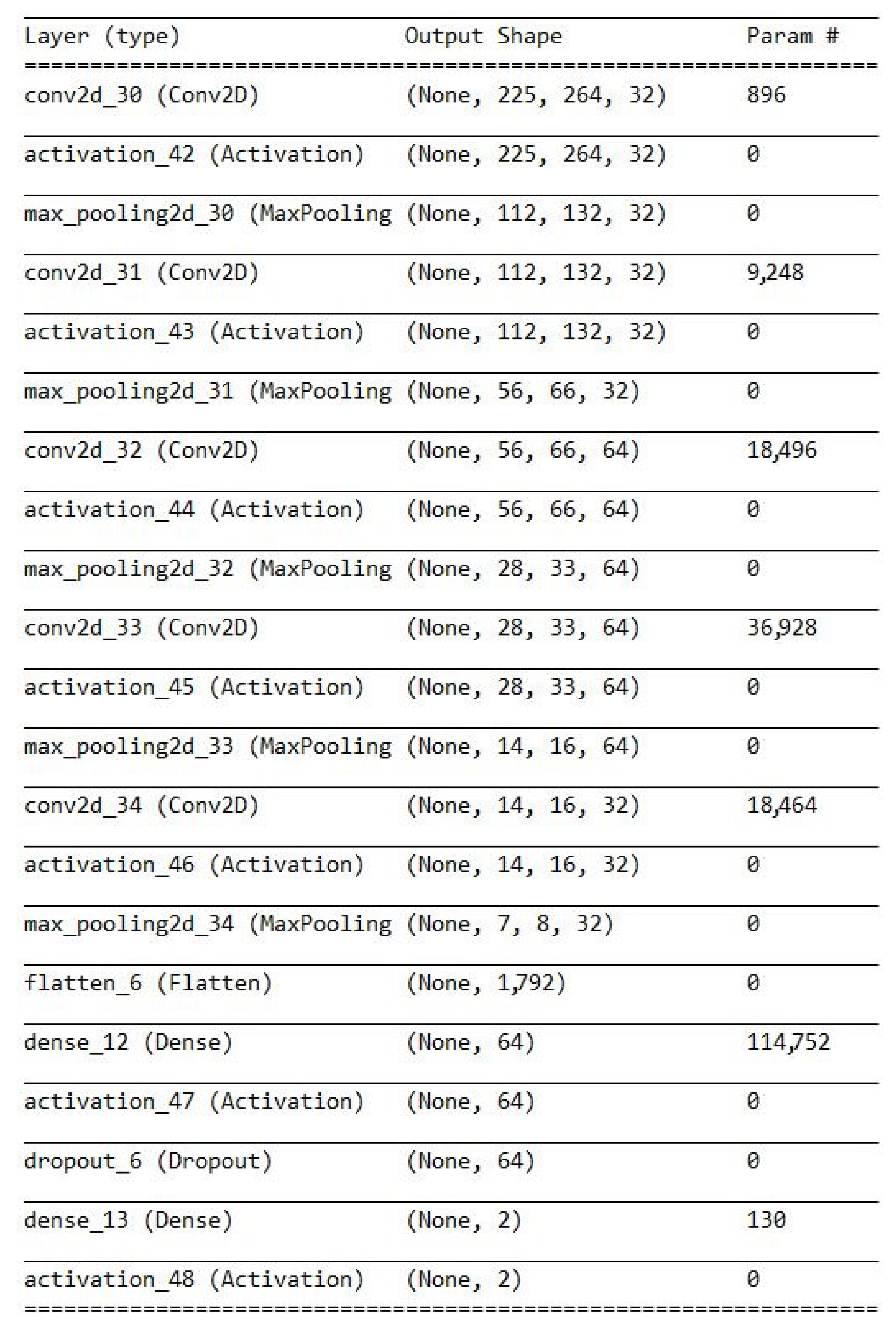
The bespoke CNN architecture is presented in Figure 2, comprising a series of convolutions, plus activation and pooling operations, followed by a number of fully connected layers. Specifically, the CNN consists of 5 convolutional 2D layers of various neuron sizes, each with a ReLu activation function and 2D max pooling of window size. The output of the convolution plus pooling operations is flattened and fed into 2 dense (fully connected) layers, with ReLu and softmax activation function, respectively. A dropout layer of value 0.5 is inserted between the dense layers to classify the given input training images into 2 full level classes. Dropout is by far the most popular regularisation technique for deep neural networks [65] and is known to add a fairly substantial gain to the model . It also prevents over-fitting, because a neuron is temporarily ‘dropped’ or disabled with probability p at each iteration during training. This means that all the inputs and outputs to this neuron will be disabled at the current iteration and resampled with probability p at every training step. In other words, a dropped out neuron at one iteration can be active at the next one. The hyperparameter p, commonly called dropout-rate, is typically defined as a number between 0.0 (no outputs from the layer) and 1.0 (no dropout). Dropout values between between 0.5 and 0.8 are recommended for a hidden layer [66] so we used 0.5 for our CNN architecture. This corresponds to 50% of the neurons being dropped out during training.
The initial input size shown in Figure 2 refers to the maximum input resolution (i.e., ) for the augmented dataset used to train the larger model. The same architecture, with smaller image resolution (i.e., ), was used for training the smaller model. The number of epochs used to train the network is 50 for all experiments (including the baseline). The training, validation, and testing experiments were performed on the augmented dataset split into 60% training, 15% validation, and 25% testing as shown in Table 2.
Deep neural networks are trained based on the stochastic gradient descent optimisation algorithm, so error for the current state of the network is repeatedly estimated as part of the optimisation algorithm. This means that an error function (known as function) must be defined for estimating the of the model at each training iteration so that the weights can be updated to reduce the on the next evaluation. More importantly, the chosen function must be appropriate for the modelling task, in our case classification, and the output layer configuration must match the chosen function [67].
For the bespoke CNN architecture implemented in this paper, we used Keras built-in methods [35] for evaluation including and function. Specifically, we used the cross-entropy which is the default function for classification problems. In Keras, this is specified by compiling the trained model with categorical cross-entropy. Cross-entropy calculates a score that summarises the average difference between the actual and predicted probability distributions for all classes in the problem. The score is then minimised, and a perfect cross-entropy value is 0. For model optimisation, we used the Adadelta algorithm with a learning rate of 1.0 to match the exact form in Zeiler’s original paper [68]. We specified and as the performance metrics.
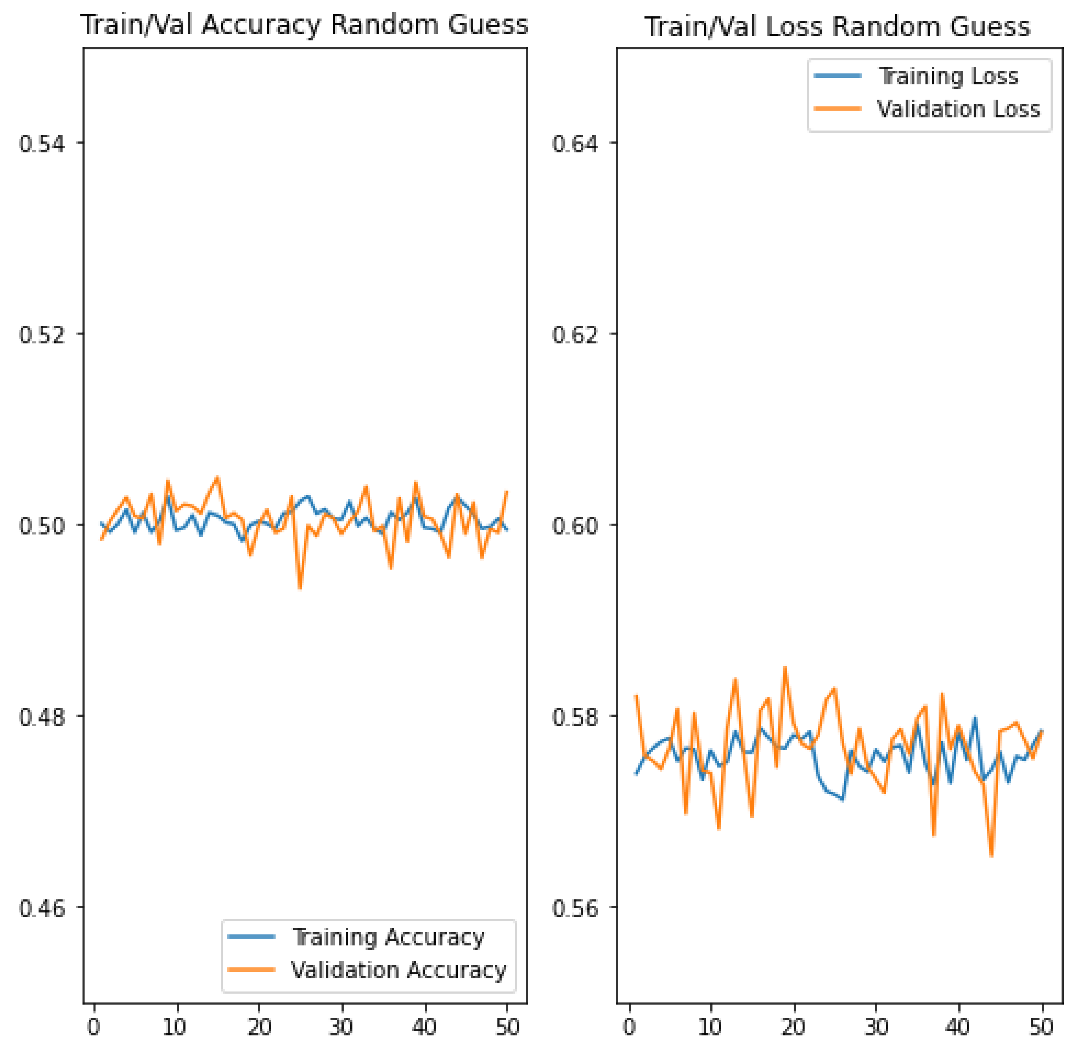
The baseline model used for comparison was implemented by simply replacing the Softmax output probabilities from the CNNs with randomly generated floating point values between 0 and 1. This was repeated 50 times for each experiment to mimic the number of epochs used in the CNN experiments. We did not report development time and model size for the baseline model because it is impractical and unnecessary.
4. Results
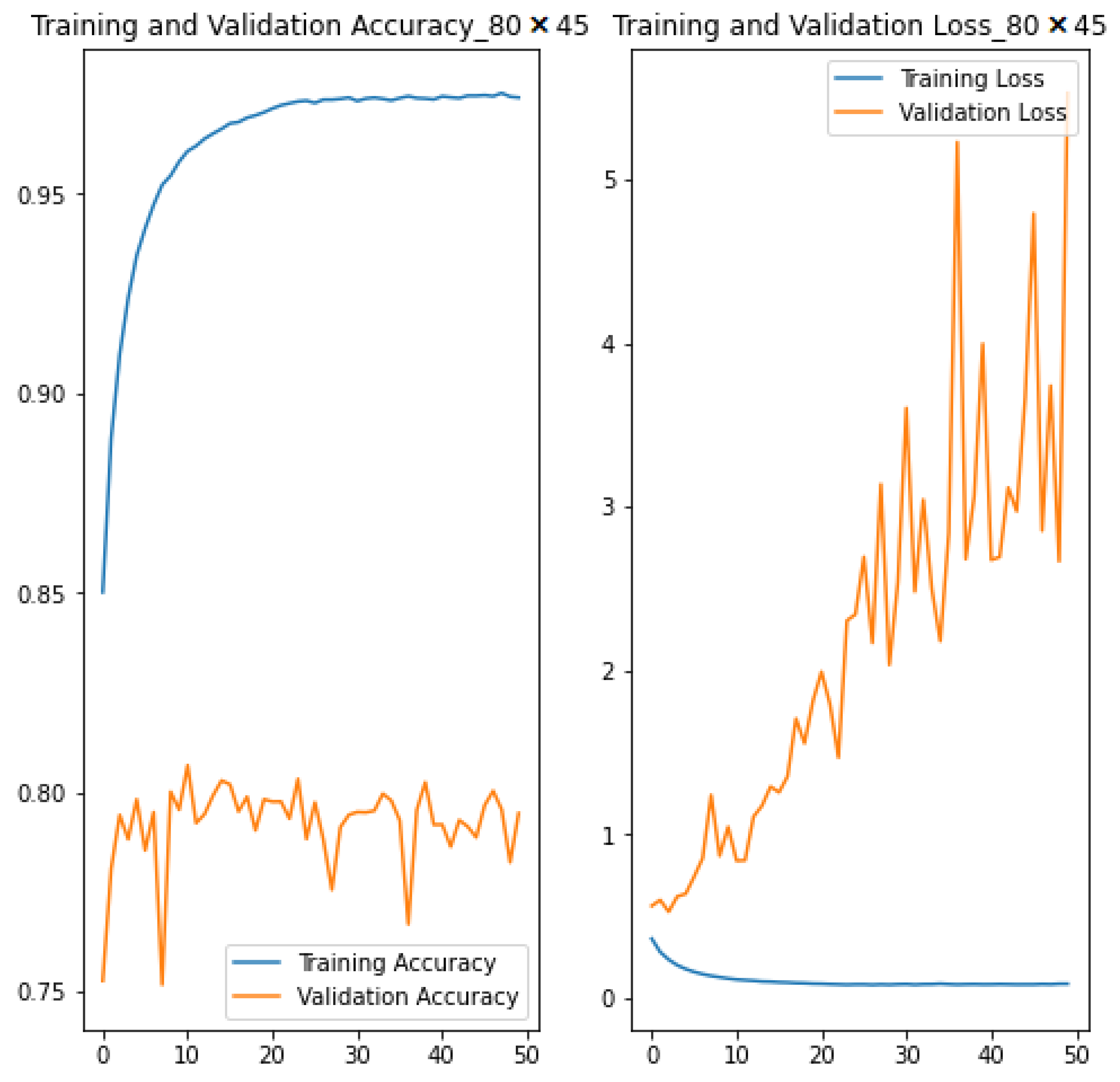
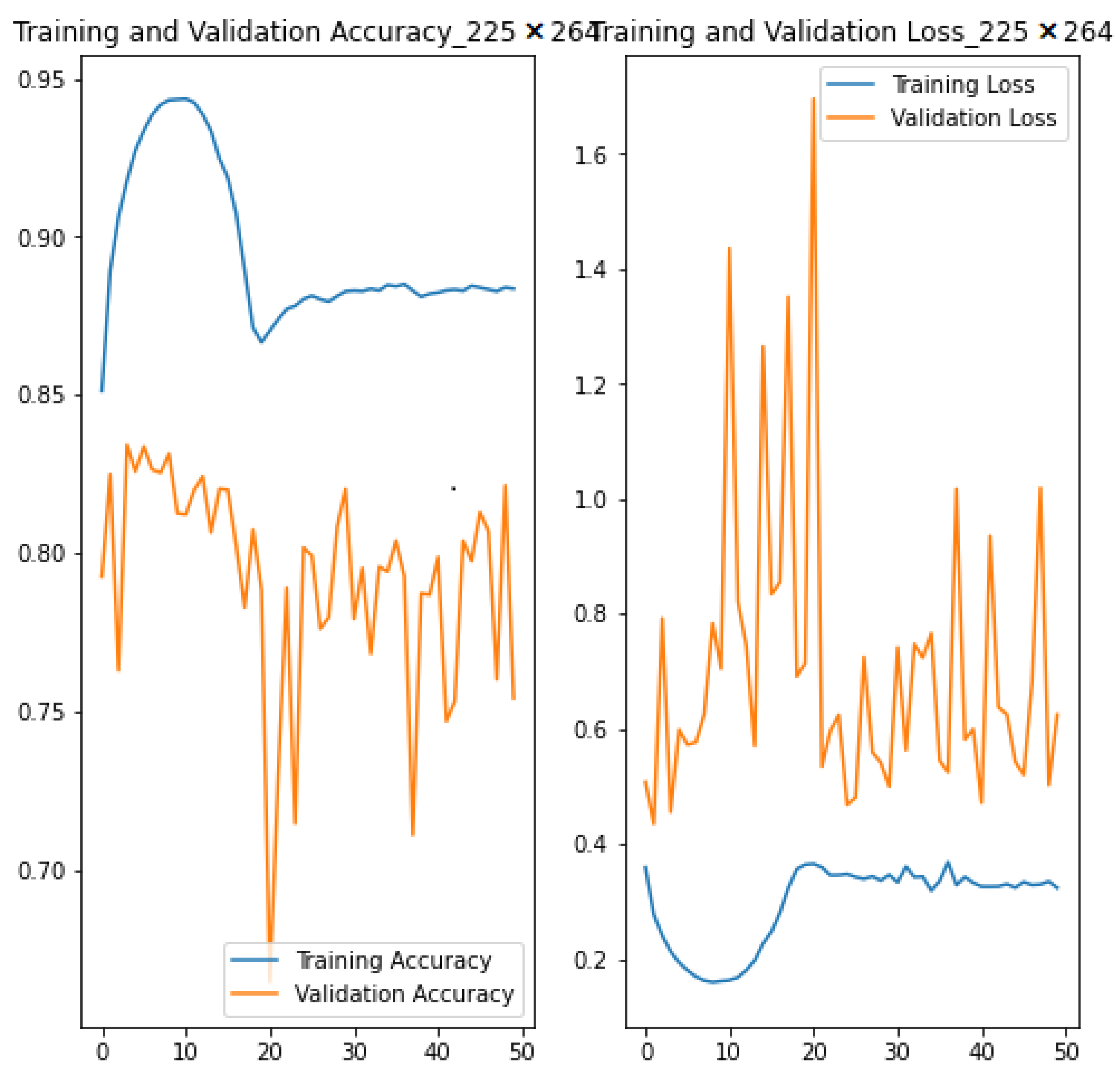
In this section, we present the results obtained from the baseline model as well as the bespoke CNN architecture trained with small () and large () image resolutions. Aggregate measures derived from compiling the models were used for evaluation such as training, validation, and testing and . For simplicity, the performance of the three models are reported together in Table 3. However, the visualisation of the results is represented separately for each model. Figure 3 shows the training/validation and in function of 50 epochs for the smaller model (trained with image resolution), while Figure 4 and Figure 5 show that of the larger model (trained with image resolution) and baseline model, respectively.
As shown in Table 3, the small CNN model with image resolution is relatively lighter than the large model by 1.27MB. The training time is also better with the small model (6.40 h), compared to the large model which took 65.46 h to train. This is particularly important when considering the type of application to deploy the model. For example, the small model would be suitable for embedded applications on low-cost devices with a low-resolution camera and/or limited memory size. On the other hand, the large model is memory demanding and would suit applications with high-resolution camera and no memory size constraints. Computational cost calculation for the baseline model is impractical, so we did not compare the baseline with our approach in terms of development time and model size. Direct comparison with standard CNN architectures such as VGGNet [19], AlexNet [20], ResNet [21], and DenseNet [22] was also deemed unnecessary for the research presented in this paper due to the following reasons:
- The standard CNN architectures were developed as part of the annual ImageNet Large Scale Visual Recognition Challenge (ILSVRC) [69], where researchers compete to correctly detect and/or classify objects and scenes in a large database consisting of 14,197,122 images organised into 21,841 categories. As such, the pre-trained models are inherently very large.
- Self-reported model size and development time will vary among research studies due to variations in the computer system specification, purpose of experiments, data size, etc. For example, Hang et al. [23] used nine standard CNN architectures (with some modifications, such as layer freezing) to classify plant leaf diseases, and compared model size and training time. InceptionNet-v2 [46] produced the smallest model size of 45.1 MB within 2187.3 s. This is super-fast when compared to the 6.40 h used to train our smaller bespoke CNN model that is only 1.08 MB. Their experiment was faster due to higher system specification (i.e., i7-8700k processor and 32GB RAM, accelerated by two NVIDIA GTX 1080TI GPUs).
Based on these reasons, we believe that models trained with the standard CNN architectures are unlikely to result in lower model size and computational cost than our bespoke CNN models, even if they are modified and self-implemented with the experimental dataset used in this paper.
In terms of , our approach performed better than the baseline model, which produced 50.05% during training, validation, and testing. Thus, emphasis in this section is on the comparative performance between the CNN models. The smaller CNN model is generally more accurate than the larger one during training, validation, and testing. Specifically, the smaller model is 6.72% more accurate during training and 4.69% during testing. However, both models produced the same (79.21%) during validation. An important variation to note is the margin between training, validation, and testing per model, as huge differences may indicate how generalisable (or not) a models is. For example, the variation between validation and testing is minimal for both CNN models. In particular, the small model is 1.67% more accurate during testing than validation, but the large model degraded by 3.02% during testing than validation. The ‘training to validation’ and ‘training to testing’ variation is much higher for both models, which provokes an interesting discussion. For the large module, reduced by 10.35% from training to validation and 13.37% from training to testing. The small model exhibited a similar pattern, but with even larger reduction from ‘training to validation’ (17.07%) and ‘training to testing’ (14.40%). These variations can be seen clearly in Figure 3 and Figure 4 for the large and small models, respectively.
There are many reasons why CNN models exhibit this behaviour, ranging from over-fitting to model complexity; it could even be due to unrepresentative training, validation, and/or testing data. The model’s ability to adapt properly to new data (i.e., generalisation) is highly influenced by how similar or dissimilar the unseen data, drawn from the same distribution, are from the one used to train the model. The function usually helps to unravel the reasons for fluctuating values from ‘training to validation to testing’. For example, observed in the small model increased exponentially from training (0.1073) to validation (2.1885) to testing (5.4401). However, observed in the large model increased from training (0.2954) to validation (0.7083), but decreased to 0.5692 during testing. These observations are certainly not the classic case of ‘ decreases while increases’, and the various reasons for this are discussed further in Section 5.
5. Discussion
In order to understand the fluctuations in and values observed in Section 4, it is important to explain the relationship dynamics between and . Intuitively, and are believed to be inversely correlated, where lower and higher should lead to better predictions. However, this is not the case in Table 3, where the smaller model with higher led to higher and better prediction than the larger model. Although surprising, this is not unheard of, as and are not necessarily exactly inversely correlated. While is a measure of the variation between class labels (0 or 1) and the raw prediction (which is typically a float), measures the difference between class labels and threshold prediction (also represented as 0 or 1). Therefore, raw prediction changes exponentially with , but is more ‘resilient’ because raw predictions will have to go over/under a certain threshold to actually affect the value.
To put this into context, let us consider the binary classification performed in the experiment, where the task is to predict whether an image is organic or recyclable waste. The raw prediction of the CNN is a sigmoid (outputting a float between 0 and 1), but the CNN is trained to output 1 if the image belongs to organic waste and 0 otherwise. In the results shown in Figure 3, two phenomena are happening at the same time, i.e., the classic ‘ decreases while increases’ and the less classic ‘ increases while stays the same’. In the earlier phenomenon, some images with borderline predictions may be predicted better, and so the output class changes (e.g., an organic image whose prediction was 0.4 becomes 0.6). This is the classic ‘ decreases while increases’ behaviour that is usually expected. However, some images with very poor predictions may continue to worsen (e.g., an organic image whose prediction was 0.3 becomes 0.2). This leads to the less classic ‘ increases while stays the same’ phenomenon. It is also important to note that when cross-entropy is used for classification (as is the case with the experiments presented in this paper), bad predictions are penalised much more strongly than good predictions are rewarded. Thus, for an organic image, the is log(1—prediction), which means that, even if many organic images are correctly predicted (low ), a single misclassified organic image will have a high , hence disproportionately increasing the mean . This phenomena has been illustrated by other researchers [70] to show that increasing and stable could also be caused by good predictions being classified a little worse.
The second phenomenon ( increases while stays the same) is more likely the case with the large model and less likely with the small model due to the level of ‘ to ’ asymmetry observed in Figure 3 vs. Figure 4. For the small CNN model shown in Figure 3, both and are increasing, which may indicate that the CNN is starting to over-fit, especially because both phenomena are happening at the same time. Specifically, the CNN seem to be learning patterns only relevant for the training set and not great for generalisation (classic phenomena) where some images from the validation set are being predicted really wrong, which has an amplified effect on the ‘ asymmetry’. At the same time, the CNN is still learning some patterns which are useful for generalisation (less classic phenomena) as more images are being correctly classified. In such cases, dropout usually helps in generalising the model. The bespoke CNN architecture presented in this paper uses a dropout of 0.5 (for both large and small models) which means that 50% of the network neurons are dropped during training whereas all the neurons are used for validation. A less aggressive dropout below 0.5 may bring the training and validation much closer, thus making the model more accurate during testing. That said, the asymmetry observed in the small model (Figure 3) may also be due to other factors, such as model complexity and unrepresentative validation data. In the former case, the model may be too complicated for the task, and perhaps a reduction in the depth (number) of layers may resolve the problem. In the latter case, the training data may be unrepresentative compared to the validation data. The recommended solutions to such problems are to randomise the training–validation and testing data split and increase the experimental dataset, respectively. This seems very unlikely to be the cause of the problem in our experiments, because both recommendations have already been applied—the split (60% training, 15% validation, and 25% testing) was randomly drawn from the experimental data, and augmentation was used to increase the original dataset from 24,705 to 345,870 images as reported in Table 1. A possible observation from the literature (not taken into consideration in our experiments) is that some researchers [18] have discredited the original dataset as relatively confusing, with some images either being mislabelled and/or having multiple labels between organic and recyclable. This and other factors related to reducing model complexity and tuning the dropout will be investigated in future research.
The larger model (although less accurate) seems more generalisable based on the observations in Figure 4. The CNN exhibited only the less classic ‘ decreases while stays the same’ behaviour. Specifically, the CNN peaked at epoch 9, with training (0.1591) and (0.9432), and validation (0.7830) and (0.8314). It is very common for researchers to apply early stoppage to their code at this point, thus leading to higher performance being reported. However, both training and validation seem to be going high at this point, which means that the model was probably over-fitting. The model seemed to stabilise around epoch 19 (training : 0.3558, training : 0.8712, validation : 0.6905, and validation : 0.8074) with the odd spikes in and . Indeed, the validation and values obtained at this point seem much closer to the overall results obtained during testing, as shown in Table 3. This shows that the large model is more robust and generalisable compared to the small model. Therefore, future research and experimentation is required to improve the effectiveness and generalisability of the proposed framework of the small model to achieve a balance between and .
6. Conclusions
We have investigated the automation of waste classification by evaluating the performance of a bespoke CNN architecture trained on two different image resolutions of Sekar’s [24] dataset available on Kaggle. We acknowledge that several research works have been reported in this area that utilised the same dataset, but none to our knowledge has been explicit about their experimental setup, or provided source code which allows for their results to be replicated. As such, we implemented a random guess classifier which forms a baseline against which the performance of our approach was compared. As the task is a binary-class one involving a modest dataset size of 24,705 images, we used augmentation to increase the dataset to 345,870. We investigated the performance of two image resolution sizes of the dataset (large model: and small model: ) and compared the results. Our experiments show that the bespoke CNN performed better than the baseline classifier. The small model is relatively lighter than the large model by 1.27 MB, and the training time is also better with the small model (6.40 h) compared to the large model, which took 65.46 h to train. This means that the small model would be suitable for embedded applications on low cost devices with a low-resolution camera and/or limited memory size. On the other hand, the large model is memory demanding and would suit applications with high-resolution camera and no memory size constraints.
In terms of , the small model also performed better than the large one, but the large model seem more generalisable. However, the results obtained in the small model might just be a signal to the model complexity and/or original data veracity. For example the model might be too complex for the classification task, and literature evidence suggests that some images in the original data are either mislabelled and/or have multiple labels between organic and recyclable. In future work, a deeper analysis would be performed on the experimental data to identify and remove any mislabelled images before re-training the model. We will also consider various parameter tuning such as increasing the epoch and using a less aggressive dropout below the 50% currently in place.
Author Contributions
Conceptualisation, formal analysis, investigation, resources, writing—original draft preparation, review and editing, supervision, and project administration, N.N.; methodology, software, validation, data curation, and visualisation, J.B. and J.P. All authors have read and agreed to the published version of the manuscript.
Funding
This research received no external funding.
Institutional Review Board Statement
Not applicable.
Informed Consent Statement
Not applicable.
Data Availability Statement
The original data used for this research are freely available on Kaggle (www.kaggle.com/techsash/waste-classification-data accessed on 24 January 2022). However, the dataset was not used in its original form as further processing, described in Section 3.1 and Section 3.2, was required. To encourage reproducibility of the experiments and results reported in Section 4, the modified data—a Jupyter notebook (.ipynb) file useful to apply data augmentation on the dataset and a Jupyter notebook (.ipynb) file useful to replicate the experiments—has been provided at [37].
Conflicts of Interest
The authors declare no conflict of interest.
References
- Meng, X.; Tan, X.; Wang, Y.; Wen, Z.; Tao, Y.; Qian, Y. Investigation on decision-making mechanism of residents’ household solid waste classification and recycling behaviors. Resour. Conserv. Recycl. 2019, 140, 224–234. [Google Scholar] [CrossRef]
- Guo, X.-x.; Liu, H.-t.; Zhang, J. The role of biochar in organic waste composting and soil improvement: A review. Waste Manag. 2020, 102, 884–899. [Google Scholar] [CrossRef] [PubMed]
- Sharma, B.; Vaish, B.; Monika; Singh, U.K.; Singh, P.; Singh, R.P. Recycling of Organic Wastes in Agriculture: An Environmental Perspective. Int. J. Environ. Res. 2019, 13, 409–429. [Google Scholar] [CrossRef]
- Dhiman, S.S.; Shrestha, N.; David, A.; Basotra, N.; Johnson, G.R.; Chadha, B.S.; Gadhamshetty, V.; Sani, R.K. Producing methane, methanol and electricity from organic waste of fermentation reaction using novel microbes. Bioresour. Technol. 2018, 258, 270–278. [Google Scholar] [CrossRef]
- Taleb, M.A.; Al Farooque, O. Towards a circular economy for sustainable development: An application of full cost accounting to municipal waste recyclables. J. Clean. Prod. 2021, 280, 124047. [Google Scholar] [CrossRef]
- Ferronato, N.; Torretta, V. Waste Mismanagement in Developing Countries: A Review of Global Issues. Int. J. Environ. Res. Public Health 2019, 16, 1060. [Google Scholar] [CrossRef] [Green Version]
- Dzhanova, Y. Sanitation Workers Battle Higher Waste Levels in Residential Areas as Coronavirus Outbreak Persists; CNBC Politics: New York, NY, USA, 2020; Available online: https://www.cnbc.com/2020/05/16/coronavirus-sanitation-workers-battle-higher-waste-levels.html (accessed on 21 January 2022).
- Kaza, S.; Yao, L.C.; Bhada-Tata, P.; Van Woerden, F. What a Waste 2.0: A Global Snapshot of Solid Waste Management to 2050; Urban Development: Washington, DC, USA, 2018. [Google Scholar]
- Yadav, H.; Kumar, P.; Singh, V.P. Hazards from the Municipal Solid Waste Dumpsites: A Review. In Proceedings of the 1st International Conference on Sustainable Waste Management through Design; Springer: Cham, Switzerland, 2019; Volume 21, pp. 336–342. [Google Scholar] [CrossRef]
- Forti, V.; Balde, C.P.; Kuehr, R.; Bel, G. The Global E-Waste Monitor 2020: Quantities, Flows and the Circular Economy Potential; United Nations University/United Nations Institute for Training and Research: Bonn, Germany; International Telecommunication Union: Geneva, Switzerland; International Solid Waste Association: Rotterdam, The Netherland, 2020. [Google Scholar]
- Ellen MacArthur Foundation. The New Plastics Economy: Rethinking the Future of Plastics and Catalysing Action. Available online: https://emf.thirdlight.com/link/cap0qk3wwwk0-l3727v/@/#id=1 (accessed on 21 January 2022).
- Xia, W.; Jiang, Y.; Chen, X.; Zhao, R. Application of machine learning algorithms in municipal solid waste management: A mini review. Waste Manag. Res. J. Sustain. Circ. Econ. 2021, 0734242X2110337. [Google Scholar] [CrossRef]
- Li, W.; Tse, H.; Fok, L. Plastic waste in the marine environment: A review of sources, occurrence and effects. Sci. Total Environ. 2016, 566–567, 333–349. [Google Scholar] [CrossRef]
- Ye, Z.; Yang, J.; Zhong, N.; Tu, X.; Jia, J.; Wang, J. Tackling environmental challenges in pollution controls using artificial intelligence: A review. Sci. Total Environ. 2020, 699, 134279. [Google Scholar] [CrossRef]
- LeCun, Y.; Bengio, Y.; Hinton, G. Deep learning. Nature 2015, 521, 436–444. [Google Scholar] [CrossRef]
- Sun, Y.; Xue, B.; Zhang, M.; Yen, G.G. Evolving Deep Convolutional Neural Networks for Image Classification. IEEE Trans. Evol. Comput. 2020, 24, 394–407. [Google Scholar] [CrossRef] [Green Version]
- Rawat, W.; Wang, Z. Deep Convolutional Neural Networks for Image Classification: A Comprehensive Review. Neural Comput. 2017, 29, 2352–2449. [Google Scholar] [CrossRef] [PubMed]
- Liang, S.; Gu, Y. A deep convolutional neural network to simultaneously localize and recognize waste types in images. Waste Manag. 2021, 126, 247–257. [Google Scholar] [CrossRef] [PubMed]
- Simonyan, K.; Zisserman, A. Very Deep Convolutional Networks for Large-Scale Image Recognition. arXiv 2014, arXiv:1409.1556. [Google Scholar]
- Krizhevsky, A.; Sutskever, I.; Hinton, G.E. ImageNet Classification with Deep Convolutional Neural Networks. In Advances in Neural Information Processing Systems; Pereira, F., Burges, C.J.C., Bottou, L., Weinberger, K.Q., Eds.; Curran Associates, Inc.: Vancouver, BC, Canada, 2012; Volume 25. [Google Scholar]
- He, K.; Zhang, X.; Ren, S.; Sun, J. Deep Residual Learning for Image Recognition. arXiv 2015, arXiv:1512.03385. [Google Scholar]
- Huang, G.; Liu, Z.; van der Maaten, L.; Weinberger, K.Q. Densely Connected Convolutional Networks. arXiv 2016, arXiv:1608.06993. [Google Scholar]
- Hang, J.; Zhang, D.; Chen, P.; Zhang, J.; Wang, B. Classification of Plant Leaf Diseases Based on Improved Convolutional Neural Network. Sensors 2019, 19, 4161. [Google Scholar] [CrossRef] [Green Version]
- Sekar, S. Waste Classification Data, Version 1. Available online: https://www.kaggle.com/techsash/waste-classification-data (accessed on 18 January 2022).
- Shorten, C.; Khoshgoftaar, T.M. A survey on Image Data Augmentation for Deep Learning. J. Big Data 2019, 6, 60. [Google Scholar] [CrossRef]
- Toğaçar, M.; Ergen, B.; Cömert, Z. Waste classification using AutoEncoder network with integrated feature selection method in convolutional neural network models. Measurement 2020, 153, 107459. [Google Scholar] [CrossRef]
- Mulim, W.; Revikasha, M.F.; Rivandi; Hanafiah, N. Waste Classification Using EfficientNet-B0. In Proceedings of the IEEE Institute of Electrical and Electronics Engineers, Jakarta, Indonesia, 28 October 2021; pp. 253–257. [Google Scholar] [CrossRef]
- Mallikarjuna, M.G.; Yadav, S.; Shanmugam, A.; Hima, V.; Suresh, N. Waste Classification and Segregation: Machine Learning and IOT Approach; Institute of Electrical and Electronics Engineers Inc.: New York, NY, USA, 2021; pp. 233–238. [Google Scholar] [CrossRef]
- Gupta, T.; Joshi, R.; Mukhopadhyay, D.; Sachdeva, K.; Jain, N.; Virmani, D.; Garcia-Hernandez, L. A deep learning approach based hardware solution to categorise garbage in environment. Complex Intell. Syst. 2021, 1–24. [Google Scholar] [CrossRef]
- Masand, A.; Chauhan, S.; Jangid, M.; Kumar, R.; Roy, S. ScrapNet: An Efficient Approach to Trash Classification. IEEE Access 2021, 9, 130947–130958. [Google Scholar] [CrossRef]
- Hoque, M.A.; Azad, M.; Ashik-Uz-Zaman, M. IoT and Machine Learning Based Smart Garbage Management and Segregation Approach for Bangladesh; Institute of Electrical and Electronics Engineers Inc.: New York, NY, USA, 2019. [Google Scholar] [CrossRef]
- Mollá, I.F. Inorganic Waste Classifier Using Artificial Intelligence. Ph.D. Thesis, LAB University of Applied Sciences, Lahti, Finland, 2021. [Google Scholar]
- Faria, R.; Ahmed, F.; Das, A.; Dey, A. Classification of Organic and Solid Waste Using Deep Convolutional Neural Networks. In Proceedings of the 2021 IEEE 9th Region 10 Humanitarian Technology Conference (R10-HTC), Bangalore, India, 30 September–2 October 2021; pp. 1–6. [Google Scholar] [CrossRef]
- Chollet, F. Deep Learning with Python, 1st ed.; Manning Publications: Shelter Island, NY, USA, 2018. [Google Scholar]
- Chollet, F. Training and Evaluation with the Built-In Methods. Available online: https://keras.io/guides/training_with_built_in_methods/ (accessed on 20 January 2022).
- Murphy, K.P. Machine Learning: A Probabilistic Perspective. In Adaptive Computation and Machine Learning Series; Bach, F., Ed.; MIT Press: London, UK, 2012. [Google Scholar]
- Nnamoko, N.; Barrowclough, J.; Procter, J. Waste Classification Dataset. Mendeley Data 2022, V2. [Google Scholar] [CrossRef]
- Zhao, Z.Q.; Zheng, P.; Xu, S.T.; Wu, X. Object Detection With Deep Learning: A Review. IEEE Trans. Neural Netw. Learn. Syst. 2019, 30, 3212–3232. [Google Scholar] [CrossRef] [Green Version]
- Long, J.; Shelhamer, E.; Darrell, T. Fully convolutional networks for semantic segmentation. In Proceedings of the 2015 IEEE Conference on Computer Vision and Pattern Recognition (CVPR), Boston, MA, USA, 7–12 June 2015; pp. 3431–3440. [Google Scholar] [CrossRef] [Green Version]
- Xie, S.; Girshick, R.; Dollár, P.; Tu, Z.; He, K. Aggregated Residual Transformations for Deep Neural Networks. In Proceedings of the IEEE Conference on Computer Vision and Pattern Recognition, Las Vegas, NV, USA, 26 June–1 July 2016. [Google Scholar]
- Thung, G.; Yang, M. Classification of Trash for Recyclability Status; Leland Stanford Junior University: Palo Alto, CA, USA, 2016; Available online: http://cs229.stanford.edu/proj2016/report/ThungYang-ClassificationOfTrashForRecyclabilityStatus-report.pdf (accessed on 19 January 2022).
- Srinilta, C.; Kanharattanachai, S. Municipal Solid Waste Segregation with CNN. In Proceedings of the 2019 5th International Conference on Engineering, Applied Sciences and Technology (ICEAST), Luang Prabang, Laos, 2–5 July 2019; pp. 1–4. [Google Scholar] [CrossRef]
- Sandler, M.; Howard, A.; Zhu, M.; Zhmoginov, A.; Chen, L.C. MobileNetV2: Inverted Residuals and Linear Bottlenecks. In Proceedings of the 2018 IEEE/CVF Conference on Computer Vision and Pattern Recognition, Salt Lake City, UT, USA, 18–23 June 2018; pp. 4510–4520. [Google Scholar] [CrossRef] [Green Version]
- Dewulf, V. Application of Machine Learning to Waste Management: Identification and Classification of Recyclables; Technical Report; Imperial College: London, UK, 2017. [Google Scholar]
- Szegedy, C.; Liu, W.; Jia, Y.; Sermanet, P.; Reed, S.; Anguelov, D.; Erhan, D.; Vanhoucke, V.; Rabinovich, A. Going Deeper with Convolutions. arXiv 2014, arXiv:1409.4842. [Google Scholar]
- Szegedy, C.; Vanhoucke, V.; Ioffe, S.; Shlens, J.; Wojna, Z. Rethinking the Inception Architecture for Computer Vision. arXiv 2015, arXiv:1512.00567. [Google Scholar]
- Wang, H.; Li, Y.; Dang, L.M.; Ko, J.; Han, D.; Moon, H. Smartphone-based bulky waste classification using convolutional neural networks. Multimed. Tools Appl. 2020, 79, 29411–29431. [Google Scholar] [CrossRef]
- Castellano, G.; Carolis, B.D.; Macchiarulo, N.; Rossano, V. Learning waste Recycling by playing with a Social Robot. In Proceedings of the 2019 IEEE International Conference on Systems, Man and Cybernetics (SMC), Bari, Italy, 6–9 October 2019; pp. 3805–3810. [Google Scholar] [CrossRef]
- Radhika, D.A. Real Life Smart Waste Management System [Dry, Wet, Recycle, Electronic and Medical]. Int. J. Sci. Res. Sci. Technol. 2021, 7, 631–640. [Google Scholar] [CrossRef]
- Howard, A.G.; Zhu, M.; Chen, B.; Kalenichenko, D.; Wang, W.; Weyand, T.; Andreetto, M.; Adam, H. MobileNets: Efficient Convolutional Neural Networks for Mobile Vision Applications. arXiv 2017, arXiv:1704.04861. [Google Scholar]
- Rahman, M.W.; Islam, R.; Hasan, A.; Bithi, N.I.; Hasan, M.M.; Rahman, M.M. Intelligent waste management system using deep learning with IoT. J. King Saud Univ.—Comput. Inf. Sci. 2020. [Google Scholar] [CrossRef]
- Siva Kumar, A.P.; Buelaevanzalina, K.; Chidananda, K. An efficient classification of kitchen waste using deep learning techniques. Turk. J. Comput. Math. Educ. 2021, 12, 5751–5762. [Google Scholar]
- Kusrini; Saputra, A.P. Waste Object Detection and Classification using Deep Learning Algorithm: YOLOv4 and YOLOv4-tiny. Turk. J. Comput. Math. Educ. 2021, 12, 1666–1677. [Google Scholar]
- Teh, J. Household Waste Segregation Using Intelligent Vision System. Ph.D. Thesis, Universiti Tunku Abdul Rahman, Perak, Malaysia, 2021. Available online: http://eprints.utar.edu.my/4220/ (accessed on 19 January 2022).
- Alonso, S.L.N.; Forradellas, R.F.R.; Morell, O.P.; Jorge-Vazquez, J. Digitalization, circular economy and environmental sustainability: The application of artificial intelligence in the efficient self-management of waste. Sustainability 2021, 13, 92. [Google Scholar] [CrossRef]
- Majchrowska, S.; Mikołajczyk, A.; Ferlin, M.; Klawikowska, Z.; Plantykow, M.A.; Kwasigroch, A.; Majek, K. Deep learning-based waste detection in natural and urban environments. Waste Manag. 2022, 138, 274–284. [Google Scholar] [CrossRef]
- Sivakumar, M.; Renuka, P.; Chitra, P.; Karthikeyan, S. IoT incorporated deep learning model combined with SmartBin technology for real-time solid waste management. Comput. Intell. 2021. [Google Scholar] [CrossRef]
- Chollet, F. Building Powerful Image Classification Models Using Very Little Data. Available online: https://blog.keras.io/building-powerful-image-classification-models-using-very-little-data.html (accessed on 19 January 2022).
- Tan, M.; Le, Q.V. EfficientNet: Rethinking Model Scaling for Convolutional Neural Networks. arXiv 2019, arXiv:1905.11946. [Google Scholar]
- Irving, B. A Gentle Autoencoder Tutorial (with Keras); GitHub: San Francisco, CA, USA, 2016; Available online: https://github.com/benjaminirving/mlseminars-autoencoders/blob/master/Autoencoders.ipynb (accessed on 19 January 2022).
- Alaslani, M.G.; Elrefaei, L.A. Convolutional Neural Network Based Feature Extraction for IRIS Recognition. Int. J. Comput. Sci. Inf. Technol. 2018, 10, 65–78. [Google Scholar] [CrossRef] [Green Version]
- Bansal, V.; Libiger, O.; Torkamani, A.; Schork, N.J. Statistical analysis strategies for association studies involving rare variants. Nat. Rev. Genet. 2010, 11, 773–785. [Google Scholar] [CrossRef] [Green Version]
- Keim, R. Understanding Color Models Used in Digital Image Processing. Available online: https://www.allaboutcircuits.com/technical-articles/understanding-color-models-used-in-digital-image-processing/ (accessed on 19 January 2022).
- Provenzi, E. Color Image Processing; MDPI: Basel, Switzerland, 2018. [Google Scholar] [CrossRef]
- Dertat, A. Applied Deep Learning—Part 4: Convolutional Neural Networks. Available online: https://towardsdatascience.com/applied-deep-learning-part-4-convolutional-neural-networks-584bc134c1e2 (accessed on 19 January 2022).
- Brownlee, J. A Gentle Introduction to Dropout for Regularizing Deep Neural Networks; Publisher: Machine Learning Mastery. 2018. Available online: https://machinelearningmastery.com/dropout-for-regularizing-deep-neural-networks/ (accessed on 19 January 2022).
- Brownlee, J. How to Choose Loss Functions When Training Deep Learning Neural Networks; Publisher: Machine Learning Mastery. 2019. Available online: https://machinelearningmastery.com/how-to-choose-loss-functions-when-training-deep-learning-neural-networks/ (accessed on 19 January 2022).
- Zeiler, M.D. ADADELTA: An Adaptive Learning Rate Method. arXiv 2012, arXiv:1212.5701. [Google Scholar]
- Russakovsky, O.; Deng, J.; Su, H.; Krause, J.; Satheesh, S.; Ma, S.; Huang, Z.; Karpathy, A.; Khosla, A.; Bernstein, M.; et al. ImageNet Large Scale Visual Recognition Challenge. Int. J. Comput. Vis. (IJCV) 2015, 115, 211–252. [Google Scholar] [CrossRef] [Green Version]
- Good Accuracy Despite High Loss Value. Cross Validated. Version: 25 May 2017. Available online: https://stats.stackexchange.com/q/281651 (accessed on 19 January 2022).
Figure 1.
Sample of augmentation for class ‘organic’ including the original and augmented images.

Figure 2.
Bespoke 5-Layer Convolutional Neural Network Architecture.

Figure 3.
Training/validation and for image size .

Figure 4.
Training/validation and for image size .

Figure 5.
Training/validation and for the Baseline classifier (Random Guess).


Table 1.
Characteristics of the original and augmented experimental data.
| Class Name | Class ID | Original Image | Augmented Image |
|---|---|---|---|
| Organic | 1 | 13,880 | 194,320 |
| Recyclable | 0 | 10,825 | 151,550 |
| Total | 24,705 | 345,870 |
Table 2.
Augmented dataset split for training, validation and testing the CNN.
| Class Name | Training | Validation | Testing |
|---|---|---|---|
| Organic | 116,592 | 29,148 | 48,580 |
| Recyclable | 90,930 | 22,732 | 37,888 |
| Total | 207,522 | 51,880 | 86,468 |
Table 3.
Model size, development time, and performance of both models.
| Input Resolution (pixel) | Epochs | Dev. Time (hour) | Model Size (MB) | Loss | Accuracy | ||||
|---|---|---|---|---|---|---|---|---|---|
| Training | Validation | Testing | Training | Validation | Testing | ||||
| 50 | 65.46 † | 2.35 † | 0.2954 | 0.7083 | 0.5692 | 0.8956 | 0.7921 | 0.7619 | |
| 50 | 6.40 † | 1.08 † | 0.1073 | 2.1885 | 5.4401 | 0.9628 | 0.7921 | 0.8088 | |
| Baseline | 50 | - | - | 0.5758 | 0.5768 | 0.5767 | 0.5005 | 0.5005 | 0.5005 |
† System specification used for experiment:- PROCESSOR: Intel(R) Core(TM) i7-10750H CPU @ 2.60GHz; GPU:
NVIDIA GeForce RTX 2070 with Max-Q Design 16GB; RAM: 16GB.
Publisher’s Note: MDPI stays neutral with regard to jurisdictional claims in published maps and institutional affiliations. |
© 2022 by the authors. Licensee MDPI, Basel, Switzerland. This article is an open access article distributed under the terms and conditions of the Creative Commons Attribution (CC BY) license (https://creativecommons.org/licenses/by/4.0/).
Share and Cite
MDPI and ACS Style
Nnamoko, N.; Barrowclough, J.; Procter, J. Solid Waste Image Classification Using Deep Convolutional Neural Network. Infrastructures 2022, 7, 47. https://doi.org/10.3390/infrastructures7040047
AMA Style
Nnamoko N, Barrowclough J, Procter J. Solid Waste Image Classification Using Deep Convolutional Neural Network. Infrastructures. 2022; 7(4):47. https://doi.org/10.3390/infrastructures7040047
Chicago/Turabian StyleNnamoko, Nonso, Joseph Barrowclough, and Jack Procter. 2022. "Solid Waste Image Classification Using Deep Convolutional Neural Network" Infrastructures 7, no. 4: 47. https://doi.org/10.3390/infrastructures7040047