
Developing Bridge Deterioration Models Using an Artificial Neural Network


Department of Civil and Environmental Engineering, The University of Toledo, 2801 Bancroft St, Toledo, OH 43606, USA
*
Author to whom correspondence should be addressed.
Infrastructures 2022, 7(8), 101; https://doi.org/10.3390/infrastructures7080101
Submission received: 20 May 2022
/
Revised: 28 July 2022
/
Accepted: 28 July 2022
/
Published: 31 July 2022
(This article belongs to the Special Issue Resilient Bridge Infrastructures)
Abstract
:The condition of a bridge is critical in quality evaluations and justifying the significant costs incurred by maintaining and repairing bridge infrastructures. Using bridge management systems, the department of transportation in the United States is currently supervising the construction and renovations of thousands of bridges. The inability to obtain funding for the current infrastructures, such that they comply with the requirements identified as part of maintenance, repair, and rehabilitation (MR&R), makes such bridge management systems critical. Bridge management systems facilitate decision making about handling bridge deterioration using an efficient model that accurately predicts bridge condition ratings. The accuracy of this model can facilitate MR&R planning and is used to confirm funds allocated to repair and maintain the bridge network management system. In this study, an artificial neural network (ANN) model is developed to improve the bridge management system (BMS) by improving the prediction accuracy of the deterioration of bridge decks, superstructures, and substructures. A large dataset of historical bridge condition assessment data was used to train and test the proposed ANN models for the deck, superstructure, and substructure components, and the accuracy of these models was 90%, 90%, and 89% on the testing set, respectively.
1. Introduction
Historically, the deterioration of bridges in the United States (US) has been a great challenge. For example, a recent study by the American Society of Civil Engineers (ASCE) identified that there are more than 610,000 bridges in the US and that approximately 9.1% of these bridges are either structurally unsound or not operational [1]. Transportation authorities employ a bridge management system (BMS) to maintain these structures and ensure the safe operation of bridges. A BMS stores inventory data such as inspection data and applies deterioration models to predict future bridge conditions in order to plan maintenance, repair, and rehabilitation (MR&R). This is achieved via the accurate prediction of MR&R operations. BMSs have been used to accurately predict future bridge conditions [2,3]. The Federal Highway Administration (FHWA) has summarized the typical used condition of bridge components on a scale of 0–9, as shown in Table 1.
Each bridge component is deteriorated at a unique rate, independent of other components, as discussed in [4]. Using the BMS deterioration model, it is easy to determine future bridge conditions, and the predicted conditions can be used to facilitate effective decision making and determine appropriate MR&R operations. First, the formulation of deterioration models applied in the infrastructure management system is primarily performed for a pavement management system. We note that these models have been utilized since the 1980s to predict bridge conditions in order to facilitate effective financial estimations of different management methods and select an appropriate method. Generally, all deterioration models are classified into four main categories, i.e., mechanistic, deterministic, stochastic, and artificial intelligence (AI) models.
Mechanistic models are typically well known as those used to predict the operational lifetime of a structure by applying mathematical fundamentals related to the degradation of concrete based on the microstructure of concrete before and during deterioration [5]. Mechanistic models are commonly efficient when applied at the project level other than at the network level [6].
Several studies have employed deterministic models to approximate the forecasted conditions by assuming that there exists some perfect knowledge of variables restricting the approach not to include the random errors in the prediction [7,8]. Most deterministic models use the regression method, where a wide range of mathematical relationships are applied, e.g., exponential decay [9] and polynomial expressions [10,11]. The conditions of a bridge’s superstructure were modeled by applying various functional forms, e.g., linear, nonlinear, nonparametric, and nonlinear parametric, to construct several regression models [12].
Stochastic models allow the formulation of deterioration modeling approaches because various parameters, e.g., randomness and uncertainties, are factored into the deterioration process [13]. In many previous studies, the stochastic Markovian model has been applied extensively when modeling the infrastructure deterioration of bridge components [14]. Several methods have been tested to approximate the probabilities of Markovian transition for a bridge, such as the expected value method approach shown in [15], as well as econometric approaches such as the ordered probity techniques reported in [2,16], count data models, random-effects probit models [17], poisson regression models and negative binomial regression models [2]. Regression-based methods are commonly used [18,19]. However, several studies have proven that regression-based methods introduce bias when predicting future bridge conditions when applying the Markov chain [20].
Bridge deterioration depends upon several factors, e.g., environmental exposure, average daily traffic, design parameters, and other physical bridge properties. Therefore, an accurate prognosis of bridge deterioration is an extremely complicated task. Due to recent advancements in AI models, e.g., machine learning and deep learning, many applications in a wide range of engineering and technology fields are exploiting the benefits of AI models. In addition, large datasets from various fields are available, and such datasets are used to train and test AI models to successfully predict outcomes with sufficient accuracy.
For example, [21] studied a comparison-based convolutional neural networks (CNN) method to determine the state rating of bridge components in the US state of Maryland, and the developed models achieved 86% mean prediction accuracy. In addition, artificial neural network (ANN) applications have been around for approximately 30 years, and ANN models have been used as substitutes for the conventional approaches used in various civil engineering disciplines [22,23,24,25,26,27]. A common ANN approach has been used to model bridge deterioration [28] where a multilayer perceptron (MLP) is employed to establish the association of bridge age (in terms of years) and the bridge condition rating (rated on a scale of 1–9). It was reported that 79% of all predicted values matched the actual values. An ANN-based analysis of historical maintenance combined with inspection records of concrete-built bridge decks in the state of Wisconsin was performed, and this model achieved 75% accuracy in categorizing the state rating [29]. Furthermore, ANNs were applied to ascertain wave loads based on a certified set of data [30]. Here, the ANN approach was used to predict solitary wave forces on a coastal bridge deck. In addition, ANN models were used to estimate bridge damage, and other researchers have modeled the deterioration of a railway bridge in Poland using an ANN to analyze the open decks [31,32,33].
In this study, ANN models were developed to predict the condition ratings of three different bridge components, i.e., the bridge deck, superstructure, and substructure. The proposed models were developed by applying historic bridge condition evaluations from Ohio from 1992 to 2019. With the proposed ANN models, we found that the correlation between the predicted and actual values is high, which demonstrates that the proposed models were able to predict the bridge conditions. The proposed ANN models represent an information-oriented state prediction method for bridge elements with an exemplified forecasting accuracy. In addition, the models were deployed as an information-based modeling method for condition ratings to improve the decision-making processes in a BMS.
2. Methodology
An ANN model uses different mathematical layers to learn various features in the data being processed. Typically, an ANN model comprises thousands to tens of thousands of manmade neurons arranged in layers as units. The input layer is designed to receive multiple types of data and extract various features in the data. The extracted information is then passed to a hidden layer. The feature learning and transformation processes occur in a hidden layer, and the output layer converts the processed information to its original format to facilitate easy interpretation. However, due to the exponential increase in computational power over the last few years, ANN models have evolved to incorporate multiple hidden layers.
In addition, many design optimizations, e.g., architectural variations, and preprocessing techniques are being incorporated into these models. Consequently, these advanced ANN models can produce highly accurate results; thus, ANN researchers can improve their models by performing a variety of simulations based on combining a set of hyperparameters, e.g., the total number of layers (i.e., up to 14 hidden layers) and neurons (i.e., up to 512 neurons), activation functions, biases, and weights.
In this study, TensorFlow and Keras were used to implement the ANN models, and these models were trained and tested on Google’s Colab platform, which has the computational power of several graphical processing units. As a result, the optimal model that can provide the most valuable results can be realized.
2.1. Data Processing
In this study, the data used to formulate the deterioration models of bridge structures were sourced from the National Bridge Inventory (NBI) database. These data include information about the geometric properties of the bridge, i.e., length, width, degree of skew, the operational category of the bridge, road network, type of construction materials, and the type of construction design. The FHWA items from the NBI database are detailed in Table 2.
The National Bridge Inventory (NBI) database is difficult to apply due to the imbalance of data and scattering of information. During the design and implementation phases of the deterioration models, complications were avoided by cleaning the NBI data. This was further facilitated by eliminating the condition rating of the bridge structures, and information about the condition of the missing deck structure, superstructure, and substructure used to train the ANN models. Here, condition ratings that were less than three were eliminated because very few bridge components have a condition under three. In addition, data whose condition rating is denoted N (“Not Applicable”) were also eliminated because they represent culverts, which were considered irrelevant to the current task. After the initial data preparation, erroneous data were also eliminated. The information was verified to eliminate mistakes in the data, e.g., negative age values, negative average daily traffic (ADT) values, and skew angles of 90 degrees. This constraint was used to eliminate most decks, superstructures, and substructures that had undergone repairs. If a bridge’s condition rating increased due to repairs, the condition data after treatment were removed such that only deterioration condition data remained in the dataset.
2.2. Data Standardization
It is beneficial to standardize the input data and output results to prevent calculation hitches, such as features with wider ranges from dominating the distance metric, to satisfy the algorithm states and facilitate the network learning process [34]. Data standardization is the process of converting data categorically and normalizing numerical data. It is imperative to understand data encoding and normalization in the implementation of a neural network model. We note that the total number of nodes located in the layer at the input side of an ANN model is determined by the number of inputs. In addition, the total number of nodes depends on how the input factors are arranged. Here, continuous quantitative variables, e.g., year of construction, age of the structure, and ADT, were applied in a single node. Discrete information identifies the number of nodes that must show a qualitative variable. In this study, the standardization of quantitative variables was performed using the Z-score, which is expressed as follows:
where z is the standardized value, is the nonstandardized value, is the mean value, and is the standard deviation.
We note that the discrete input factors have exclusive categorized classes, where each class is linked to a node in the input layer depending on the various input numbers chosen for various ANN models. The key concept of standardization is that units are dropped randomly for each training iteration. Here, the ANN model showed the corresponding rating of the bridge condition. Regarding the integer scale of the rating system, we considered the output to be a discrete variable and formatted the output in a binary format similar to the discrete input parameters.
In this study, 60% of the dataset was selected randomly without replacement to train the multilayer perceptron (MLP) networks, 20% was selected as the validation set, and 20% was selected as the test set. Here, the data used for testing were meant to approximate the generalizability of the model, and the validation data dictated the model selection and how the model’s parameters were adjusted.
2.3. Multilayer Perceptron
The MLP is type of feedforward Neural Network. Additionally, they are made up of an individual or multiple layers of neurons. A multilayer feedforward neural network that is trained through backpropagation (BP) depends on a controlled technique, i.e., the network formulates the model depending on features input to the system, which is required to establish a connection between the input and output [35]. This MLP enables the prediction of an output that corresponds to particular features of the input feedforward NN such that nonlinearity functions are configured in sequential layers, then into a unidirectional format drawn from the input layer via the hidden layers, and then toward the output layer.
A neuron is applied as an underlying building block in BP networks. Here, a typical neuron is denoted as n and comprises several inputs and a single output which is regarded as an activation state. The computational analysis of a neuron is formulated in Equation (2), where p (i) denotes the activation state, the number of neurons is represented by R, the weight of the neuron is represented by w (i), and the ni represents the outputs from the neuron of the ith example. Here, the activation state is multiplied by the weight. Then, we sum the products and the end sum is denoted as Net, whereas the Net input is estimated in the initial layer of the network as the product (sum) of the source times the weight is added to the bias. Additionally, if the input is significantly greater, the weight has to be exceptionally small in order to avoid the whole transfer function becoming saturated.
After determining Net, F, i.e., an activation function, is employed for the modification purposes of generating an input of the neuron.
2.4. Activation Function
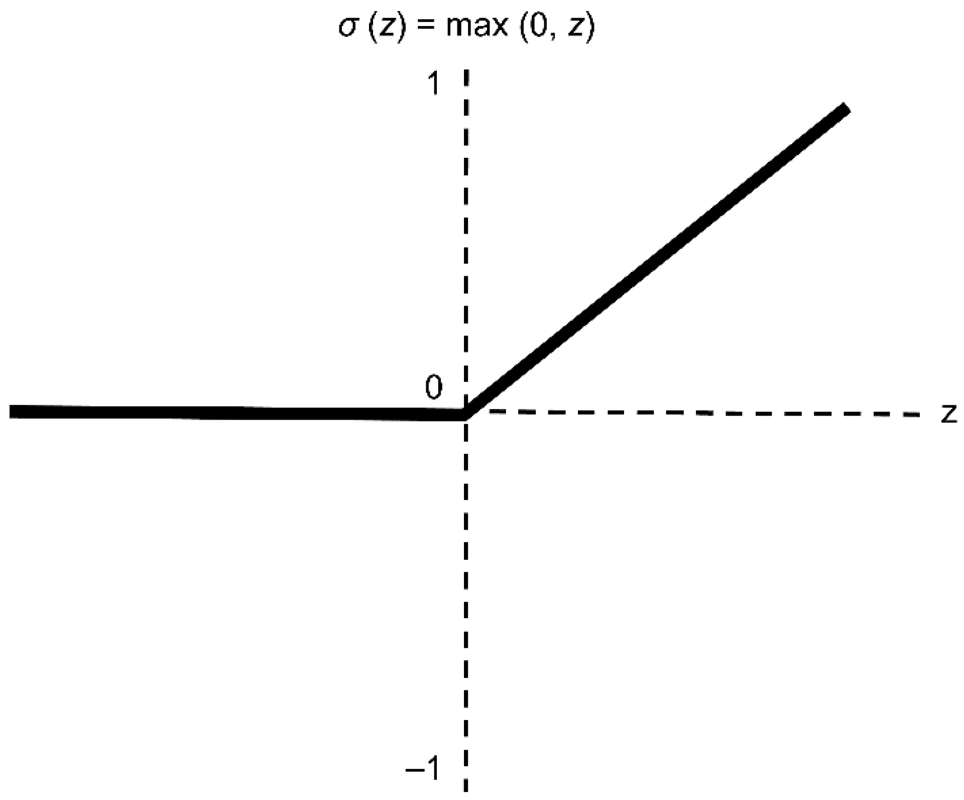
A critical benefit that has substantially improved the functionality of feedforward networks comes from replacing sigmoid hidden units with piecewise linear hidden units, e.g., rectified linear units (ReLU), which are the most common activation functions used in NNs [36]. Thus, in this study, we used the ReLU function, which is expressed as follows:
The ReLU activation is depicted in Figure 1. Here, when z is negative, the function is zero; otherwise, the function is z. Despite this, the function is said to be non-linear, as values less than zero, or negative values, always result in zero. From this property, the gradient remains intact because multiplying by 1 does not change the value. The diminishing error of the slope occurs when the activation function slope drops below the point where the NN cannot manage. Here, the ReLU slope is 0 when the input is less than 0 or a large value where the input is greater than 0. Thus, the ReLU is used to prevent a diminishing slope error as an effect of the activation function.
2.5. Cost Function
A cost function is considered the measure of the goodness of a Neural Network (NN) relative to the training sample and the predicted output. Weights and biases are dependent variables in the cost function implementation. It is a “one-value” that is used to rate the goodness of an NN’s overall performance. According to [37], ideally, a cost function will be reduced during training. The cost function can be expressed as follows:
The mean square error (MSE) is calculated by squaring the difference between each network output and its real label and averaging. Where E is our cost function (which is also referred to as loss function), N represents the number of training images, y is depicted as the true label (real), and a comprises a vector (such as network predictions). It is obvious to guess the importance of the cost function when considering its existence in the output layer and associating it with the adaptation of weight in the network. In addition, it is significant to modify the cost function within the output layer because it is constantly moving backward via the Net and does not change the equation of the hidden layer. Nevertheless, when used in the output layer, it should entirely be a differentiable unit to allow error derivatives computation for training [38].
2.6. ANN Implementation
In this study, Google Colab Notebook was used to write the code for the deck condition, superstructure, and substructure models using TensorFlow and Keras. One critical feature of Google Colab is that it offers an unlimited and open-source ecosystem, known as TensorFlow, that assists the development and unveiling of the platform in compliance with the Apache 2.0 license. In addition, Keras, which is an API for high-quality deep learning, realizes the easy establishment, training, evaluation, and testing of various NNs. Combined, Keras and TensorFlow form the tf.keras stack, where Keras serves as the backend to provide extra essential capabilities [39].
In this study, an NVIDIA Tesla P100-PCIE-16GB Graphics Processing Unit (GPU) was used in the training phase. Here, dropout, which is a simple method to prevent overfitting in NNs, was applied to realize to reduce computational costs and realize effective regularization in order to reduce overfitting while improving the generalization error [40]. The dropout rate was set to 0.25, and the Adam optimizer was applied with a learning rate of 0.0001. The Adam optimization algorithm refers to a stochastic gradient add-on that is frequently applied in deep learning approaches. The Adam optimization algorithm exploits the advantages of two state-of-the-art optimization methods, i.e., Adaptive Gradient Algorithm (AdaGrad), which handles sparse gradients, and Root Mean Square Propagation (RMSProp), which handles objectives that are considered to be nonstationary [41]. The error gradient estimate accuracy associated with the NN training process was regulated with a batch size of 64. A single cycle through the entire training dataset is referred to as an epoch. Typically, a few epochs are required to train an NN. Initially, the constructed NN comprises 200 epochs. The network was updated to determine the effect of increasing the number of epochs. Then, an analysis demonstrated that the training process where the epoch count for the three models—deck, superstructure, and substructure—read 700 epochs created the NN network with the best performance. Table 3 shows the model training characteristics for the deck, superstructure, and substructure models.
2.7. Feature Selection
The advantage of the approach used to select variables is that it ensures smooth implementation of the ANN model, i.e., only variables that affect the output are selected. In addition, the essential factors that determine the bridge condition rating were selected as the input variables. Statistical analyses performance regarding the correlations testing to ascertain the statistical relationship that occurs between the database parameters and the bridge condition ratings is observed. According to [42], if the correlation coefficient value is less than 0.3, it is considered to be statistically independent; thus, linear contribution does not exist with one another. However, due to the NN model’s ability to handle the complex relationships of various nonlinear parameters, it is unnecessary to apply typical statistical methods, which could result in poor detection of the underlying output–input relationships. Thus, more factors were selected, and their corresponding influences on the ANN models were evaluated equally.
As shown in Table 4, it is clear that the identified parameters regarding design load, type of support, type of design, deck structure type, and age complied with the deck rating statistics. In addition, the parameters regarding design load, type of support, year of construction, and age complied with the superstructure rating statistics. Finally, the parameters regarding the design load, type of design, type of support, year built, and age complied with the substructure rating statistics. The first ANN models were developed using the input parameters. Here, the effect of additional parameters on network performance was examined. Additional factors to aid in the examination consisted of parameters fetched from interrelation analyses whose locations were beyond the statistically dependent bandwidths. These parameters included ADT, number of spans, structure length, skew, type of service on, deck width, and material type. To examine the effect of these additional parameters on the ANN models, the models were trained using statistically verified parameters. Then, the performance of the baseline model and the newly trained network was compared. Here, variations occurring in the forecasting performance were determined to evaluate model performance.
The proposed initial models were validated using the baseline configurations for the deck, superstructure, and substructure models. Then, we evaluated the performance of the baseline models. The results demonstrated that the initial ANN models with the baseline model’s configuration were entirely ineffective in terms of predicting the deck, superstructure, and substructure conditions. Therefore, additional ANN models were developed using additional input parameters for the baseline models, and the architecture of the remaining models was maintained to determine the final input features.
In the case of the deck model, the following input parameters provided the best performance with the initial ANN models: year built, skew, ADT, design type, span number in the main unit, structure length, deck width, design load, type of support, deck type, and structure age. Similarly, in the case of superstructure and substructure models, the input parameters for optimal performance with initial ANN models included the year built, skew, ADT, design type, span number in the main unit, structure length, deck width, design load, type of support, material type, and structure age. The corresponding sizes of the feature matrices used to train and test the ANN models to predict the deck, superstructure, and substructure conditions were 68,652 × 11, 79,821 × 11, and 102,015 × 11, respectively.
2.8. Network Architecture
After selecting the input variable, we determined both the input size and output size. However, numerous dimensions of the network architecture are unknown. The network’s predictive performance is heavily influenced by its architecture; thus, it must be chosen and handled carefully. The additional architectural parameters include the number of hidden layers and the number of neurons in each hidden layer.
It is known that the architecture of an NN can influence network performance; however, to the best of our knowledge, there are no standard methods to evaluate optimal network architectures. As a result, in this study, different networks with various architectures were implemented to identify the best-performing NN. This evaluation was conducted after executing various systematic variations to identify the optimal number of hidden layers and the optimal number of neurons in each hidden layer.
Depending on the above assertions, training of the various NN architectures was performed, and they were verified depending on the dataset. This was conducted depending on the node number in all hidden layers and the total number of variants in the hidden layers. Here, the goal was to select the ANN model with the optimal architecture. First, a 32-neuron ANN model with a single hidden layer was subjected to the training and validation processes. Then, this model was modified to include two hidden layers with 16 and 32 neurons, respectively. In the subsequent configuration, the number of neurons in both hidden layers was increased by 32 and 256 neurons in each layer. Then, a third hidden layer was introduced, where the number of neurons in the first, second, and third hidden layers was 16, 32, and 64, respectively. In addition, the model with three hidden layers was subjected to training and validation, and the resulting number of neurons in the respective layers was 32, 256, and 512 neurons. Then, a configuration with four hidden layers was subjected to training and validation with 32, 256, 512, and 512 neurons, respectively. In the subsequent step, we attempted to evaluate the effect of varying the number of layers. Here, the total number of layers was increased to 5, 6, 7, 8, 9, and 14, where the combinations of neurons were 32, 256, 512, 512, and 512, respectively. All the models with hidden layer counts beyond four layers were subjected to training and validation using 512 neurons. The architectures of the different models and their respective validation are detailed in Table 5.
Next, the various networks affiliated with the deck, superstructure, and substructure models were trained and validated, where various nodes in the hidden layers were executed. Here, we found that the model with the smallest mean absolute error (MAE) and highest coefficient of determination (R2) was simulated to determine the verification set in order to identify which deck, superstructure, and substructure models demonstrated the best performance.
In this analysis, the MAE metric was used to determine the prediction accuracy of the models. Essentially, MAE represents the mean (average) deviation of the predicted values from observation values [43]. As shown in Table 5, the model with seven hidden layers obtained the smallest MAE value of 0.10 for the bridge deck model. In another case, the model with six hidden layers obtained MAE values of 0.10 and 0.11 for the bridge superstructure and substructure models, respectively. In addition, we found that there was a gradual reduction in the MAE values as the number of hidden layers increased from one to seven. For models with greater than seven hidden layers, we found that the MAE value began to increase again. Thus, we observed a tradeoff relationship between accuracy and the number of hidden layers. In addition, the results exhibited reduced accuracy when additional computations were performed.
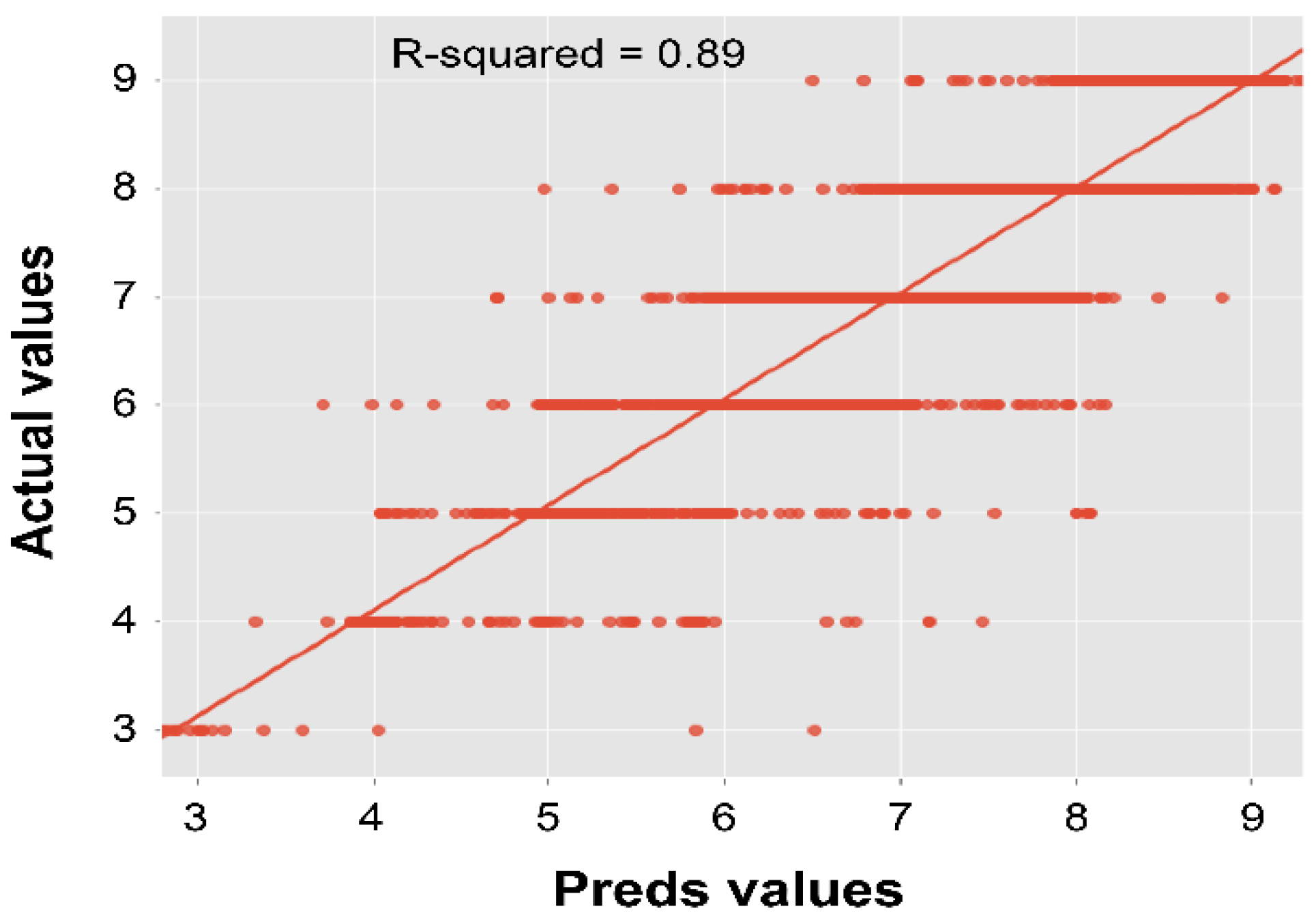
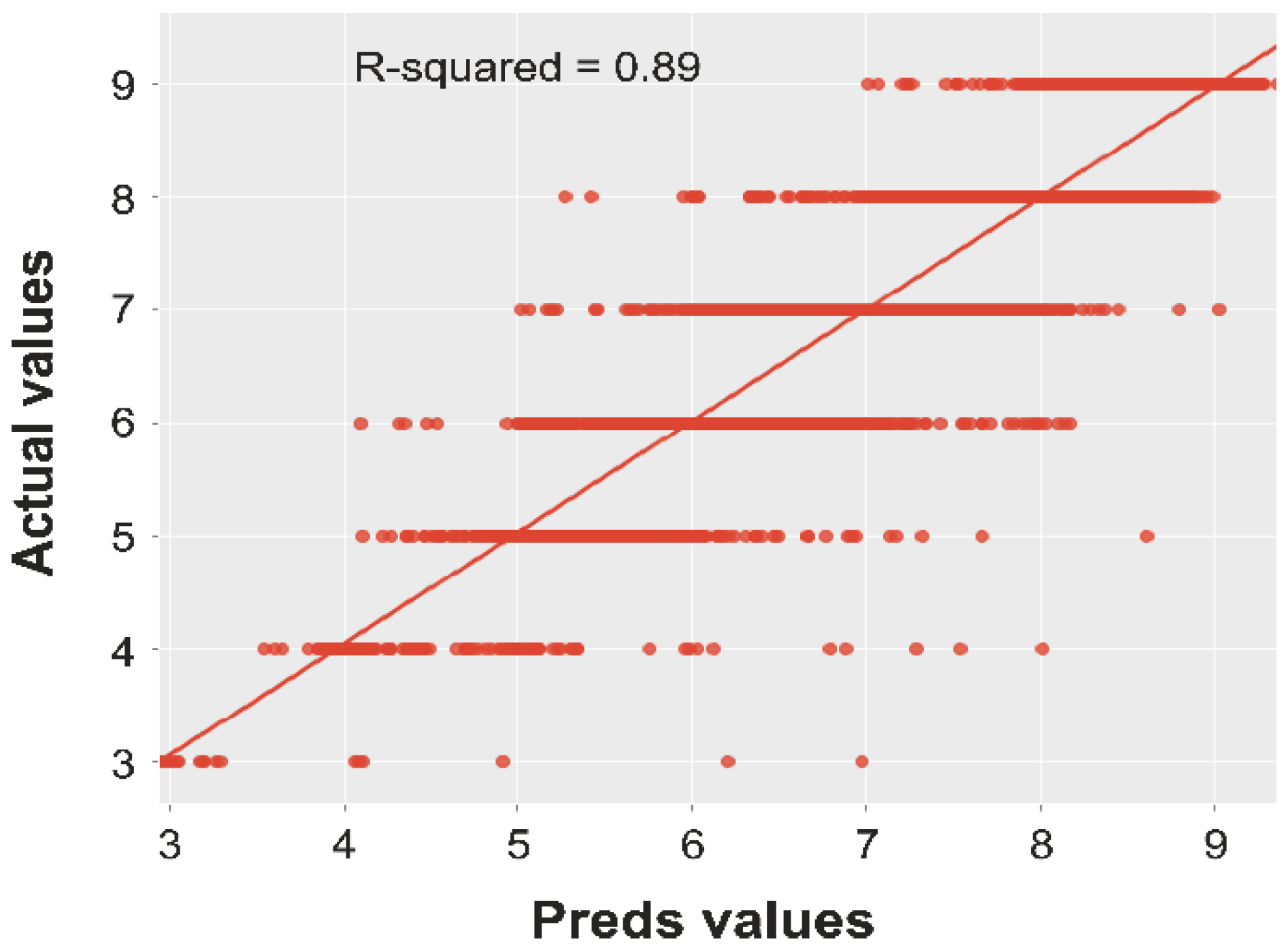
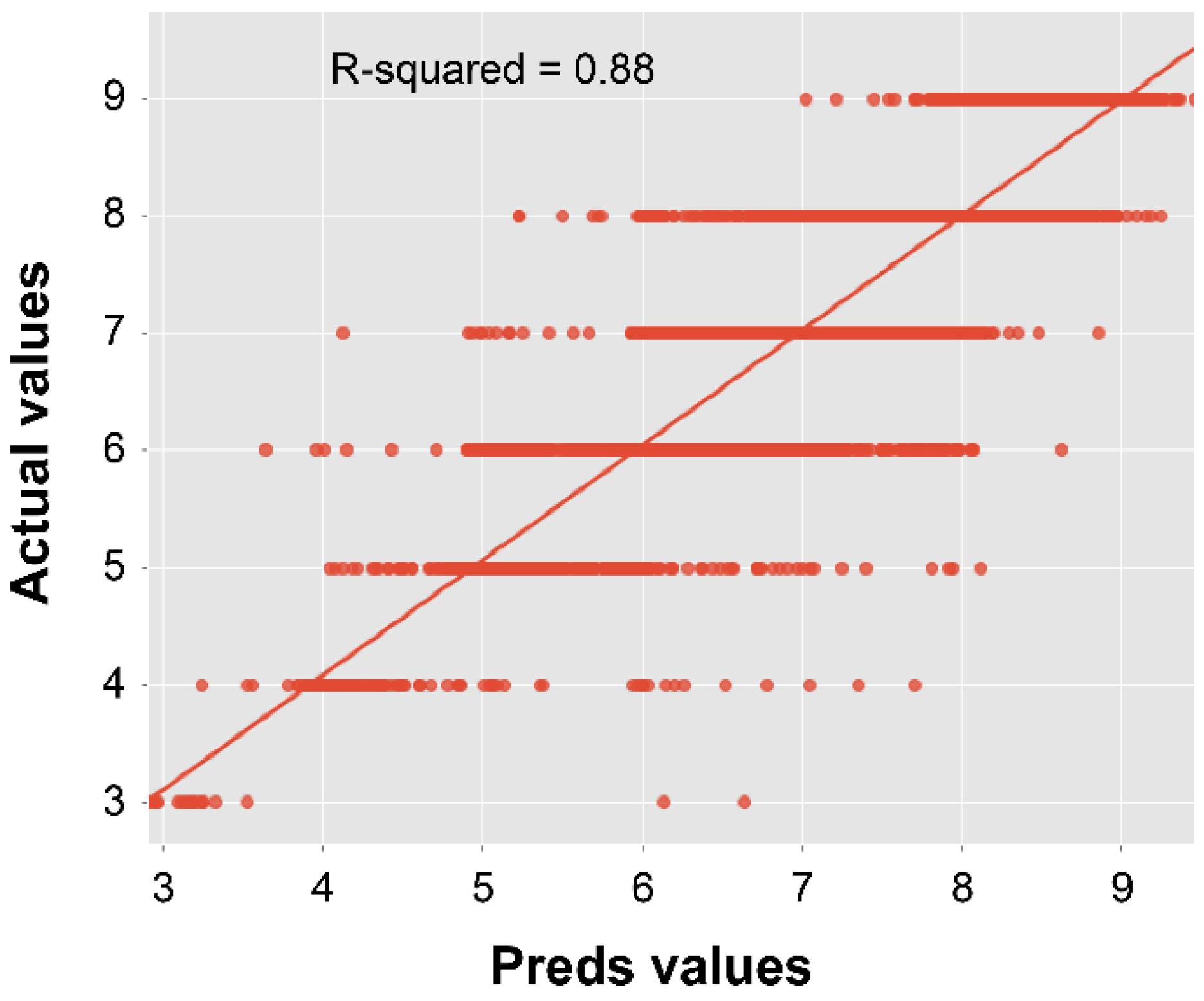
The second set of results is related to the coefficient of determination, i.e., the R2 value, which represents a comparison of the mutual relationship between the predicted and real values. Table 5 shows the R2 values obtained by the deck, superstructure, and substructure models with different architectures. Similar to the MAE analysis, the highest R2 value for the bridge deck model was obtained by the model with seven hidden layers (0.89), as shown in Figure 2. In addition, the highest R2 value for both the superstructure and substructure models was obtained by the models with six hidden layers (0.89 and 0.88, respectively), as shown in Figure 3 and Figure 4, respectively.
We found that the deck model with an input layer containing 11 neurons, seven hidden layers with 32, 256, 512, 512, 512, 512, and 512 neurons, respectively, and an output layer with one neuron and a linear activation function obtained the overall smallest MAE value and the highest R2 value. In addition, the superstructure and substructure models had an input layer containing 11 neurons, six hidden layers with 32, 256, 512, 512, 512, and 512 neurons, respectively, and an output layer with a single neuron and a linear activation function obtained the lowest MAE value and the highest R2 value.
3. Results and Discussion
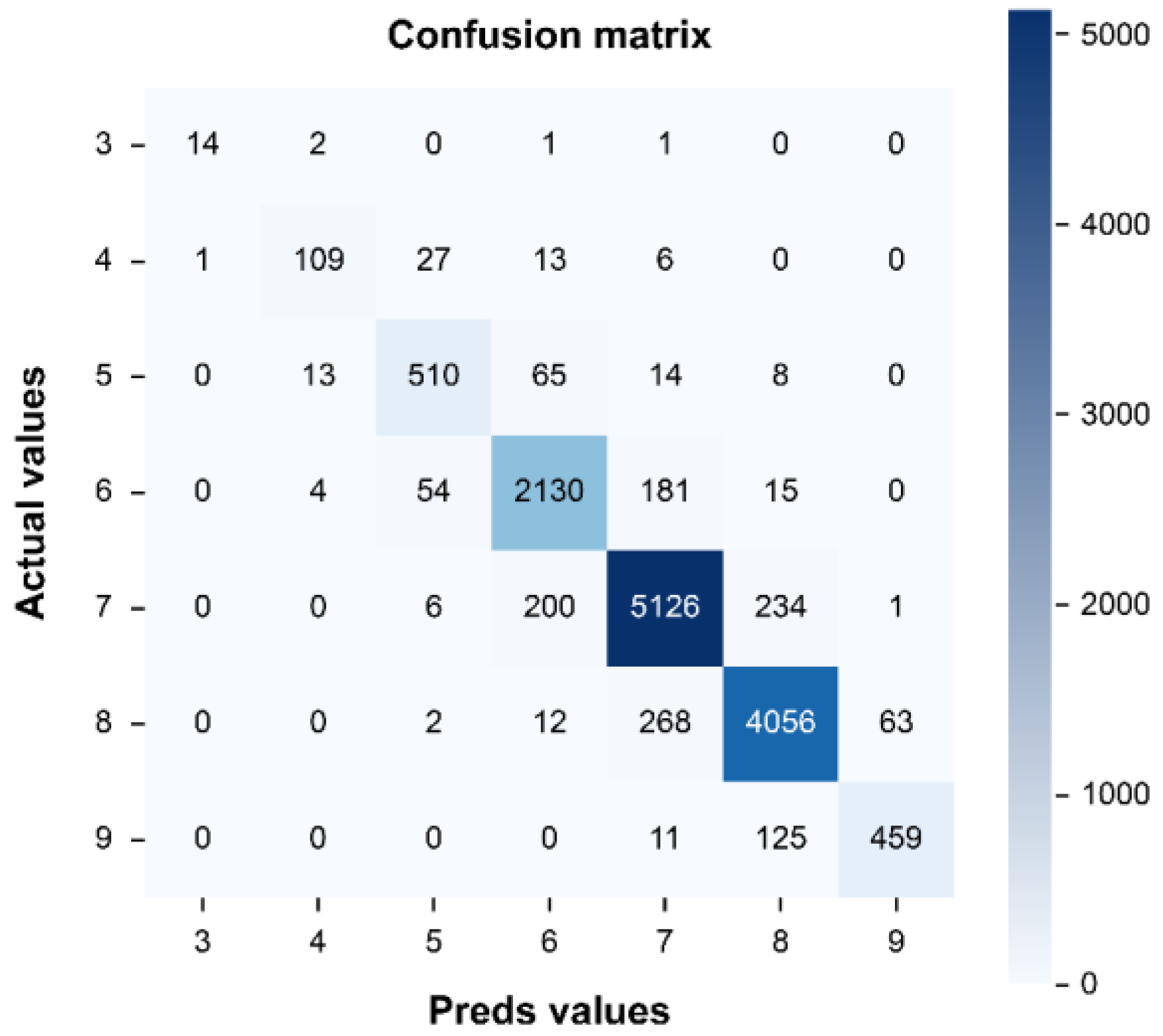
A confusion matrix was applied to evaluate the performance of the ANN models in terms of predicting the condition ratings of the different bridge components. Essentially, confusion matrices consist of tabular illustrations of MLP predicting capability [44]. The target outputs were compared, and the results were tabulated against the network’s predicted rating. Confusion matrices were developed in order to facilitate testing of the data sets. Here, 20% of the data was selected to test the models.
Here, the computation of functionality variables for algorithms was performed by evaluating the true positive (TP), false positive (FP), true negative (TN), and false negative (FN) values all as found in the confusion matrix. In addition, accuracy, effectiveness, recall, the F1-score, and the macroaverage [45] were investigated.
When performing macroaveraging, the measure is initially computed per label, and an average is taken according to the total number of labels. Through microaveraging, the equal weight of each label is identified, regardless of the given label’s appearance frequency.
where and are derived as the arithmetic mean of the accuracy and recall scores for each class and represents an individual class of each matrix.
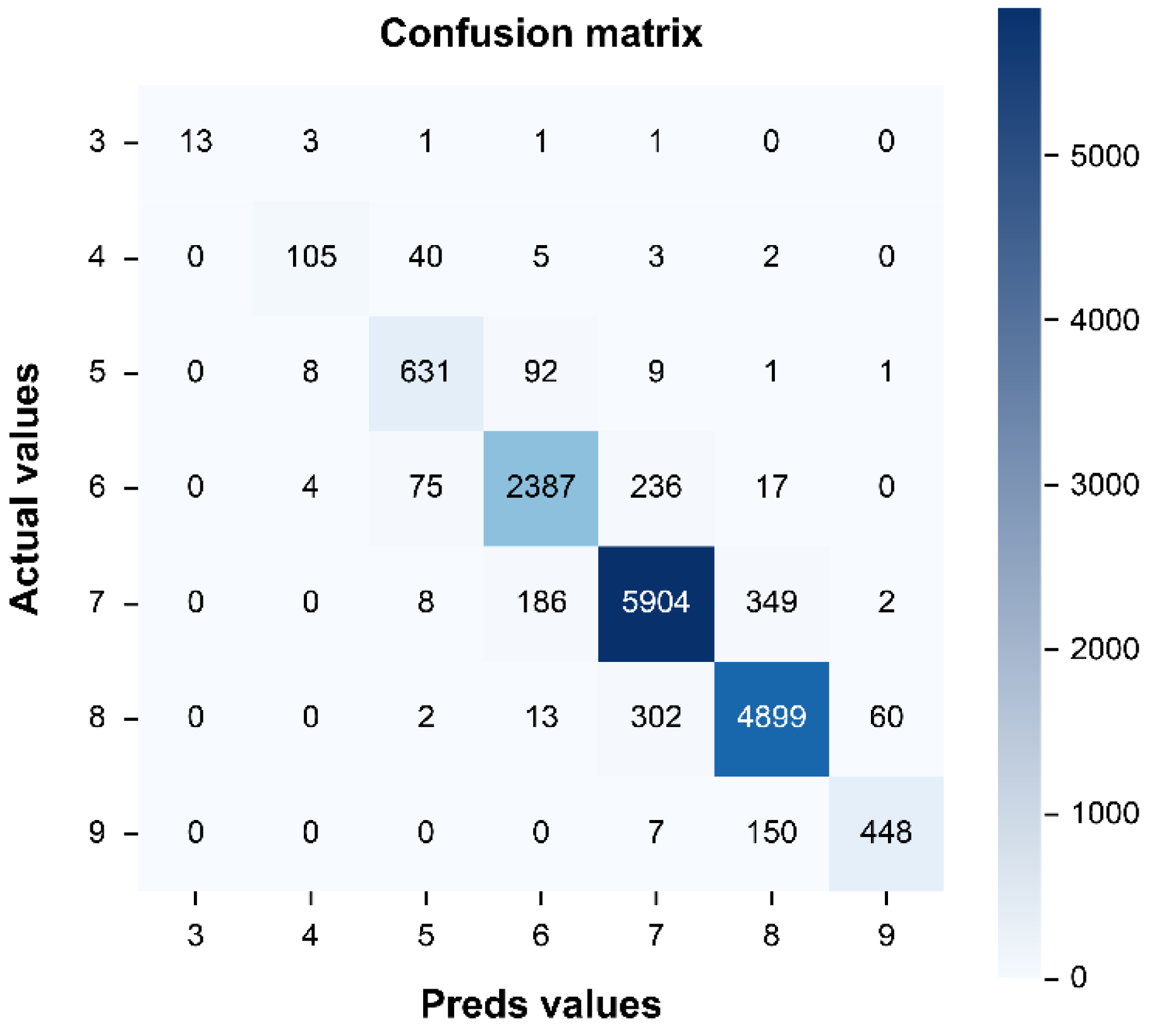
Figure 5, Figure 6 and Figure 7 show the confusion matrices for the bridge deck, superstructure, and substructure condition models. To compute for parameters like TP, TN, FN, and FP, we must first determine their individual condition values. By definition, the TP value represents the number of correct predicted values, i.e., the values lying in the diagonal of the confusion matrix. The FN value represents the total number of values that lie in the corresponding row, excluding the TP. The FP value represents the total number of values in the corresponding column, excluding the TP. Finally, the TN of a given class represents the total number of columns and rows, where the respective column and row to these classes are excluded.
As shown in Figure 5, the TP, TN, FP, and FN values were 12,404, 81,059, 1327, and 1327, respectively, for the deck model. Similarly, Figure 6 shows that the TP, TN, FP, and FN values were 14,387, 94,212, 1578, and 1578, respectively, for the superstructure model. Finally, Figure 7 shows that the TP, TN, FN, and FP values were 18,198, 120, 213, 2205, and 2205, respectively, for the substructure model.
Condition model performance:
Deck accuracy = 12404/13729 = 0.90
Precision = 12404/(12404 + 1327) = 0.90
Recall = 12404/(12404 + 1327) = 0.90
F1-score = 2 × (0.9 × 0.9)/(0.9 + 0.9) = 0.90
Precision_(macroaverage) = (0.93 + 0.85 + 0.85 + 0.88 + 0.91 + 0.91 + 0.88)/7 = 0.89
Recall _(macroaverage) = (0.78 + 0.70 + 0.84 + 0.89 + 0.92 + 0.92)/7 = 0.83
F1-score _(macroaverage) = (0.85 + 0.77 + 0.84 + 0.89 + 0.92 + 0.92 + 0.82)/7 = 0.86
Similarly, for superstructure and substructure condition model performance measures:
Superstructure Accuracy = 14389/15965 = 0.90
Substructure Accuracy = 18198/20403 = 0.89
Table 6, Table 7 and Table 8 show the accuracy results obtained by the deck, superstructure, and substructure models. Equation 7 depicts the precision by providing an approximation of the accuracy associated with the model out of the summation of the predicted positive observations. This is a reasonable method to evaluate the conditions when FPs might have high costs. For example, the deck model obtained a precision value of 89%, which implies that there is an 11% probability that this model will predict an FP condition by incorrectly predicting some issue. Overall, the precision values of the three models were significantly high. Recall evaluates the summation of TPs estimated by the model. Here, all three models obtained recall values that were greater than 81%, which implies that if a particular section of the bridge is characterized by repair issues (TP) and the corresponding model falsely predicts this (FN), then the bridge may suffer some damage conditions, particularly where the issue can affect other sections of the bridge.
Overall, the F1-score of all three bridge component models was greater than 85%, which means that the number of FPs and FNs was low. In addition, it signifies that the model has predicted both correct and incorrect predictions. From these results, we conclude that both the recall and precision of the models are significantly high. Nevertheless, it is still 12% probable that these models will predict incorrect results for the three bridge components. For example, a deck component parameter may yield an undue maintenance notification at a 14% probability.
Finally, the model obtained the highest accuracy (90%) for both the deck and superstructure components, and the model obtained 89% accuracy for the substructure component. These results imply that training was performed accurately with an error rate of approximately 10%. Here, accuracy was calculated using Equation (5), and it is significant regarding true positives or true negatives against the overall results. This implies that higher accuracy values significantly assist in the exploration of the number of data points rightly predicted when compared with the overall data points. As shown in Table 6, Table 7 and Table 8, the accuracy of the model was substantively high, and, in most cases, this model accurately predicted the outcomes of both TPs and TNs.
In this study, a confusion matrix was applied when measuring the performance of various elements, e.g., the deck, superstructure, and substructure conditions. Ideally, the testing set was used to formulate the confusion matrices, which provided the generalizability of the network to unseen information. We found that the deck, superstructure, and substructure models obtained accuracy that was greater than 89% on the test data.
The input variables are ranked based on a set of criteria, such as the ratio of error with omission to baseline error, and this is completed depending on the magnitude. According to the findings, the age and type of support have a high impact on the deck condition. In addition, the age and type of design have a high impact on the condition of the superstructure. Age and year built have great effects on the condition of the substructure, whereas the average daily traffic has the least impact on bridge condition.
4. Conclusions
ANN modeling techniques in AI can incorporate multiple parameters into a model that is both sophisticated and nonlinear. In terms of bridge engineering, an ANN model can be trained and tested on data available in the NBI database in order to predict the deterioration of a bridge.
In this study, various ANN models with different configurations were utilized and formulated to perform predictions about the deterioration of bridge deck, superstructure, and substructure components. The proposed model considers a comprehensive set of geometric and functional parameters of the bridge structure to enhance prediction accuracy. In addition, many standardized approaches are adopted in the proposed model to improve its performance, including the evaluation of the most optimal set of model inputs, preprocessing and dividing the data, selecting internal parameters for control optimization, and model validation. During the data preprocessing stage, unnecessary and complicated NBI data were cleaned so that appropriate and unbiased data were input to the model. Then, the input data and results are normalized in order to conveniently train and test on this dataset and produce standardized results. Then, the finalized dataset is utilized to identify the most appropriate ANN architecture to obtain optimal accuracy for a given number of hidden layers and neurons. Finally, with the optimal ANN configuration, the proposed model is trained and tested for various components (i.e., the bridge deck, superstructure, and substructure components) for the dataset. The results were then evaluated in terms of accuracy, precision, recall, and F1-score. Overall, the accuracy of the final model trained for the deck, substructure, and superstructure components was found to be greater than 89% on the NBI dataset. Similarly, the F1-score, recall, and precision values were all greater than 81%. Therefore, we consider that the proposed ANN models have allowed us to identify a strong correlation between the predicted values and actual values in the NBI dataset.
Finally, the proposed ANN models were used to develop a bridge deterioration model to predict deterioration in all bridge systems. Consequently, this model is perceived to assist in furnishing an ideal plan for bridge maintenance, scheduling any bridge with an imminent requirement to earmark appropriate funds for its maintenance and repair.
However, the performance of the proposed ANN models can be improved. For example, the model’s accuracy is dependent on a number of factors such as excessive training on larger and more diverse datasets and configurations of ANN models; therefore, the proposed model can be improved by considering the most optimal combination of these factors.
Author Contributions
Conceptualization, E.A. and E.C.; methodology, E.A.; software, E.A.; validation, E.A.; formal analysis, E.A.; investigation, E.A.; resources, E.A.; data curation, E.A.; writing—original draft preparation, E.A.; writing—review and editing, E.C.; visualization, E.A.; supervision, E.C.; project administration, E.C. All authors have read and agreed to the published version of the manuscript.
Funding
This research received no external funding.
Institutional Review Board Statement
Not applicable.
Informed Consent Statement
Not applicable.
Data Availability Statement
Readers interested in the data presented in this study are encouraged to contact the corresponding author.
Acknowledgments
The authors wish to thank the Faculty of Civil and Environmental Engineering at the University of Toledo for their support.
Conflicts of Interest
The authors declare no conflict of interest.
References
- American Society of Civil Engineers (ASCE). Infrastructure Report Card: A Comprehensive Assessment of America’s Infrastructure; ASCE: Reston, VA, USA, 2017. [Google Scholar]
- Madanat, S.; Mishalani, R.; Ibrahim, W.H.W. Estimation of infrastructure transition probabilities from condition rating data. J. Infrastruct. Syst. 1995, 1, 120–125. [Google Scholar] [CrossRef]
- Thompson, P.D.; Small, E.P.; Johnson, M.; Marshall, A.R. The Pontis bridge management system. Struct. Eng. Int. 1998, 8, 303–308. [Google Scholar] [CrossRef]
- Thompson, P.D. Decision Support Analysis in Ontario’s New Bridge Management System. In Structures 2001: A Structural Engineering Odyssey; ASCE: Reston, VA, USA, 2001; pp. 1–2. [Google Scholar] [CrossRef]
- Urs, N.; Manthesh, B.S.; Jayaram, H.; Hegde, M.N. Residual life assessment of concrete structures-a review. Int. J. Eng. Tech. Res. 2015, 3, iss3. [Google Scholar]
- Kayser, J.R.; Nowak, A.S. Reliability of corroded steel girder bridges. Struct. Saf. 1989, 6, 53–63. [Google Scholar] [CrossRef] [Green Version]
- Adams, T.M.; Sianipar, P.R.M. Project and network level bridge management. In Transportation Congress, Volumes 1 and 2: Civil Engineers—Key to the World’s Infrastructure; ASCE: Reston, VA, USA, 1995; pp. 1670–1681. [Google Scholar]
- Morcous, G.; Rivard, H.; Hanna, A.M. Modeling bridge deterioration using case-based reasoning. J. Infrastruct. Syst. 2002, 8, 86–95. [Google Scholar] [CrossRef]
- Sanders, D.H.; Zhang, Y.J. Bridge deterioration models for states with small bridge inventories. Transp. Res. Rec. 1994, 1442, 101–109. [Google Scholar]
- Jiang, Y.; Saito, M.; Sinha, K.C. Bridge Performance Prediction Model Using the Markov Chain, no. 1180; NASEM: Washington, DC, USA, 1988. [Google Scholar]
- Tolliver, D.; Lu, P. Analysis of bridge deterioration rates: A case study of the northern plains region. J. Transp. Res. Forum. 2012, 50. [Google Scholar] [CrossRef]
- Chase, S.B.; Small, E.P.; Nutakor, C. An in-depth analysis of the national bridge inventory database utilizing data mining, GIS and advanced statistical methods. Transp. Res. Circ. 1999, 498, 1–17. [Google Scholar]
- Morcous, G.; Lounis, Z.; Mirza, M.S. Identification of environmental categories for Markovian deterioration models of bridge decks. J. Bridg. Eng. 2003, 8, 353–361. [Google Scholar] [CrossRef]
- Abdelkader, E.M.; Zayed, T.; Marzouk, M. A computerized hybrid Bayesian-based approach for modelling the deterioration of concrete bridge decks. Struct. Infrastruct. Eng. 2019, 15, 1178–1199. [Google Scholar] [CrossRef]
- Jiang, Y.; Sinha, K.C. Bridge service life prediction model using the Markov chain. Transp. Res. Rec. 1989, 1223, 24–30. [Google Scholar]
- Lee, Y.; Chang, L.M. Econometric model for predicting deterioration of bridge deck expansion joints. Transp. Res. Circ. No. E-C049 2003, No.E-C049, 255–265. [Google Scholar]
- Madanat, S.M.; Karlaftis, M.G.; McCarthy, P.S. Probabilistic infrastructure deterioration models with panel data. J. Infrastruct. Syst. 1997, 3, 4–9. [Google Scholar] [CrossRef]
- Kong, J.S.; Frangopol, D.M. Life-cycle reliability-based maintenance cost optimization of deteriorating structures with emphasis on bridges. J. Struct. Eng. 2003, 129, 818–828. [Google Scholar] [CrossRef]
- Saydam, D.; Bocchini, P.; Frangopol, D.M. Time-dependent risk associated with deterioration of highway bridge networks. Eng. Struct. 2013, 54, 221–233. [Google Scholar] [CrossRef]
- Frangopol, D.M.; Bocchini, P. Bridge network performance, maintenance and optimisation under uncertainty: Accomplishments and challenges. Struct. Infrastruct. Eng. 2012, 8, 341–356. [Google Scholar] [CrossRef]
- Liu, H.; Zhang, Y. Bridge condition rating data modeling using deep learning algorithm. Struct. Infrastruct. Eng. 2020, 16, 1447–1460. [Google Scholar] [CrossRef]
- Mukherjee, A.; Deshpande, J.M.; Anmala, J. Prediction of buckling load of columns using artificial neural networks. J. Struct. Eng. 1996, 122, 1385–1387. [Google Scholar] [CrossRef]
- Hung, S.-L.; Kao, C.Y.; Lee, J.C. Active pulse structural control using artificial neural networks. J. Eng. Mech. 2000, 126, 839–849. [Google Scholar] [CrossRef] [Green Version]
- Tohidi, S.; Sharifi, Y. Load-carrying capacity of locally corroded steel plate girder ends using artificial neural network. Thin-Walled Struct. 2016, 100, 48–61. [Google Scholar] [CrossRef]
- Okazaki, Y.; Okazaki, S.; Asamoto, S.; Chun, P. Applicability of machine learning to a crack model in concrete bridges. Comput. Civ. Infrastruct. Eng. 2020, 35, 775–792. [Google Scholar] [CrossRef]
- Wang, J.; Xue, S.; Xu, G. A Hybrid Surrogate Model for the Prediction of Solitary Wave Forces on the Coastal Bridge Decks. Infrastructures 2021, 6, 170. [Google Scholar] [CrossRef]
- Dechkamfoo, C.; Sitthikankun, S.; Na Ayutthaya, T.K.; Manokeaw, S.; Timprae, W.; Tepweerakun, S.; Tengtrairat, N.; Aryupong, C.; Jitsangiam, P.; Rinchumphu, D. Impact of Rainfall-Induced Landslide Susceptibility Risk on Mountain Roadside in Northern Thailand. Infrastructures. 2022, 7, 17. [Google Scholar] [CrossRef]
- Sobanjo, J.O. A neural network approach to modeling bridge deterioration. Comput. Civ. Eng. 1997, 11, 623–626. [Google Scholar]
- Huang, Y.-H. Artificial neural network model of bridge deterioration. J. Perform. Constr. Facil. 2010, 24, 597–602. [Google Scholar] [CrossRef]
- Xu, G.; Chen, Q.; Chen, J. Prediction of solitary wave forces on coastal bridge decks using artificial neural networks. J. Bridg. Eng. 2018, 23, 4018023. [Google Scholar] [CrossRef]
- Weinstein, J.C.; Sanayei, M.; Brenner, B.R. Bridge damage identification using artificial neural networks. J. Bridg. Eng. 2018, 23, 4018084. [Google Scholar] [CrossRef] [Green Version]
- Cho, Y.K.; Leite, F.; Behzadan, A.; Wang, C. Computing in Civil Engineering 2019: Smart Cities, Sustainability, and Resilience; ASCE: Reston, VA, USA, 2019. [Google Scholar]
- Fabianowski, D.; Jakiel, P.; Stemplewski, S. Development of artificial neural network for condition assessment of bridges based on hybrid decision making method–Feasibility study. Expert Syst. Appl. 2021, 168, 114271. [Google Scholar] [CrossRef]
- Srinivasan, D.; Liew, A.C.; Chang, C.S. A neural network short-term load forecaster. Electr. Power Syst. Res. 1994, 28, 227–234. [Google Scholar] [CrossRef]
- Mahmoud, O.; Anwar, F.; Salami, M.-J.E. Learning Algorithm Effect on Multilayer Feed forward Artificial Neural Network Performance in Image Coding. JESTEC: Subang Jaya, Selangor, Malaysia, 2007. [Google Scholar]
- Goodfellow, I.; Bengio, Y.; Courville, A. Deep Learning; MIT Press: Cambridge, MA, USA, 2016. [Google Scholar]
- Zhang, G.; Patuwo, B.E.; Hu, M.Y. Forecasting with artificial neural networks:: The state of the art. Int. J. Forecast. 1998, 14, 35–62. [Google Scholar] [CrossRef]
- Crone, S.F. Training artificial neural networks for time series prediction using asymmetric cost functions. In Proceedings of the 9th International Conference on Neural Information Processing, Yishun, Singapore, 18–22 November 2002; pp. 2374–2380. [Google Scholar] [CrossRef]
- Géron, A. Hands-on Machine Learning with Scikit-Learn, Keras, and TensorFlow: Concepts, Tools, and Techniques to Build Intelligent Systems; O’Reilly Media, Inc.: Sebastopol, CA, USA, 2019. [Google Scholar]
- Srivastava, N.; Hinton, G.; Krizhevsky, A.; Sutskever, I.; Salakhutdinov, R. Dropout: A simple way to prevent neural networks from overfitting. J. Mach. Learn. Res. 2014, 15, 1929–1958. [Google Scholar]
- Kingma, D.P.; Ba, J. Adam: A method for stochastic optimization. arXiv 2014, arXiv:1412.6980. [Google Scholar]
- Ayyub, B.M.; McCuen, R.H. Probability, Statistics, and Reliability for Engineers and Scientists. Technometrics 2003, 45, 276. [Google Scholar] [CrossRef]
- Wang, H.; Zhang, Y.-M.; Mao, J.-X. Sparse Gaussian process regression for multi-step ahead forecasting of wind gusts combining numerical weather predictions and on-site measurements. J. Wind Eng. Ind. Aerodyn. 2022, 220, 104873. [Google Scholar] [CrossRef]
- Kohavi, R. Special Issue on Applications of Machine Learning and the Knowledge Discovery Process; Kluwer: Alphen aan den Rijn, The Netherlands, 1998. [Google Scholar]
- Wang, F.; Song, G.; Mo, Y. Shear loading detection of through bolts in bridge structures using a percussion-based one-dimensional memory-augmented convolutional neural network. Comput. Civ. Infrastruct. Eng. 2021, 36, 289–301. [Google Scholar] [CrossRef]
Figure 1.
ReLU activation function.

Figure 2.
Test coefficient of the determination analysis for the deck condition model.

Figure 3.
Test coefficient of the determination analysis for the superstructure condition model.

Figure 4.
Test coefficient of the determination analysis for the substructure condition model.

Figure 5.
Deck confusion matrix result for the test data.

Figure 6.
Superstructure confusion matrix result for the test data.

Figure 7.
Substructure confusion matrix result for the test data.


Table 1.
FHWA ratings for bridge conditions (FHWA, 1995).
| Code | Description |
|---|---|
| 9 | Excellent condition |
| 8 | Very good condition (no problems noted) |
| 7 | Good condition (some minor problems) |
| 6 | Satisfactory condition (structural elements show some minor deterioration) |
| 5 | Fair condition (all primary structural elements are sound but may have minor section loss, cracking, spalling, or scour) |
| 4 | Poor condition (advanced section loss, deterioration, spalling, or scour) |
| 3 | Serious condition (loss of section, deterioration, spalling, or scour have seriously affected primary structural components; local failures are possible, and fatigue cracks in steel or shear cracks in concrete may be present) |
| 2 | Critical condition (advanced deterioration of primary structural elements. Fatigue cracks in steel or shear cracks in concrete may be present or scour may have removed substructure support. Unless closely monitored, it may be necessary to close the bridge until corrective action is taken.) |
| 1 | Imminent failure condition (major deterioration or section loss present in critical structural components or obvious vertical or horizontal movement affecting structure stability; bridge is closed to traffic, but corrective action may permit light service) |
| 0 | Failed condition (out of service; beyond corrective action) |
Table 2.
Description of FHWA items.
| Data Item | Item | |
|---|---|---|
| Inventory | Highway agency district | FHWA 2 |
| Year built | FHWA 27 | |
| Average daily traffic (ADT) | FHWA 29 | |
| Design load | FHWA 31 | |
| Skew | FHWA 34 | |
| Material type | FHWA 43A | |
| Structure type | FHWA 43B | |
| Number of main spans | FHWA 45 | |
| Structure length | FHWA 49 | |
| Deck width | FHWA 52 | |
| Year reconstructed | FHWA106 | |
| Deck structure type | FHWA 107 | |
| Rating | Deck condition | FHWA 58 |
| Superstructure condition | FHWA 59 | |
| Substructure condition | FHWA 60 |
Table 3.
Model training parameters.
| Parameter | Implementation |
|---|---|
| Dropout | 0.25 |
| Epochs | 700 |
| Activation function | ReLU |
| Optimization function | Adam |
Table 4.
Correlation coefficient results.
| Parameters | Deck | Superstructure | Substructure |
|---|---|---|---|
| Condition | Condition | Condition | |
| Highway district | −0.04 | −0.08 | −0.09 |
| Year built | 0.19 | 0.41 | 0.33 |
| Average daily traffic (ADT) | −0.06 | −0.03 | −0.09 |
| Design load | 0.42 | 0.32 | 0.35 |
| Skew | −0.04 | −0.03 | −0.02 |
| Type of service on | −0.09 | −0.04 | −0.1 |
| Type of service under | 0.13 | 0.02 | 0.07 |
| Material type | −0.07 | 0.03 | 0.04 |
| Design type | 0.34 | 0.19 | 0.3 |
| Type of support | −0.31 | −0.34 | −0.2 |
| Number of spans in main unit | −0.19 | −0.05 | −0.14 |
| Length of maximum span | −0.03 | 0.02 | 0.04 |
| Structure length | −0.13 | 0.02 | −0.07 |
| Deck width | −0.12 | 0.021 | 0.19 |
| Deck structure type | 0.36 | 0.03 | 0.02 |
| Age | −0.49 | −0.48 | −0.61 |
Table 5.
Validation of the numerous network architectures.
| Model Architecture | Deck | Superstructure | Substructure | |||
|---|---|---|---|---|---|---|
| MAE | R2 | MAE | R2 | MAE | R2 | |
| 11-32-1 | 0.49 | 0.41 | 0.52 | 0.36 | 0.46 | 0.46 |
| 11-16-32-1 | 0.47 | 0.43 | 0.51 | 0.38 | 0.45 | 0.47 |
| 11-32-256-1 | 0.42 | 0.55 | 0.45 | 0.48 | 0.41 | 0.54 |
| 11-16-32-64-1 | 0.45 | 0.48 | 0.48 | 0.42 | 0.44 | 0.49 |
| 11-32-256-512-1 | 0.3 | 0.66 | 0.25 | 0.73 | 0.27 | 0.7 |
| 11-32-256-512-512-1 | 0.22 | 0.75 | 0.2 | 0.78 | 0.24 | 0.73 |
| 11-32-256-512-512-512-1 | 0.15 | 0.83 | 0.16 | 0.82 | 0.15 | 0.82 |
| 11-32-256-512-512-512-512-1 | 0.11 | 0.88 | 0.1 | 0.89 | 0.11 | 0.88 |
| 11-32-256-512-512-512-512-512-1 | 0.1 | 0.89 | 0.11 | 0.88 | 0.12 | 0.87 |
| 11-32-256-512-512-512-512-512-512-1 | 0.12 | 0.86 | 0.12 | 0.86 | 0.13 | 0.86 |
| 11-32-256-512-512-512-512-512-512-512-1 | 0.14 | 0.83 | 0.14 | 0.83 | 0.14 | 0.84 |
| 11-32-256-512-512-512-512-512-512-512-512-512-512-512-512-1 | 0.16 | 0.81 | 0.17 | 0.81 | 0.21 | 0.76 |
Table 6.
Test accuracy of the deck model.
| Condition | Precision | Recall | F1-Score | Support |
|---|---|---|---|---|
| 3 | 0.93 | 0.78 | 0.85 | 18 |
| 4 | 0.85 | 0.7 | 0.77 | 156 |
| 5 | 0.85 | 0.84 | 0.84 | 610 |
| 6 | 0.88 | 0.89 | 0.89 | 2384 |
| 7 | 0.91 | 0.92 | 0.92 | 5567 |
| 8 | 0.91 | 0.92 | 0.92 | 4401 |
| 9 | 0.88 | 0.77 | 0.82 | 595 |
| accuracy | 0.9 | 13,731 | ||
| macro avg | 0.89 | 0.83 | 0.86 | 13,731 |
| weighted avg | 0.9 | 0.9 | 0.9 | 13,731 |
Table 7.
Test accuracy of the superstructure model.
| Condition | Precision | Recall | F1-Score | Support |
|---|---|---|---|---|
| 3 | 1 | 0.68 | 0.81 | 19 |
| 4 | 0.88 | 0.68 | 0.76 | 155 |
| 5 | 0.83 | 0.85 | 0.84 | 742 |
| 6 | 0.89 | 0.88 | 0.88 | 2719 |
| 7 | 0.91 | 0.92 | 0.91 | 6449 |
| 8 | 0.9 | 0.93 | 0.92 | 5276 |
| 9 | 0.88 | 0.74 | 0.8 | 605 |
| accuracy | 0.9 | 15,965 | ||
| macro avg | 0.9 | 0.81 | 0.85 | 15,965 |
| weighted avg | 0.9 | 0.9 | 0.9 | 15,965 |
Table 8.
Test accuracy of the substructure model.
| Condition | Precision | Recall | F1-Score | Support |
|---|---|---|---|---|
| 3 | 0.94 | 0.84 | 0.89 | 19 |
| 4 | 0.85 | 0.78 | 0.81 | 154 |
| 5 | 0.85 | 0.77 | 0.81 | 671 |
| 6 | 0.88 | 0.89 | 0.89 | 4001 |
| 7 | 0.89 | 0.91 | 0.9 | 7752 |
| 8 | 0.91 | 0.91 | 0.91 | 6876 |
| 9 | 0.88 | 0.75 | 0.81 | 930 |
| accuracy | 0.89 | 20,403 | ||
| macro avg | 0.88 | 0.84 | 0.86 | 20,403 |
| weighted avg | 0.89 | 0.89 | 0.89 | 20,403 |
Publisher’s Note: MDPI stays neutral with regard to jurisdictional claims in published maps and institutional affiliations. |
© 2022 by the authors. Licensee MDPI, Basel, Switzerland. This article is an open access article distributed under the terms and conditions of the Creative Commons Attribution (CC BY) license (https://creativecommons.org/licenses/by/4.0/).
Share and Cite
MDPI and ACS Style
Althaqafi, E.; Chou, E. Developing Bridge Deterioration Models Using an Artificial Neural Network. Infrastructures 2022, 7, 101. https://doi.org/10.3390/infrastructures7080101
AMA Style
Althaqafi E, Chou E. Developing Bridge Deterioration Models Using an Artificial Neural Network. Infrastructures. 2022; 7(8):101. https://doi.org/10.3390/infrastructures7080101
Chicago/Turabian StyleAlthaqafi, Essam, and Eddie Chou. 2022. "Developing Bridge Deterioration Models Using an Artificial Neural Network" Infrastructures 7, no. 8: 101. https://doi.org/10.3390/infrastructures7080101