Article

Vision-Based Structural Monitoring: Application to a Medium-Span Post-Tensioned Concrete Bridge under Vehicular Traffic

School of Architecture and Design, University of Camerino, Viale della Rimembranza 3, 63100 Ascoli Piceno, Italy
*
Author to whom correspondence should be addressed.
Infrastructures 2023, 8(10), 152; https://doi.org/10.3390/infrastructures8100152
Submission received: 27 September 2023 / Revised: 16 October 2023 / Accepted: 16 October 2023 / Published: 17 October 2023

Abstract

:
Video processing for structural monitoring has attracted much attention in recent years thanks to the possibility of measuring displacement time histories in the absence of stationary points close to the structure, using hardware that is simple to operate and with accessible costs. Experimental studies show a unanimous consensus on the potentialities of vision-based monitoring to provide accurate results that can be equivalent to those obtained from accelerometers and displacement transducers. However, past studies mostly involved steel bridges and footbridges while very few applications can be found for concrete bridges, characterised by a stiffer response with lower displacement magnitudes and different frequency contents of their dynamic behaviour. Accordingly, the attention of this experimental study is focused on the application of a vision-based structural monitoring system to a medium-span, post-tensioned, simply supported concrete bridge, a very common typology in many road networks. The objective is to provide evidence on the quality of the results that could be obtained using vision-based monitoring, understanding the role and influence on the accuracy of the measurements of various parameters relevant to the hardware settings and target geometry, highlighting possible difficulties, and providing practical recommendations to achieve optimal results.

1. Introduction

The experimental measure of displacements through video processing for the purpose of structural monitoring in civil engineering infrastructures has attracted much attention in the past decade. Hundreds of research articles, mostly focusing on the dynamic response monitoring of bridges, were reviewed in recent comprehensive analyses of the state-of-the-art [1,2,3,4,5] and more articles continue to appear, e.g., [6,7,8,9,10,11,12,13,14,15,16,17,18,19,20,21,22,23]. The reasons for such interest can be explained by considering the appealing characteristics of such technology, namely:
  • The measure of displacements is possible even in the very common case of absence of stationary points close to the structure to be monitored, e.g., bridges over valleys or rivers where displacement transducers cannot be installed.
  • Hardware with accessible costs and that is easy to operate by structural engineers with basic knowledge of video photography as compared to other contactless technologies that are much more expensive and complex, e.g., interferometric radars [24,25,26,27] and laser vibrometers [28,29,30].
  • Comprehensive information can be obtained from a single video camera, i.e., displacements in the plane orthogonal to the optical axis of one or more selected portions of the acquired images can be extracted, allowing the identifications of deformations and rotations derived from the planar translational displacement field. The third dimension can be added with a second video camera in a proper vantage point.
  • Efficient and effective video processing algorithms for displacement extractions are available in the libraries of many programming languages, permitting a relatively easy implementation of dedicated structural monitoring software that could also integrate the simultaneous use of video processing and contact sensors, e.g., accelerometers, strain gages, displacements transducers, and inclinometers.
  • Two different methodologies can coexist and be combined in the same experimental campaign: (1) real-time processing of images for displacement extraction of selected points (only extracted displacement time histories can be stored in this case without the necessity to save space-consuming videos); (2) post-processing for the extraction of displacements without necessarily pre-defining the specific points of attention in the video (the entire video footage is stored in this case for subsequent analysis).
  • Possible integration within the same video hardware of different applications such as structural static and dynamic monitoring together with inspection, surface damage detection, and integrity evaluation, e.g., [5,31,32,33,34], as well as security and/or traffic surveillance, e.g., [7], opening the way to cost-effective multi-purpose permanent installations.
The examination of the published articles involving field applications to civil engineering structures and infrastructures show an essentially unanimous consensus on the potential capacity of vision-based monitoring to provide accurate results that can be equivalent to those obtained with the consolidated use of contact accelerometers and displacement transducers [1,2,3,4]. However, there are some decisive aspects that deserve attention and might compromise the quality of the acquired measures if the experimental campaign is carried out without adequate knowledge and proper care.
Aside from the most important and obvious assumption, i.e., the possibility to place the video camera in a good vantage point that is stable and has no detrimental perspective distortions of the plane containing the displacements to be monitored (of course only visible points can be monitored), the performance of a vision-based structural monitoring system depends both on the technical specifications of the adopted hardware and software as well as on the characteristics and conditions of the structure to be monitored and its surrounding environment (Figure 1). The latter aspects might have a major impact on the quality of the results, as hereafter discussed. This situation is different when contact sensors are adopted, e.g., the performance of an accelerometer is completely defined by its technical specifications and those of the acquisition unit, provided they are working within their environmental range of application; for example, in terms of peak acceleration and temperature. The relations and interactions between the hardware, software, structure, and environment can be exemplified as follows [1,2,3,4]:
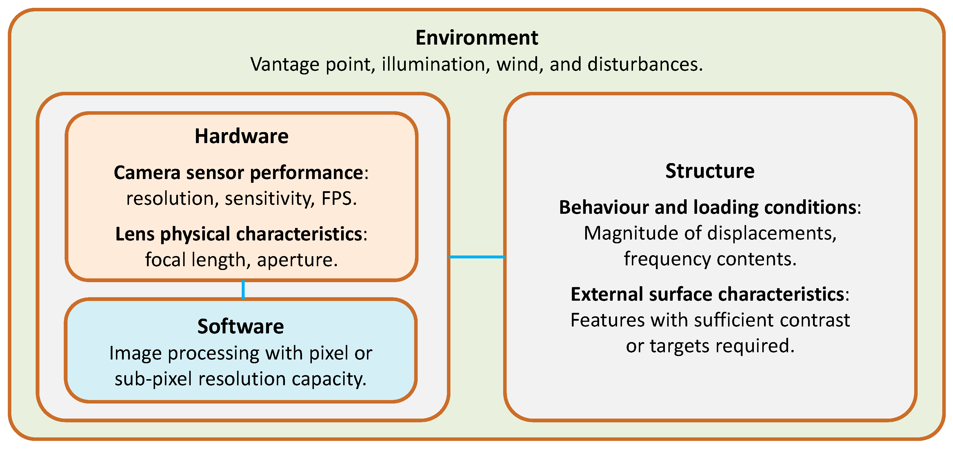
  • The absolute displacement (spatial) resolution depends on the environment (distance of the camera from the target) as well as on the hardware and software specifications/settings.
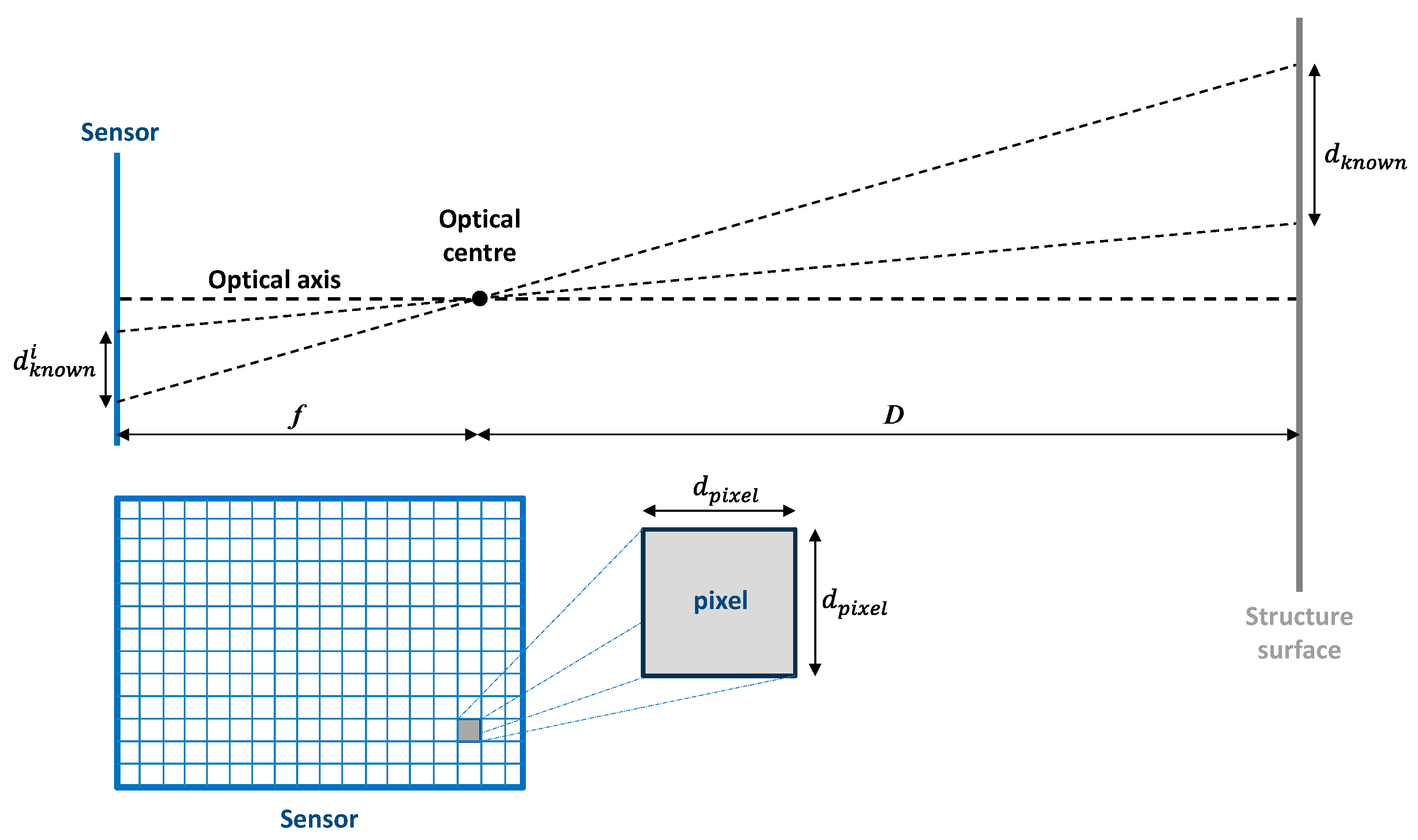
  • The scale factor (SF), defined as the ratio between the physical dimension and pixel number, is determined by the sensor pixel dimensions (hardware specifications/settings), the distance of the camera from the target (environment), and the focal length of the adopted lens (hardware specification) in the case of an optical axis perpendicular to the surface of the structure being monitored.
  • Although the condition of an optical axis perpendicular to the structural surface is very difficult to be satisfied in many real conditions, studies on the influence of the tilt angle [1] showed that errors in displacement estimation are not significant in practical applications, e.g., about 1% for a tilt angle of 30° when using a 50 mm focal length. In addition, it was found that errors are reduced when the focal length increases. Accordingly, inaccuracy from optical tilt angles can be generally neglected.
  • The SF alone provides partial indications on the absolute displacement resolution given that the adopted image processing algorithm has a key role, depending on its subpixel resolution identified through an upsampling factor, e.g., [35,36,37,38,39].
  • More important than the absolute displacement resolution is the resolution relative to the magnitude of the displacements being monitored in the structure, which depends on the structural stiffness properties and loading conditions.
  • The frequency of data acquisition is determined by the hardware (sensor sensitivity and lens light-gathering ability) and by the environment (illumination conditions). For example, for a given illumination intensity, a sensor with higher sensitivity allows a shorter exposition time and, hence, more frames per second (FPS) can be recorded; the same goes when using a lens with a smaller focal ratio, i.e., the ratio between the focal length and aperture diameter, gathering more light and, accordingly, permitting a shorter exposition time.
  • High values of FPS might be incompatible with real-time tracking elaboration of displacements, depending on the speed of the processing software and hardware being used. If this is the case, only structural monitoring based on the post-processing of video footages might be used.
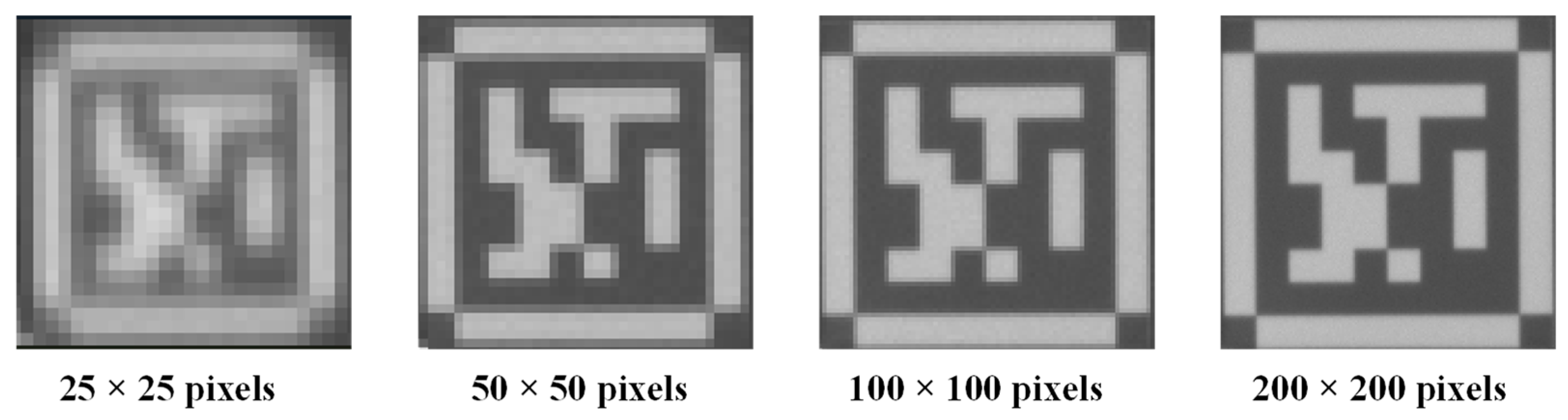
  • The type of targets, i.e., artificial (high-contrast markers) or natural (surface features), can have an influence on time resolution (a higher contrast permits a lower exposition time and hence a higher FPS) as well as on spatial resolution (properly dimensioned targets might maximise SF), with a non-negligible difference in terms of the final accuracy and repeatability of measures.
  • Image distortions could be induced by unfavourable environmental conditions such as heat haze; these distortions are inevitably amplified by the distance between the camera and the target (again an environmental factor). On the other hand, image distortions induced by the hardware have negligible influence, especially in the case of a high quality fixed-focal lens.
  • Other adverse environmental conditions might be vibrations transmitted to the camera, either by the ground through the tripod, by the connecting cables, or directly by the wind or other source of noise; the negative influence of vibrations induced in the video camera is amplified by the distance of the camera from the target and by longer focal lengths. Inevitably, the negative influence of noise induced by the surrounding environment are expected to affect more the measurements of small displacement magnitudes.
Some of the aspects listed above were investigated in previous studies using laboratory testing under controlled conditions as well as field testing, mostly involving steel bridges and footbridges [1,2,3,4]. While such studies constitute a very important background for vision-based monitoring systems, the analysis of their performance deserves further investigations, also considering the potentialities of future applications in continuous structural monitoring.
In this context, the attention here is focused on the application of a vision-based structural monitoring system to a medium-span, simply supported, post-tensioned concrete bridge. The reasons that motivated this experimental research activity are:
  • Few field studies using vision-based monitoring are available for concrete bridges which are the most widespread bridge solution in many road networks; for example, in Italy [40] and Europe [41].
  • In concrete bridges, the deflections expected are generally lower and their frequency contents generally higher as compared to those found in steel bridges investigated in previous studies; thus, concrete bridges are a more demanding testbed for vision-based monitoring.
  • The large number of concrete bridges built in the second half of the 20th century are approaching or are already at the end of their service life; thus, the demand for their monitoring is expected to rapidly rise in the near future [41]. Accordingly, a cost-effective monitoring solution providing comprehensive information has strategic importance for the security of our infrastructures [42,43,44,45,46,47,48,49,50].
The original contributions of this study aim at providing practical support to structural engineers interested in applying vision-based monitoring, and can be summarised as follows:
  • Analysis of the performance of a cost-effective vision-based monitoring system as compared to a system based on contact sensors, considering the influence of the operator and hardware settings.
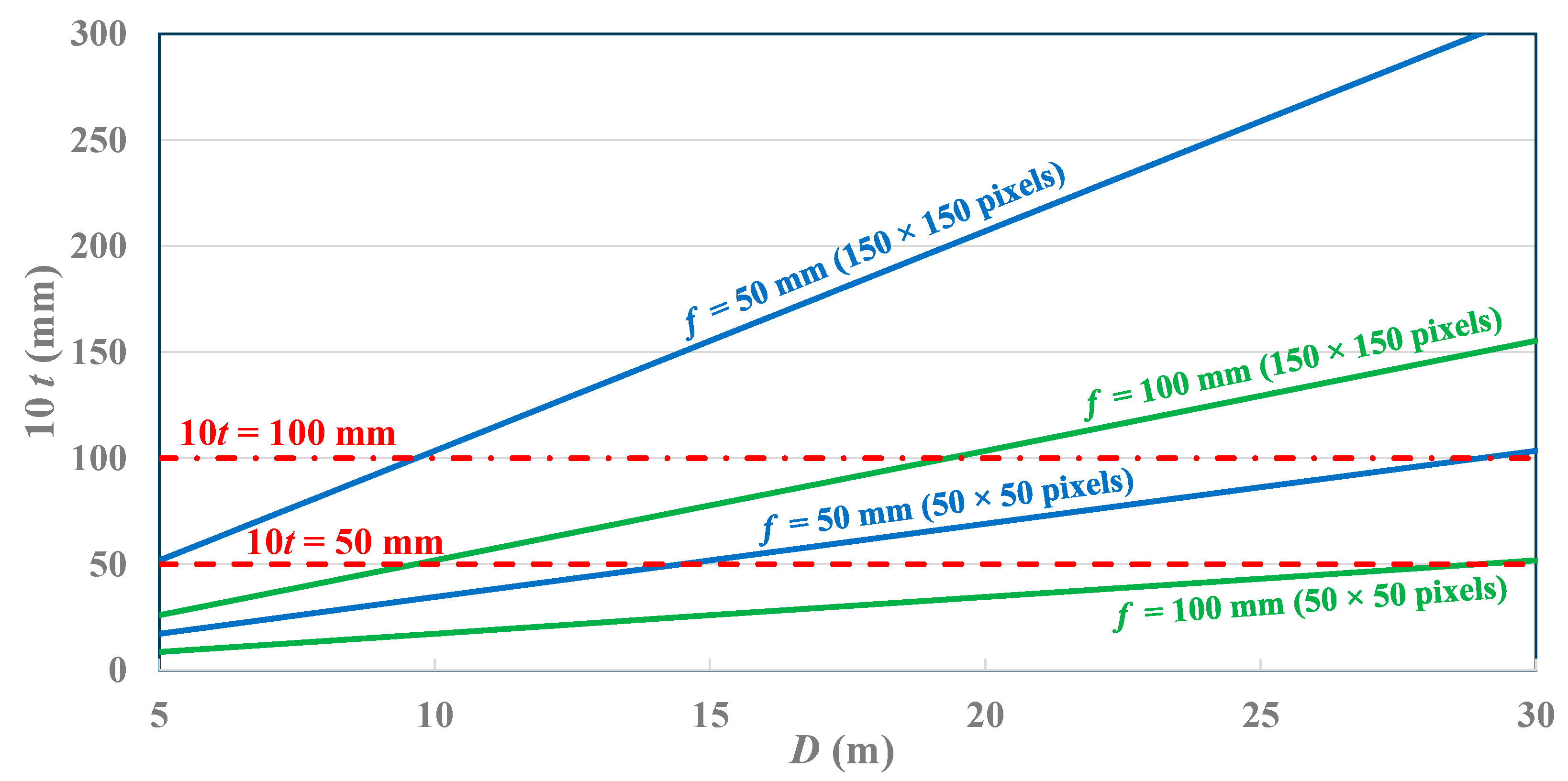
  • Indications for the optimal design of targets and the definition of the target area as a function of sensor resolution, distance of the camera from the target, and available focal lengths.
  • Identification of the physical and technological limits of a vision-based structural monitoring system in real-world field conditions.

2. Materials and Methods

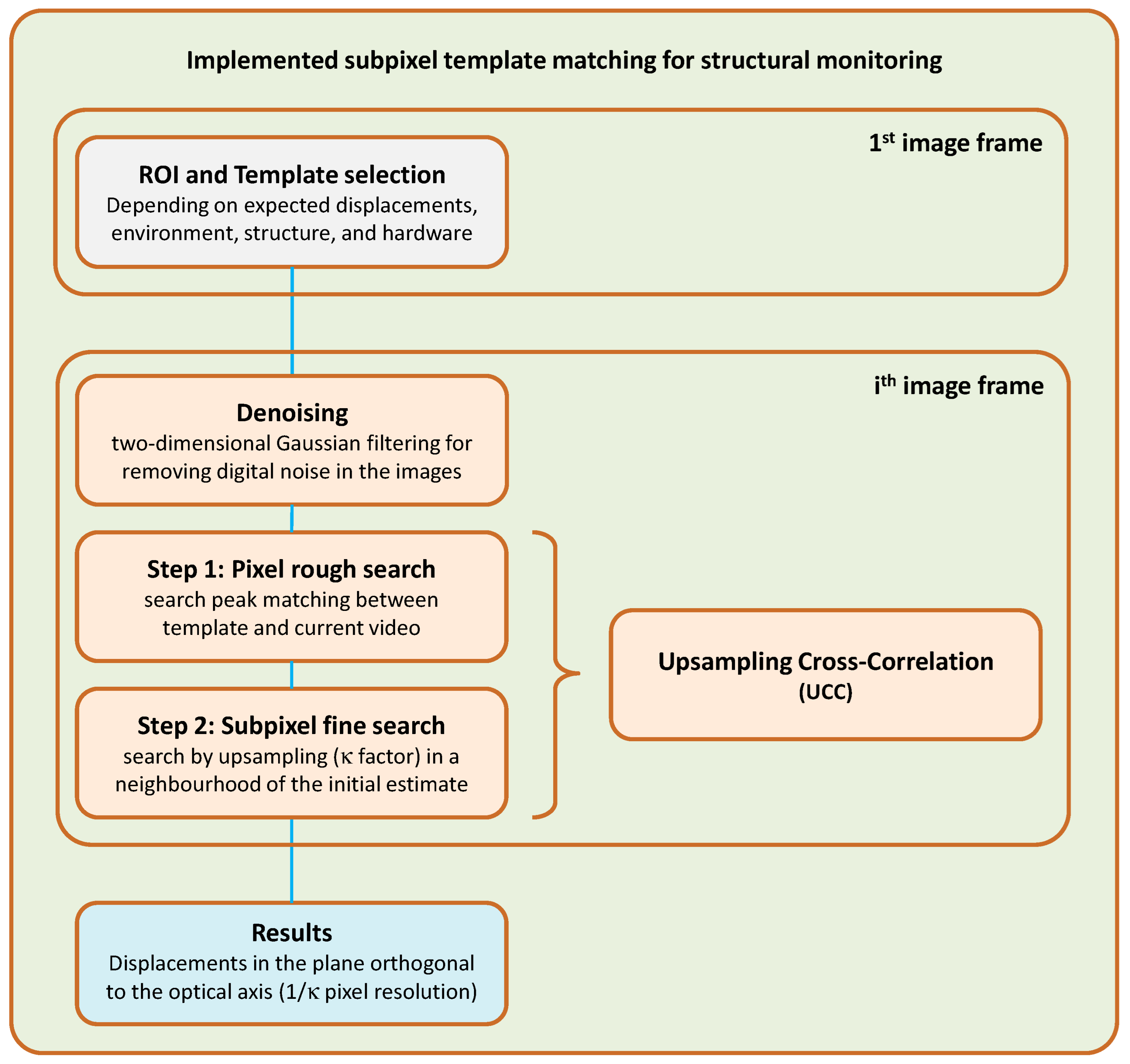
2.1. Image Acquisition and Processing Procedures

A real-time video processing software was implemented in MATLAB [51], taking advantage of its computer vision toolbox [52] as well as of the Generic Interface for Cameras (GenICam) protocol [53]. The extraction of displacement time histories exploits a template matching algorithm in the version originally proposed in [35] and available as a MATLAB code [54]. The algorithm is based on a cross-correlation peak matching, called upsampling cross-correlation (UCC), between a template selected by the user and each subsequent image of the video footage. The UCC template matching is intensity-based, i.e., the information of the image is mainly related to local intensity differences; hence, it is expected to better perform in case of high-contrast targets. The implemented procedure is exemplified in Figure 2 and can be subdivided in the following workflow:
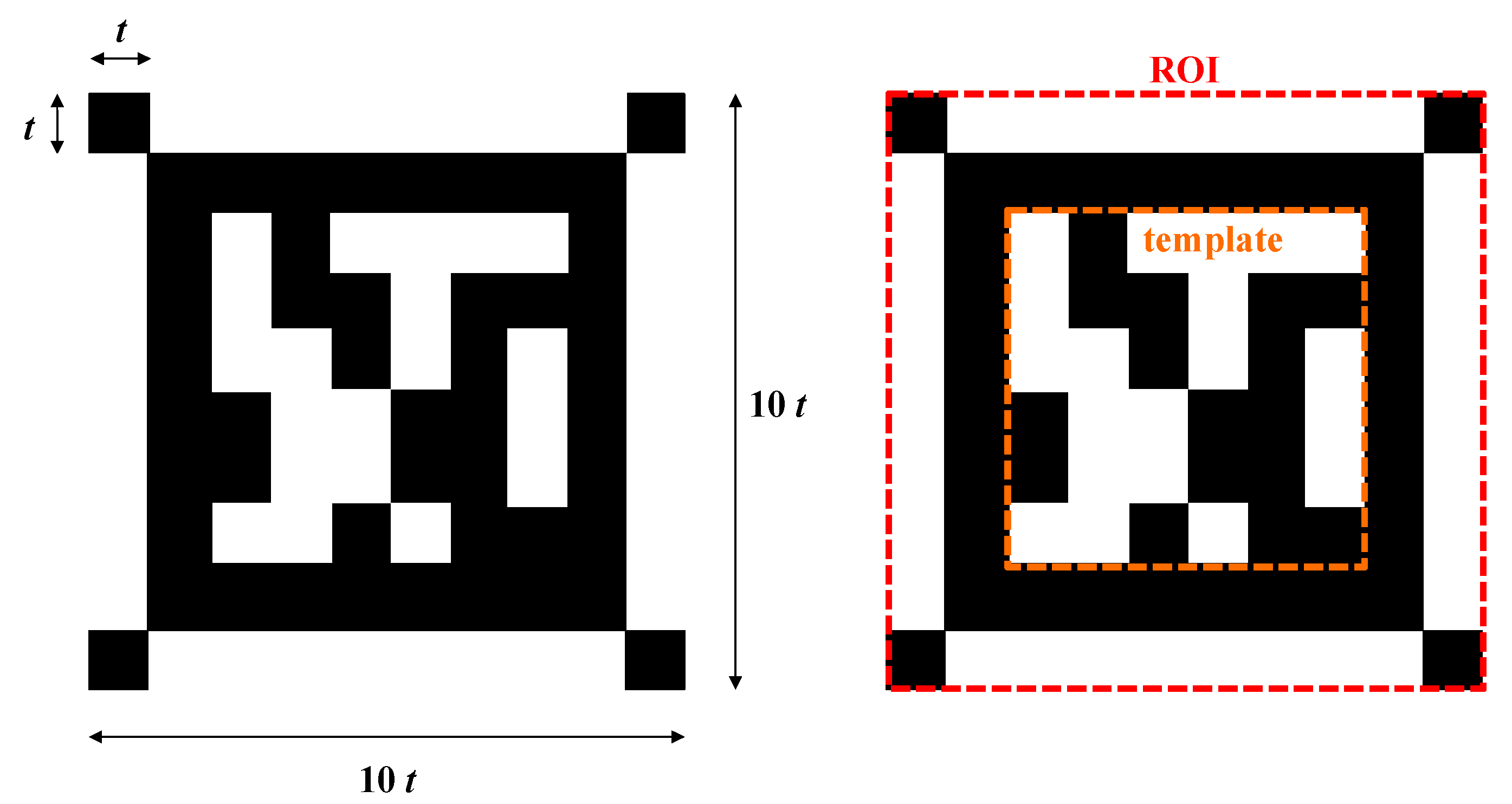
  • A portion of the image frame, called the Region of Interest (ROI), is selected by the user and within the ROI a template is chosen. The motion of the template will be tracked only in the ROI; hence, the margin between the template and ROI must contain the maximum displacement that will be experienced during monitoring.
  • Digital noise in each image frame is reduced prior to the application of the template matching algorithm through two-dimensional Gaussian filtering as implemented in MATLAB [51]. Such image denoising was found to be very beneficial in reducing the noise of the extracted displacement time histories.
  • Cross-correlation peak matching is performed to identify the displacement of the template within the ROI in two steps: (1) a pixel-level rough search providing a preliminary estimation of the displacements with pixel resolution; (2) a subpixel fine search within a neighbourhood of the initial estimation achieving 1/κ pixel resolution where κ is the assigned upsampling factor (integer value). Analytical details can be found in [1,35].
  • The extracted displacements in two orthogonal directions in the plane perpendicular to the optical axis are given as the final output.
The UCC algorithm is very efficient in terms of computation time and memory requirements, making its use potentially compatible with real-time processing, especially if small ROIs are selected. The continuous flow of frames is first hosted in a buffer and then directly elaborated and plotted during the video acquisition, allowing online visualisation of the measured displacements. The data saved are only the bidirectional displacement of each template while the single frames acquired are discarded, with significant savings in terms of data storage. A control procedure was implemented to check if the hardware can process the images hosted in the buffer with sufficient speed to avoid buffer memory overflow. If computer memory problems are detected by the implemented code, the user is requested to select a smaller ROI or a lower FPS to reduce the processing burden on the adopted hardware.

2.2. Vision-Based Hardware

The vision-based monitoring system used in this study consists of an industrial video camera for computer vision with an interchangeable C-mount lens (Table 1), installed on a tripod, and connected to a laptop through USB3.0. This system is basically a more recent version of the one adopted by Feng and Feng [3] in most of their applications in the United States. Complete technical specifications for the adopted camera can be found in [55].
The video camera sensor is monochrome, and this is a benefit over colour sensors. In fact, colour images are not required as they do not add information to the adopted algorithms for displacement tracking with respect to grayscale images. More importantly, a monochrome sensor has a higher quantum efficiency and a wider wavelength response curve that extends up to the near infrared region compared to its equivalent colour counterpart [56]. Thus, a better video sensor performance is expected and there is no need to use a conversion algorithm from colour to grayscale image frames prior to video processing.
Regarding the image acquisition, the adopted video camera uses the global shutter readout method, i.e., all sensor pixels are read out simultaneously; hence, images constituting the video footage are snapshots at the same time instant [57]. In this way, artifacts in moving objects (called motion blur) do not occur, as is instead the case in rolling shutter acquisition, i.e., sensor pixels are read row by row, as generally found in consumer video cameras.
The use of a fixed focal lens was preferred over a zoom lens for several reasons. While a zoom lens might appear more practical for the possibility of tailoring the field angle without moving the camera, a fixed focal lens generally has a much better optical performances for the same cost and is more widely available in C-mount catalogues. However, the main reason was relevant to the need of having a known value of the adopted focal length to be used for the calculations discussed in the following section.

2.3. Scale Factor and Resolution

SF (the ratio between the physical dimension and pixel number indicated as variable RSF in the following equations) can be obtained from the distance between the camera and the target (D), the focal length of the lens (f), and sensor pixel size (dpixel):
R S F = D f d p i x e l
as derived from the following geometric relations (Figure 3):
R S F = d k n o w n I k n o w n = d k n o w n d k n o w n i / d p i x e l
d k n o w n d k n o w n i = D f
where d k n o w n is the known physical length of an object in the image, d k n o w n i is the corresponding length of that object in the image plane, and I k n o w n = d k n o w n i / d p i x e l is the matching number of pixels.
In the case of pixel-level search (the first step of the cross-correlation peak matching previously described), RSF is the smallest displacement Rdisp (displacement resolution) that can be detected, i.e., one pixel represents a physical displacement equal to RSF. The addition of algorithms with subpixel accuracy, as is the case of this study, reduces Rdisp according to the following formula:
R d i s p = R S F κ = D κ   f d p i x e l
where κ is the upsampling factor. Hence, a lower value of Rdisp can be achieved reducing the distance D between the camera and the target, using a longer focal length f, adopting a higher upsampling factor κ, and using a video camera with a smaller pixel size dpixel. For example, in the case of the video camera adopted in this study (dpixel = 3.45 µm), setting D = 10 m and f = 100 mm gives RSF = 3.45 × 10−3 mm × 10,000 mm/100 mm = 0.345 mm, i.e., a single pixel in the acquired image represents a physical square of 0.345 mm side. If κ = 100 is assigned, then Rdisp = 0.00345 mm.

2.4. Target Design

The choice of a proper target is an important aspect for three reasons: (1) its major influence on the efficiency and accuracy of the template matching algorithm; (2) its significant facilitation of the camera calibration procedures for determining SF; (3) its function as a guide for the optimal selection of the ROI and template. This is especially true in the case of concrete bridges where it is generally very difficult to extract portions of the visible surface that have known dimensions and that could be clearly recognized (in steel bridges, the presence of stiffening plates, bolts, and nuts could be useful in that sense). Accordingly, in this study only template matching using artificial targets is considered.
Various targets were utilised in previous applications [1,2,3,4,5,6,7,8,9,10,11,12,13,14,15,16,17,18,19,20,21,22,23]; however, no recommendations or proposed target design rules can be found for structural monitoring applications. Therefore, a practical target design is proposed here having as objectives the efficiency and accuracy of the template matching algorithm, the support in camera calibration, and the optimal selection of the ROI and template.
The proposed target has a square shape subdivided in a 10 × 10 chessboard, for a total of 100 squares with local dimension t. Hence, the target has an overall dimension 10t. The 36 edge squares are white except for the four squares in the corners that are black. The internal portion is made by 8 × 8 = 64 squares that are black except for a portion of the 6 × 6 = 36 internal squares that are white and define a pattern. Different internal patterns can be used to identify the monitored points if multi-target monitoring is carried out. An example of the proposed target is shown in Figure 4.
The outer part is intended to guide the definition of the ROI while the internal portion can be entirely or partially selected as a template, as illustrated in Figure 4, depending on the expected displacements. In fact, the space between the edge selected as the ROI and internal portions selected as the template must be compatible with the magnitude of displacements, as previously explained, given that the template matching algorithm searches the template position within the ROI.
The design of the proposed target requires the definition of its global dimension (overall size) and local dimension (chessboard size). These geometric design parameters are influenced by the environment (distance D between camera and target) and the hardware (lens and video camera specifications). The global dimension of the target can be defined based on a requirement of compatibility with the field of view (FOV) of the adopted combination of camera and lens. This simply means that the target must be small enough to be entirely visible and large enough to be clearly visible. However, an appropriate design of the global dimensions is a necessary but not sufficient condition. In fact, the local dimensions must be selected so that the chessboard is visible with sufficient resolution for the proper identification of the target during setup and camera calibration as well as for allowing the correct operation of the UCC template matching.
In the proposed target, the local dimension t is the only design variable. Such a dimension can be obtained for the assigned values of D, f, dpixel, and the number of pixels required for the target to be clearly visible. Based on experimental evidence using the adopted vision-based hardware, the optimal discretisation for the ROI was identified as 100 × 100 pixels, balancing the clarity of the target chessboard and the computational effort. While increasing the pixel discretisation is a matter of higher processing and memory use (with a negative impact on the possibility of real-time monitoring for high FPSs and/or multiple points), the lowest pixel resolution identified to allow reasonable camera calibration with the adopted hardware is 50 × 50 pixels. See for example the results in Figure 5 obtained pointing at the target of Figure 4.
Allowing a ±50-pixel variation with respect to the optimal solution with 100 × 100 pixels, the suggested discretisation for the ROI is in the range 50 × 50 to 150 × 150 pixels. Accordingly, using Equations (1)–(3), setting Iknown = 50 pixels (lower bound) and 150 pixels (upper bound), f = 50 mm and 100 mm, D in the range 5 to 30 m, and dpixel = 3.45 µm, the graphs in Figure 6 are obtained. Figure 6 can be used to choose the dimension of the proposed target for a given distance D in relation to the available focal lengths or evaluate the range of applicability of a given target. For example, the proposed target with 10t = 50 mm has a wide range of applicability spanning about 5 to 14.5 m if f = 50 mm is used and about 9.5 m to 29.5 m if f = 100 mm is used; a target with 10t = 100 mm spans about 9 m to 29 m if f = 50 mm, as exemplified by the red lines in Figure 6. Similar graphs for different distances and focal lengths, not reported here, can be easily obtained to cover different situations and hardware specifications.

3. Experimental Campaign

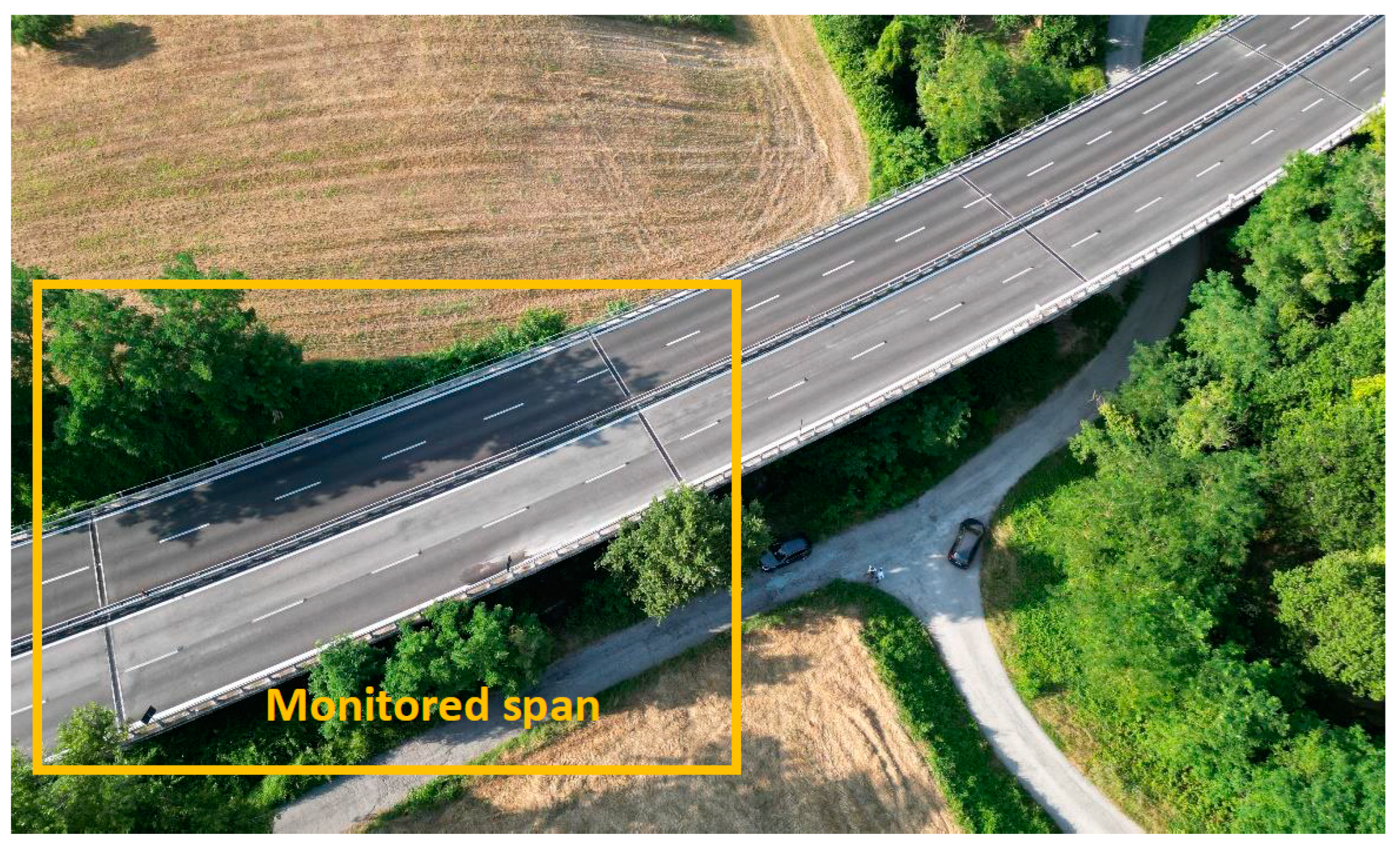
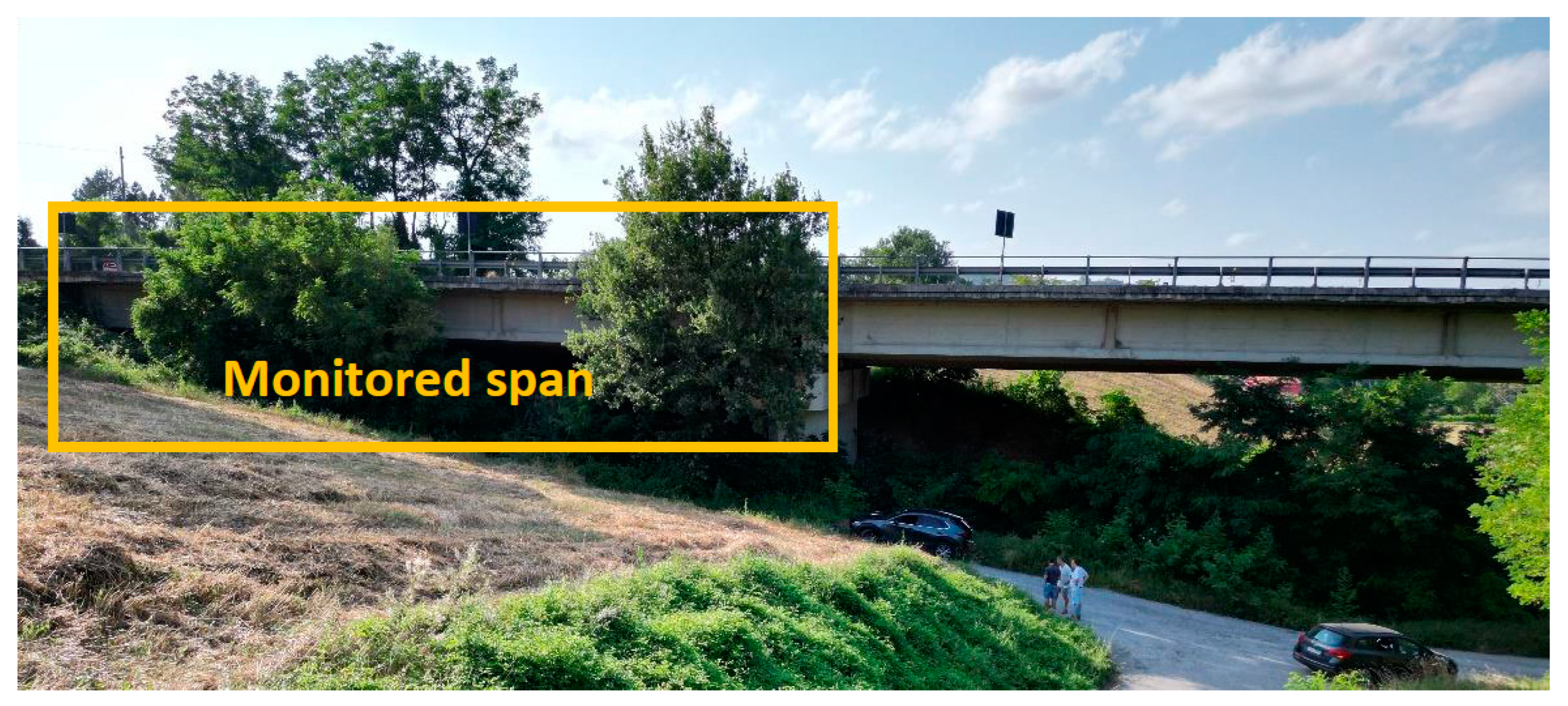
3.1. Case Study Bridge

The considered case study is a three-span concrete bridge located in central Italy, part of the national highway road network. Each span has a single deck made by a concrete slab on six simply supported post-tensioned concrete beams (span length 32 m) connected by end and intermediate transverse beams located at about 1/3 and 2/3 of the span. An aerial view of the bridge is reported in Figure 7 while a lateral view is given in Figure 8 (west on the left and east on the right). The west first span of this bridge was selected as a benchmark test of this study given its reduced distance from the ground at midspan, making possible a simple installation of displacement transducers for comparative purposes. The measurements of the bridge structural response illustrated in this study were conducted on July 20th, 2023, while the bridge was normally operational with regular vehicular weekday traffic, mostly cars and a limited number of heavier tracks.

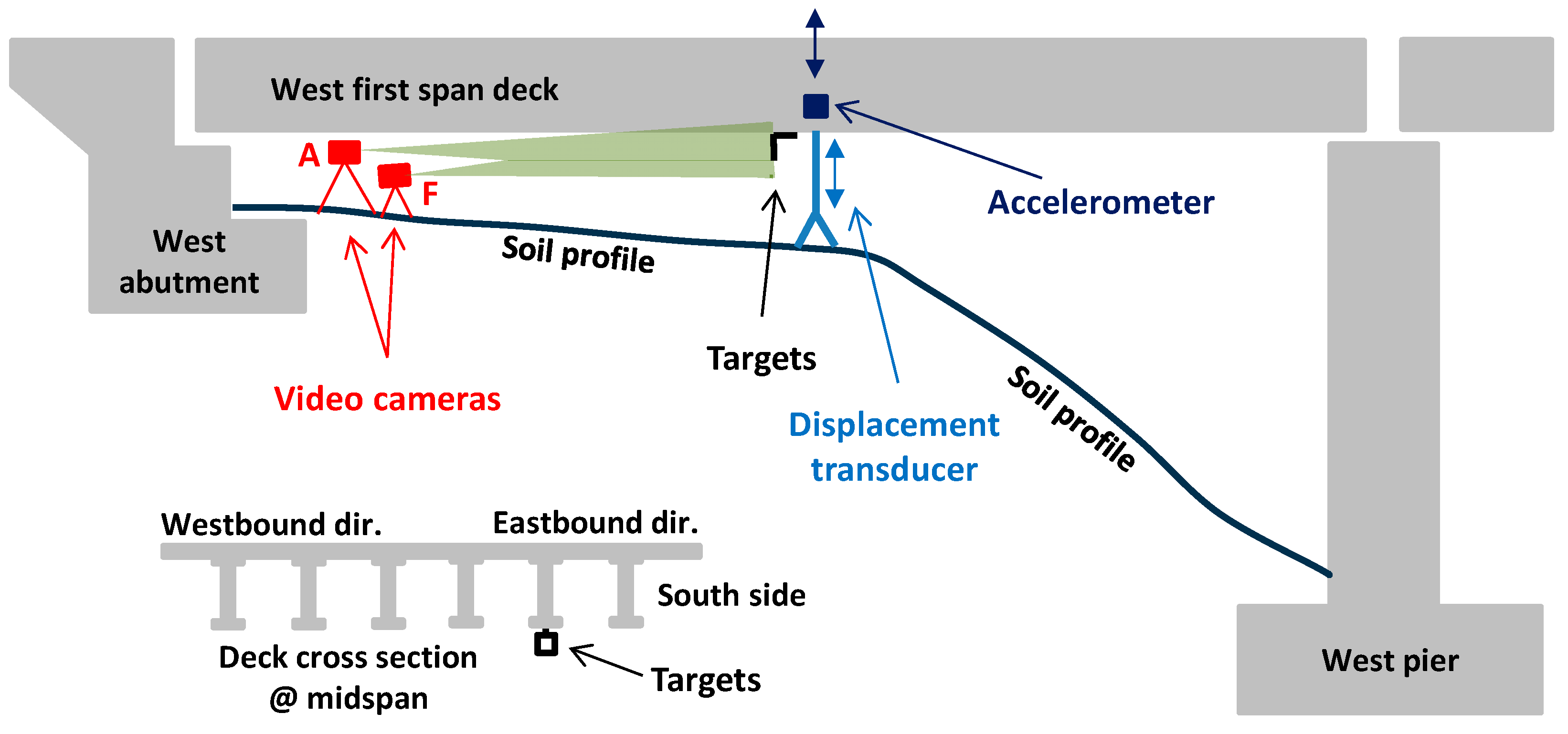
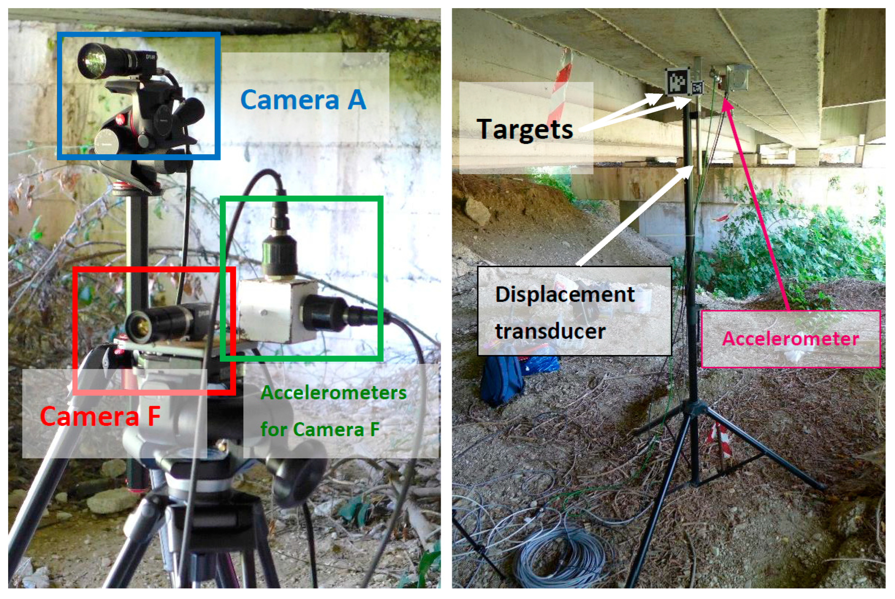
3.2. Vision-Based Hardware Installation

Two identical video cameras were placed under the bridge deck, near the west abutment, as depicted in Figure 9. Such a vantage point was selected as it is protected from rain and direct sunlight, potentially functional in future permanent monitoring applications. Specifically, the two cameras were positioned under the second beam in the south side of the deck (Figure 9); camera A at 12.40 m from the target and 20 cm below the deck on a high-quality aluminium photo tripod (mass 3.25 kg), camera F at 12.10 m from the target and 60 cm below the deck on a high-quality aluminium video tripod (mass 5.50 kg). Two targets (10t = 50 mm and 10t = 100 m) were attached at the midspan of this same second beam using an L-shaped metallic support fastened to the post-tensioned concrete beam. The optical axis is nearly parallel to the bridge axis; accordingly, both the vertical and transverse displacements of the intrados of the beam can be traced (nonetheless, attention in this study is on the vertical deflection only). Figure 10 shows the two video cameras during acquisitions (left-hand side picture) and the targets at midspan (right-hand side picture).

3.3. Contact-Based Hardware Installation

A high-precision linear variable displacement transducer (Gestecno TSL-160, Gestecno, Castelraimondo, Italy) was installed at the midspan using a stiff tripod anchored to the ground through steel bars inserted into the soil for about 1 m (Figure 10). The transducer has a 100 mm displacement range, 0.20% accuracy, 0.01 mm repeatability, and was calibrated before this experimental campaign. As previously mentioned, this installation was made possible thanks to the limited distance (about 1.8 m) between the beam and the ground. A high-sensitivity piezoelectric accelerometer (PCB 393B31, PCB Piezotronics, Depew, NY, USA) measuring vertical accelerations was fastened at the midspan, very close to the displacement transducer (Figure 10). In addition, a sensor for air temperature and relative humidity (RH) with integrated data logger (Elitech RC-51H, Elitech, London, UK) was placed at the midspan, on the flange of the beam, near the displacement transducer and accelerometer, and programmed to record its readings at 15 min intervals.
Two piezoelectric accelerometers (PCB 393A03) were connected to the top of the tripod of video camera F (Figure 10) to measure accelerations in the plane perpendicular to the optical axis, with the goal of quantifying possible undesired vibrations next to the video camera that could have negative effects on the accuracy of the extracted displacement measurements. It is noted that with this installation, a 2.90 kg mass due to the two accelerometers and the adopted metallic cube (Figure 10) was added to the top of the tripod of camera F.
The signals of the displacement transducer and accelerometers were acquired using a high-performance data logging system (Dewesoft Krypton) and its controlling software (Dewsoft X 2023). Their acquisition sampling frequency was set to 1200 samples/s.

3.4. Camera Calibration and Settings

Once the video cameras and the targets were installed, an operator oversaw the selection of the ROI and template as well as the camera calibration, i.e., the determination of SF. The preliminary step to this procedure was the selection of the lens focal length and target size. Preference was given in this experimental campaign to f = 100 mm, the longest focal length available at accessible costs for C-mouth video cameras, to achieve the most favourable SF. Such a focal length was combined with a target having 10t = 50 mm according to Figure 6 (D is about 12 m). Two other combinations were tested, i.e., f = 50 mm with 10t = 50 mm and 100 mm. Lenses were used at the maximum aperture (F2.8).
The determination of Iknown in Equation (2), required to calculate SF, was made measuring in the image the number of pixels for a given side of the target. In camera F, only one measure was used to count the pixels corresponding to the known length. In camera A, four measures for counting the pixels were taken, one for each side of the square target, and then Iknown computed as the average of the four measurements, compensating for possible differences determined by the vertical and horizontal tilt angles of the optical axis with respect to the direction perpendicular to the target. The objective of using two somewhat different procedures for calculating SF was the evaluation of such operational parameters, providing important indications on the repeatability of the vision-based measures.
During the preliminary operations, it was realised that, despite the sunny summer day, the targets had insufficient luminosity, mostly due to the dense vegetation and reduced space in the first half of the span (Figure 7 and Figure 8). This is a recurrent environmental condition under bridge decks and the use of targets printed on nonreflective material (regular white cardboard) did not help at this regard. Accordingly, a lamp was required to increase the illuminance of the targets from 150 lux under natural light (insufficient for having a clear view of the target during camera calibration and not providing enough contrast to allow the UCC template matching to work properly) to 2000 lux which allowed easy camera calibration procedures and the UCC algorithm to work without problems even for FPS above 120. Target illuminance was measured using a digital lux meter (TES 1330A).
Regarding the FPS settings, it must be remarked that the maximum frame rate of most consumer video cameras is in the range from 30 to 60 FPS; such speeds are indicated in the literature [1,2,3,4] to be sufficient for displacement monitoring, given that the midspan deflection is dominated by the first vibration mode [58,59]. Global shutter industrial video cameras such as the one adopted in this study allows for much higher speeds than consumer cameras, provided that the illumination conditions make it possible to use an exposure time that is compatible with the adopted FPS, e.g., a 500 FPS requires that the exposure of a single frame is equal to or less than 1/500 s = 0.002 s. Given this technical possibility, in this study the sensitivity of the experimental results to FPS from 30 to 240 were explored. The adopted case study appears an interesting testbed for the field evaluation of this aspect, given the expected higher frequency of the first vertical mode as compared to steel bridges and footbridges tested in other studies.

3.5. Field Measurements

The experimental measurements consisted of 10 min acquisitions simultaneously performed using the two video cameras and the contact sensors. The monitoring system based on contact sensors was assumed as the reference system and recorded the displacement transducer (DT), the accelerometer at midspan (AC), and the vertical and horizontal accelerometers on the tripod of camera F (ACTV and ACTH respectively). The two video cameras were used exclusively in real-time video processing for displacement extraction; thus, no memory-consuming video footages were recorded or stored.
The settings in the two video cameras are listed in Table 2. The labels AVB and FVB are used for the measurements derived from camera A and F, respectively. In camera A, the parameters were kept constant except for the fifth acquisition (AVB5) where FPS = 240 was used instead of 120. A new ROI and template selection was made at the beginning of each acquisition, thus resetting the previous choice. In camera A, effort was made to select the ROI and template as close as possible to the selection proposed in Figure 4 while in camera F slightly larger areas were adopted. The upsampling factor in the UCC template matching algorithm was set to κ = 100 for all acquisitions except for FVB1 where κ = 50 was used. The column “pixel search” reports the margin in the pixels between the template and the ROI and, hence, indicates in pixels the maximum displacement that can be measured. This number can be converted to a physical length by multiplying the “pixel search” by SF, a value always larger than the maximum displacements recorded by the reference contact-based monitoring system (later reported). Video camera A was not used in the seventh acquisition window due to accidental shortcomings in its controlling computer.

3.6. Signal Alignment

The measurements DT, AVB, and FVB were recorded using three different computers (one laptop for the contact sensors, two laptops each controlling one camera); hence, an alignment of the measures was necessary. The ordinates were aligned minimising the differences of the moving means of AVB and FVB with respect to the moving mean of DT taken as reference zero displacement. The moving means were evaluated on a 60 s mobile window using the MATLAB command “movmean”. Subsequently, the abscissas were synchronized adopting the MATLAB command “alignsignals” which estimates the delay between signals using cross-correlation [60]. Solely for this operation, the AVB and FVB signals were resampled at 1200 samples/s while the subsequent analyses were based on the non-resampled aligned signals. Following the displacement synchronisation procedure, the accelerometers synchronised to the two video cameras, being DT, AC, ACTV, and ACTH acquired by the same data logger.

4. Results

4.1. Environmental Conditions

The environmental conditions were basically constant in terms of recorded air temperature below the bridge deck while RH was initially decreasing and later increasing during the measurement campaign (Table 3). The solar radiation, mainly in absence of clouds, constantly acted on the extrados of the bridge, while all sensors and instruments were in the shade below the girder.

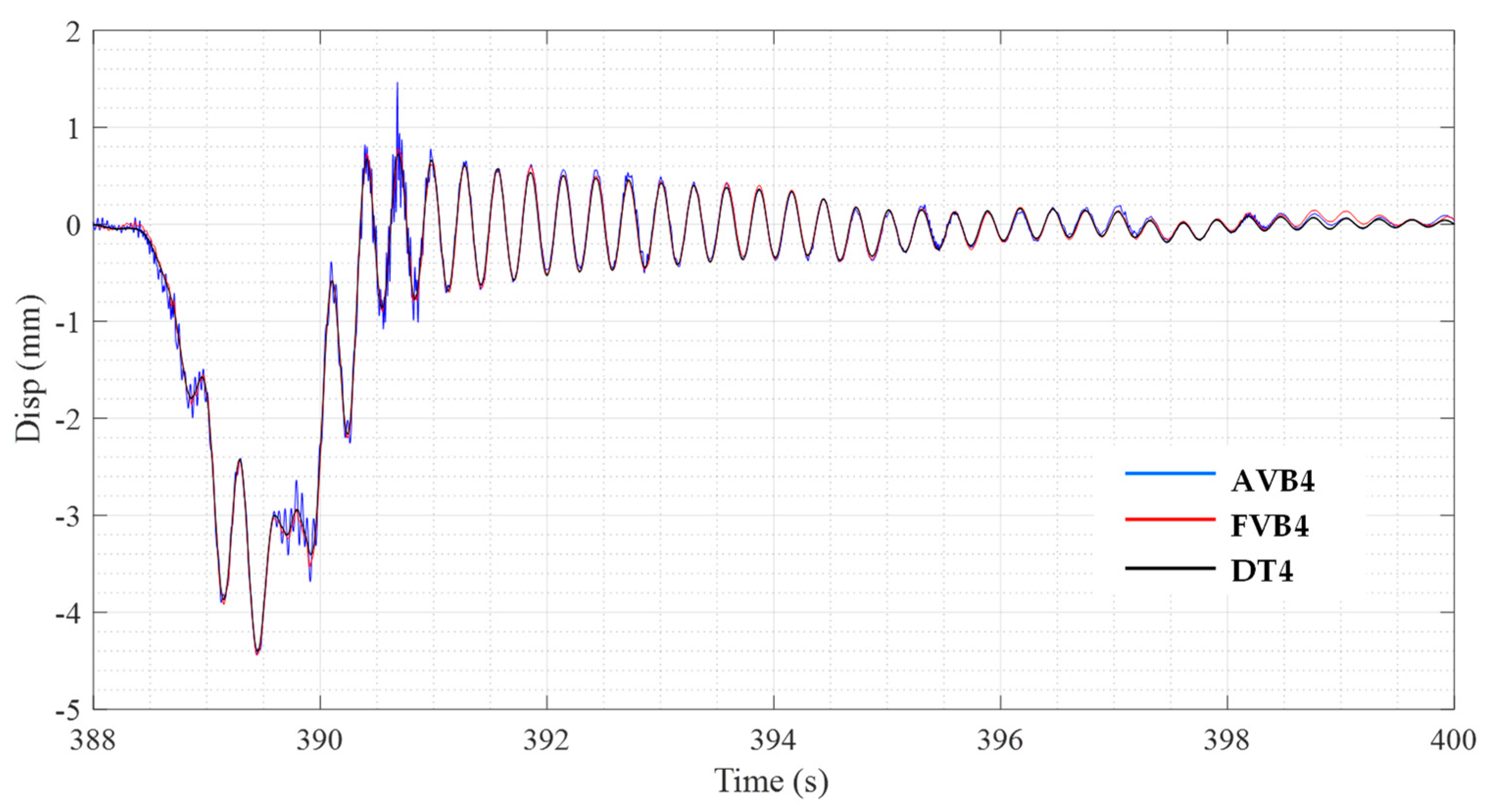
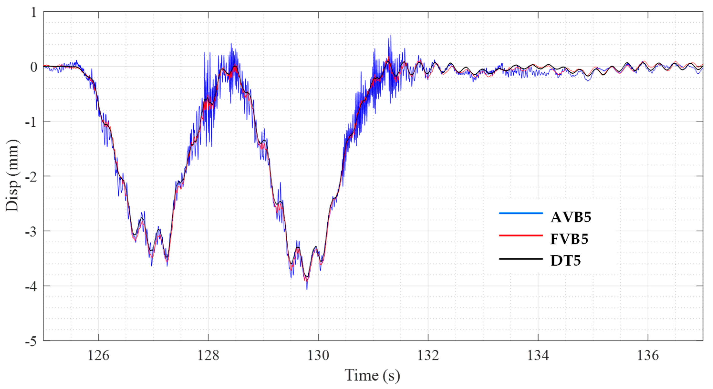
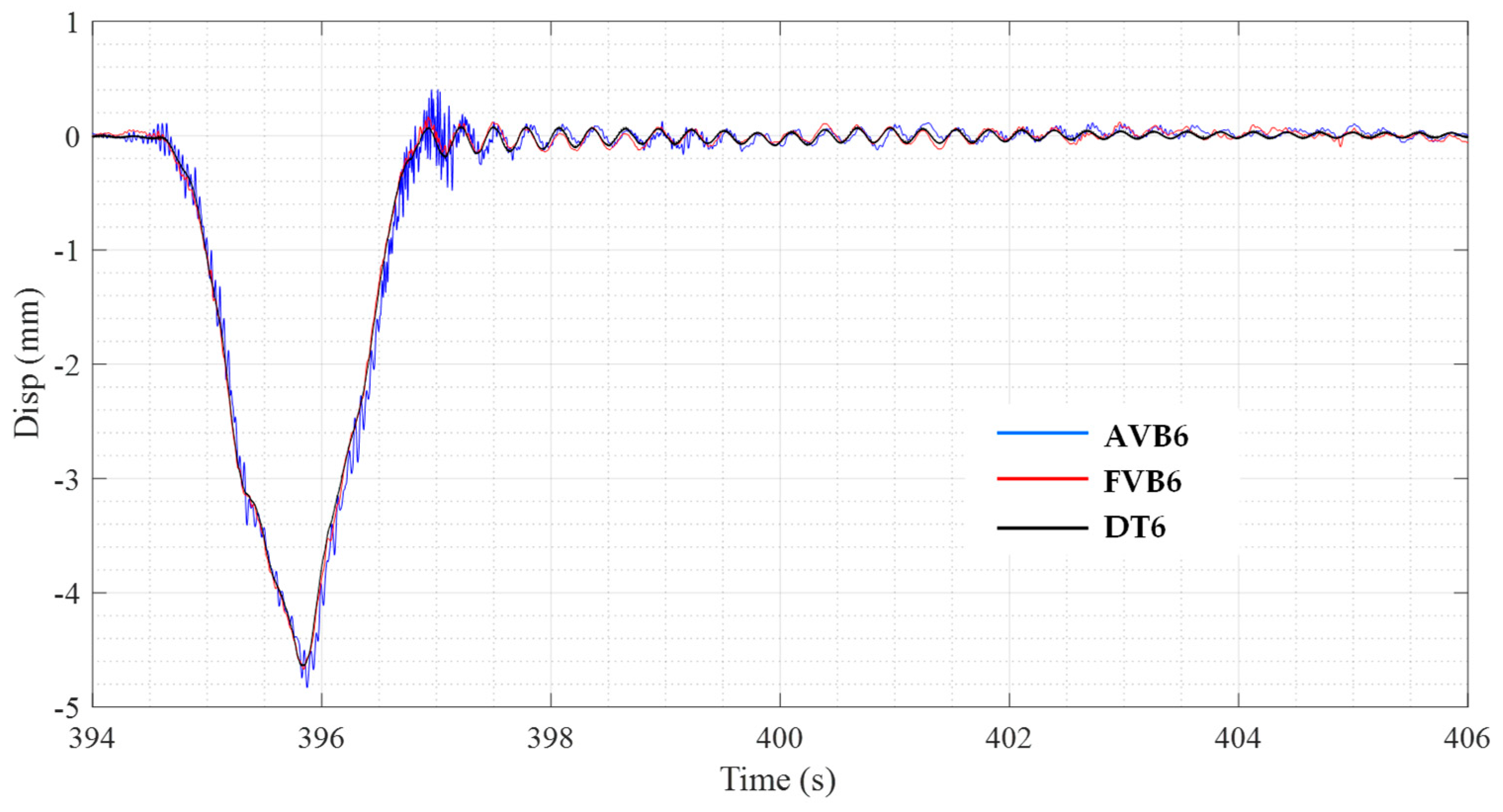
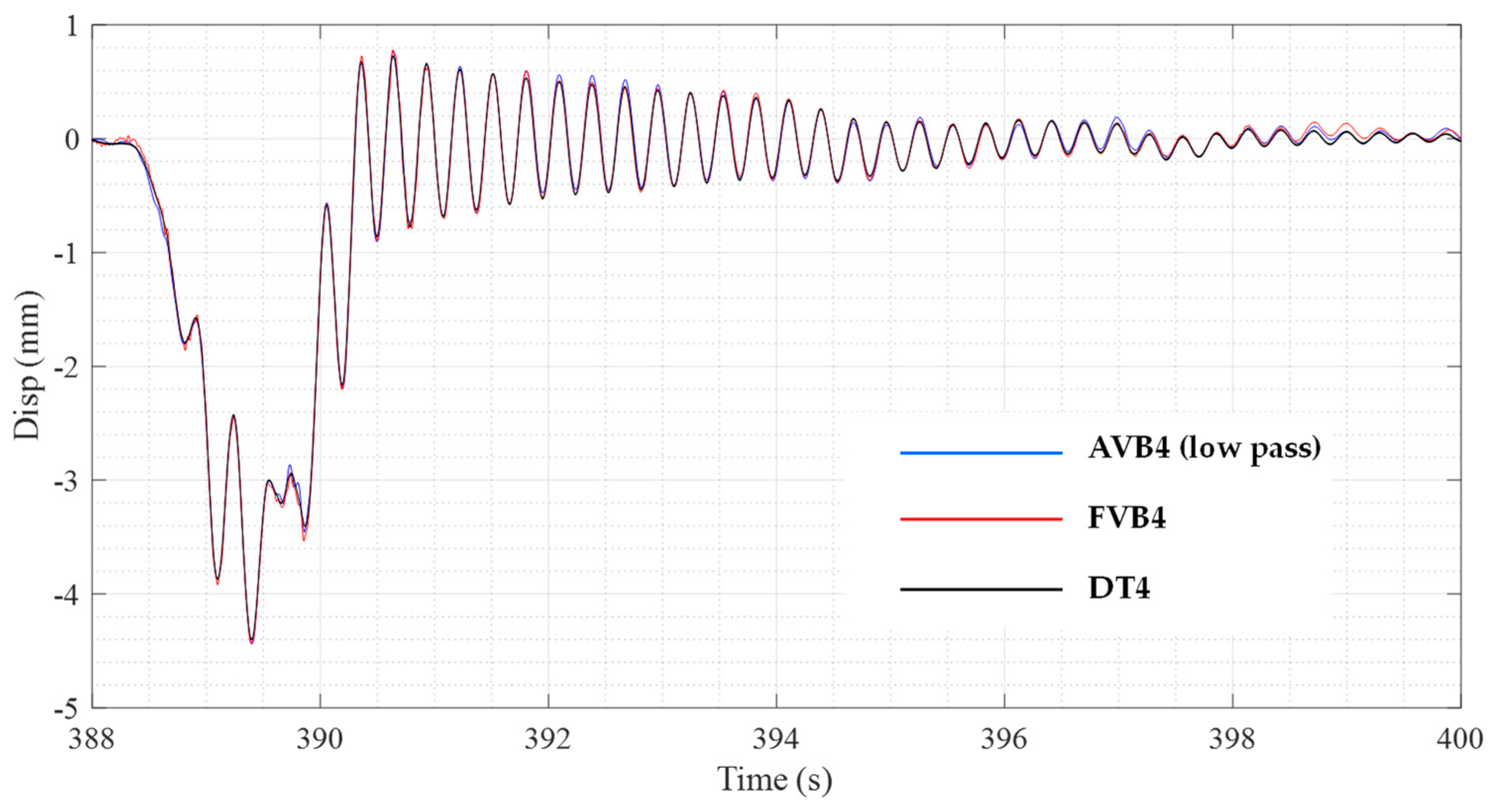
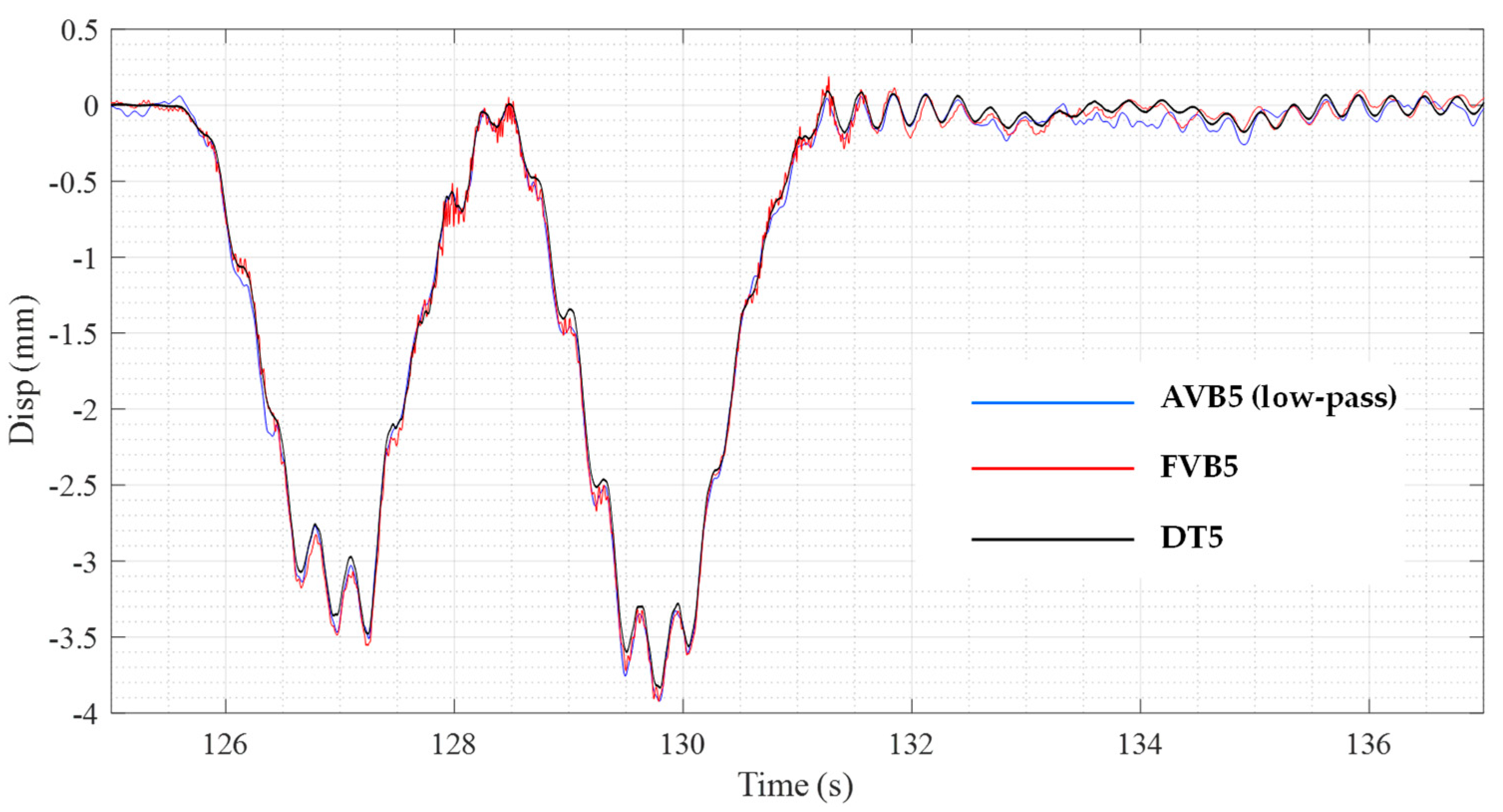
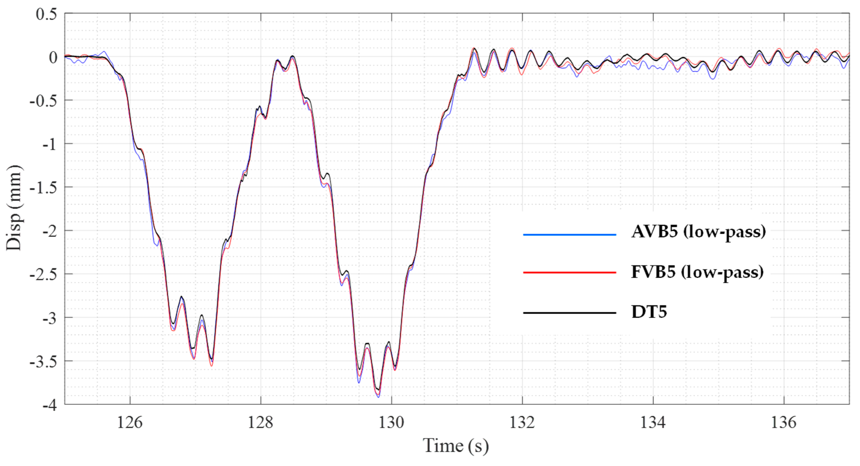
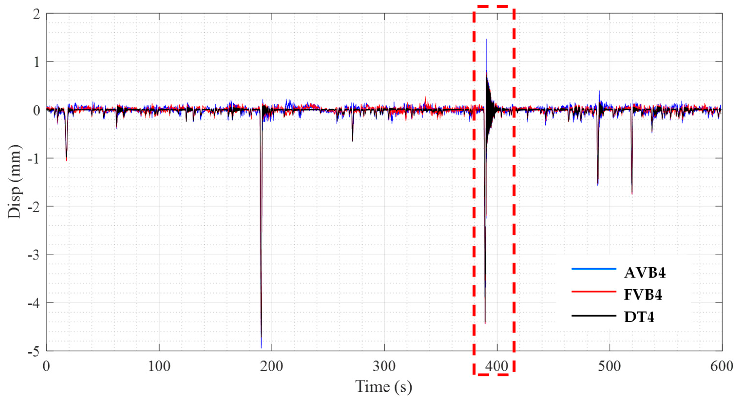
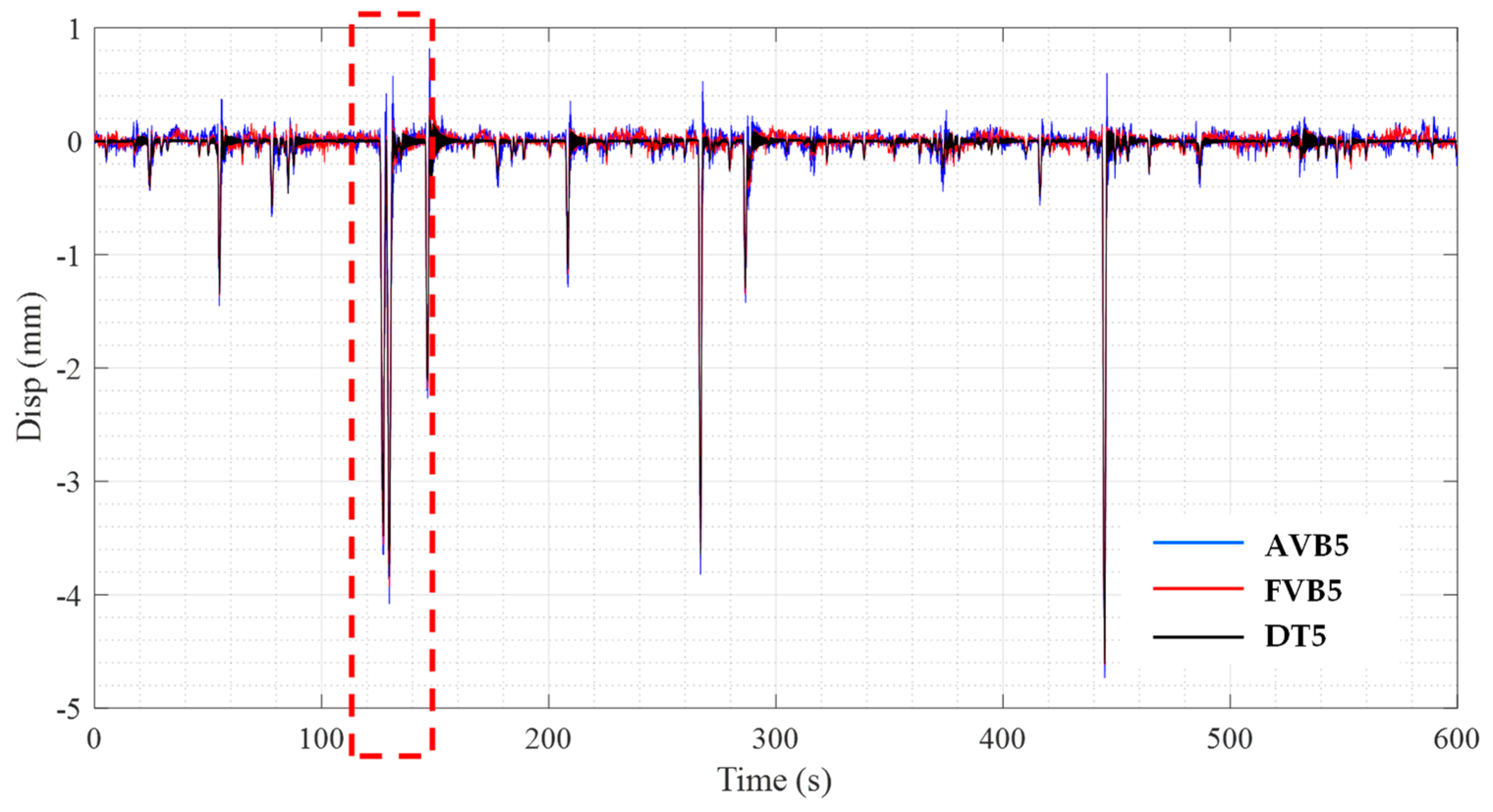
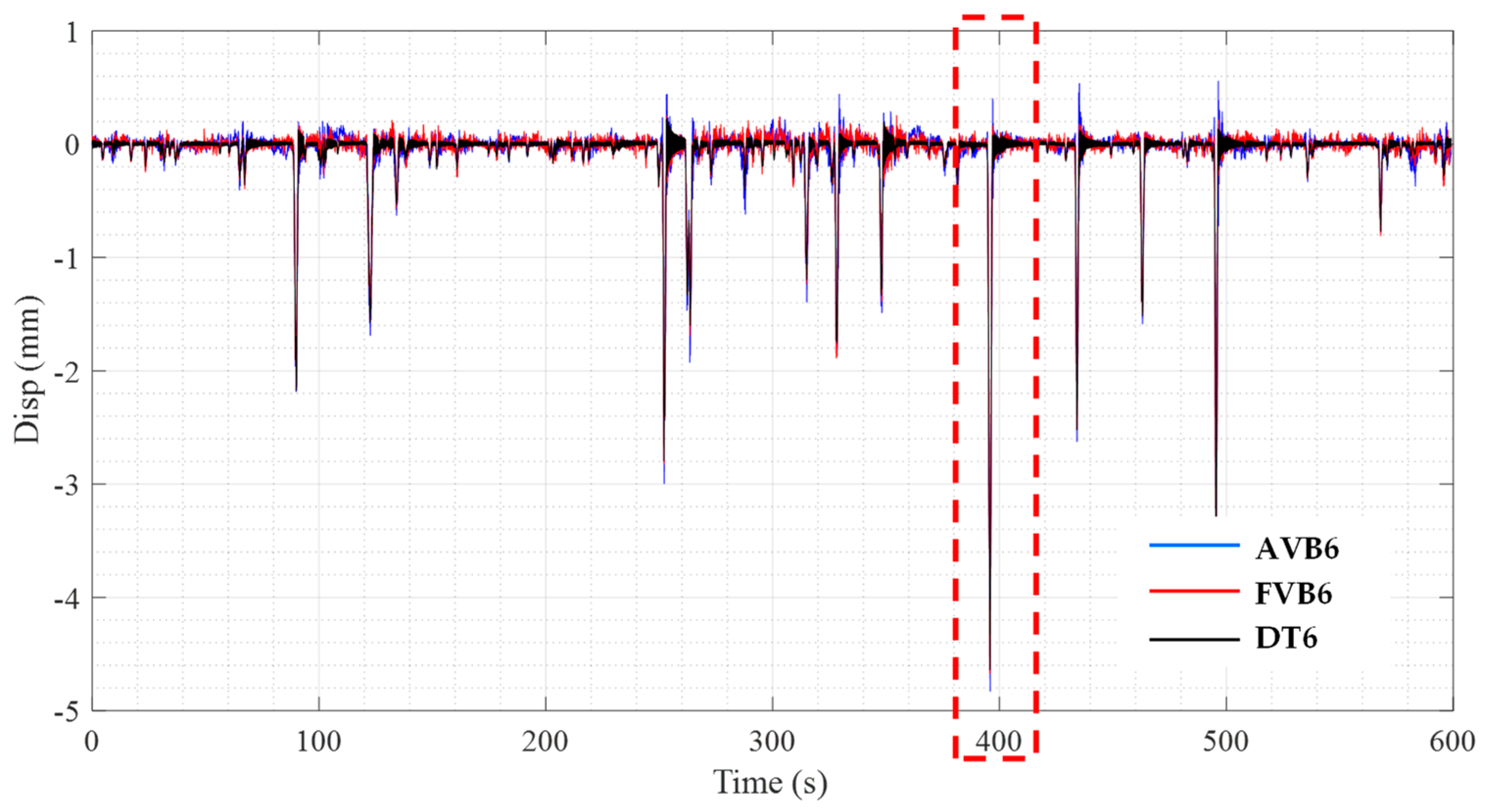
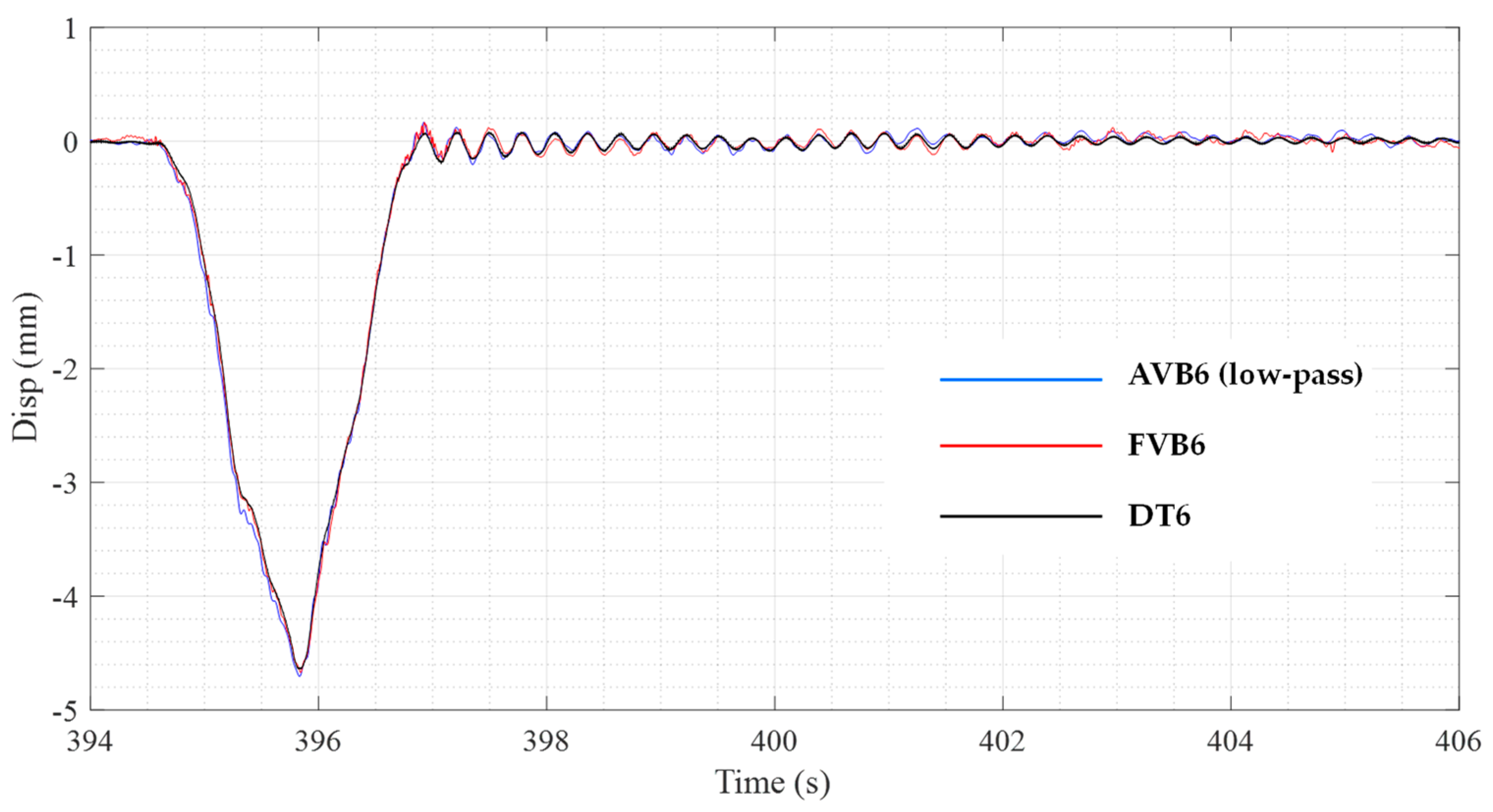
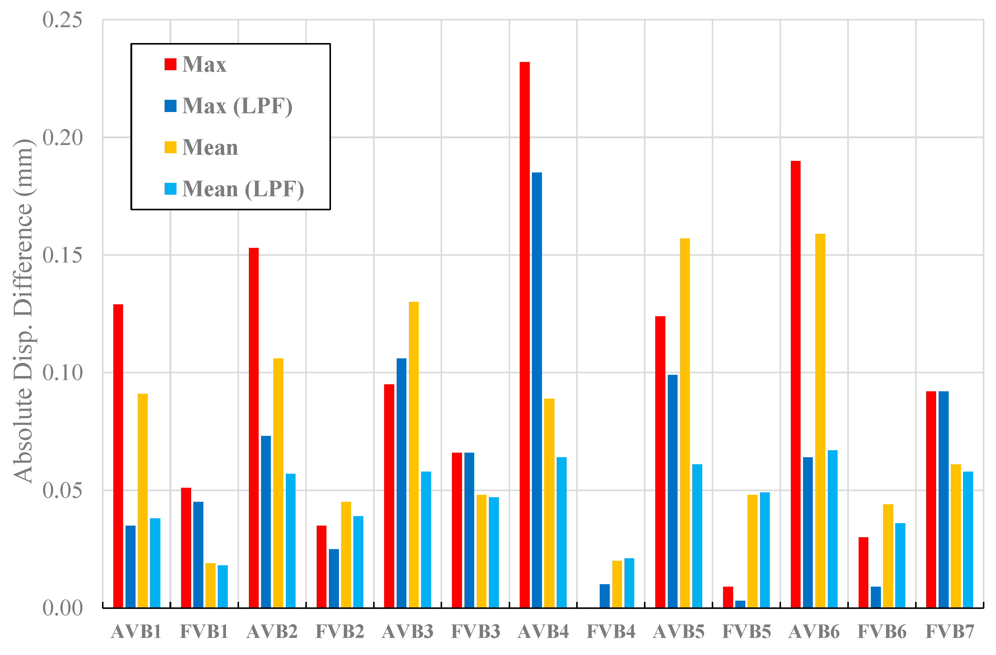
4.2. Analysis of Measured Displacements

Comparisons were made in terms of the displacements measured by the three systems within each of the 10 min acquisition windows. The results are summarised in Table 4 where the columns report from left to right the considered measure windows, the minimum displacement Rdisp that can be theoretically measured, the maximum displacement dmax that can be measured, the number of heavy vehicles defined as those inducing displacements larger than 1 mm, the maximum downward displacement at the midspan, the differences between vision-based and contact measurements of the maximum displacement (value and relative percentage), the mean and standard deviation of the absolute values of the differences between vision-based and contact-based measurements computed considering the maximum deflections determined by each heavy vehicle (for example, in the first acquisition window the mean and standard deviations are computed on four measures while the third window is on 24 measures).
The obtained results indicate that differences in terms of the maximum vertical displacements between contact-based and vision-based systems are small: the largest discrepancy is 0.232 mm in the case of AVB4 compared to DT4 (relative difference 4.92%) and the largest relative difference is 5.06% in the case of AVB1 compared to DT1 (discrepancy 0.129 mm). Systematic differences can be observed between the two cameras, even when the same parameters were adopted (AVB2 and FVB2), with camera F performing better than camera A if unfiltered raw signals are considered. Extensive analysis and discussion on these differences are hereafter presented, based on the direct comparisons of the extracted displacement recordings and analysis of the measured accelerations.
To gain more insight into the differences in the deflection measurements, some displacement time histories are shown in Figure 11, Figure 12, Figure 13, Figure 14, Figure 15 and Figure 16 (downward displacements have negative values in the graphs). The entire 10 min time range is given (Figure 11, Figure 13, and Figure 15) as well as abscissa close-ups in selected regions where heavy vehicles were driving (Figure 12, Figure 14, and Figure 16).
The displacement time histories show very small differences between DT and FVB along the entire dynamic response. On the other hand, the time histories AVB show that camera A is affected by high-frequency noise, more evident following displacement peaks. This disturbance is imputable to the vibrations induced by the vehicles and transmitted through the abutments and piers to the ground and hence to the camera tripod. While both video cameras were equally close to the west abutment (being the offsets between the two cameras 30 cm in the horizontal direction and 40 cm in the vertical direction, as already mentioned in the illustration of their installation), camera F was installed on a stiffer and heavier tripod that eventually filtered more effectively the external vibrations. More details on this issue are discussed in the following paragraph dedicated to the analysis of the measured accelerations. It is shown here the effect of the application of a low-pass filter (LPF) with cutoff frequency 15 Hz to the measurements of the video cameras. The displacements from camera A in Figure 17, Figure 18, Figure 19 and Figure 20 are significantly improved by the application of LPF as compared to the unfiltered signals in Figure 12, Figure 14, and Figure 16. Similar considerations can be repeated for the other camera, although in this case the noise has a lesser impact. For example, in Figure 19 the same LPF was also applied to the signal from video camera F to remove the noise that Figure 18 made more clearly visible.
If the displacements from contact sensor and video cameras are compared with the LPF applied to AVB and FVB, the results in Table 5 are obtained instead of those previously given in Table 4. In this second comparison, the largest discrepancy is 0.185 mm in the case of AVB4 compared to DT4; that is also the largest relative difference (3.92%). The accuracy gap between cameras A and F is lowered. The applied filter reduced the discrepancies between contact and vision-based measurements, with more pronounced benefits when differences are larger, as graphically shown in Figure 21. Accordingly, using a low-pass filter appears to be an effective post-processing procedure in this case.

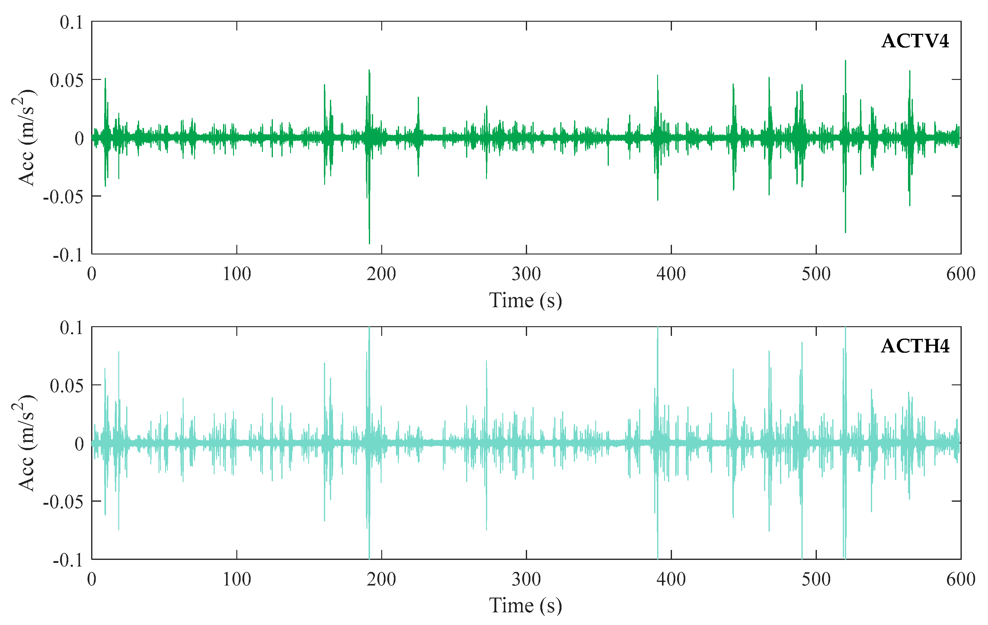
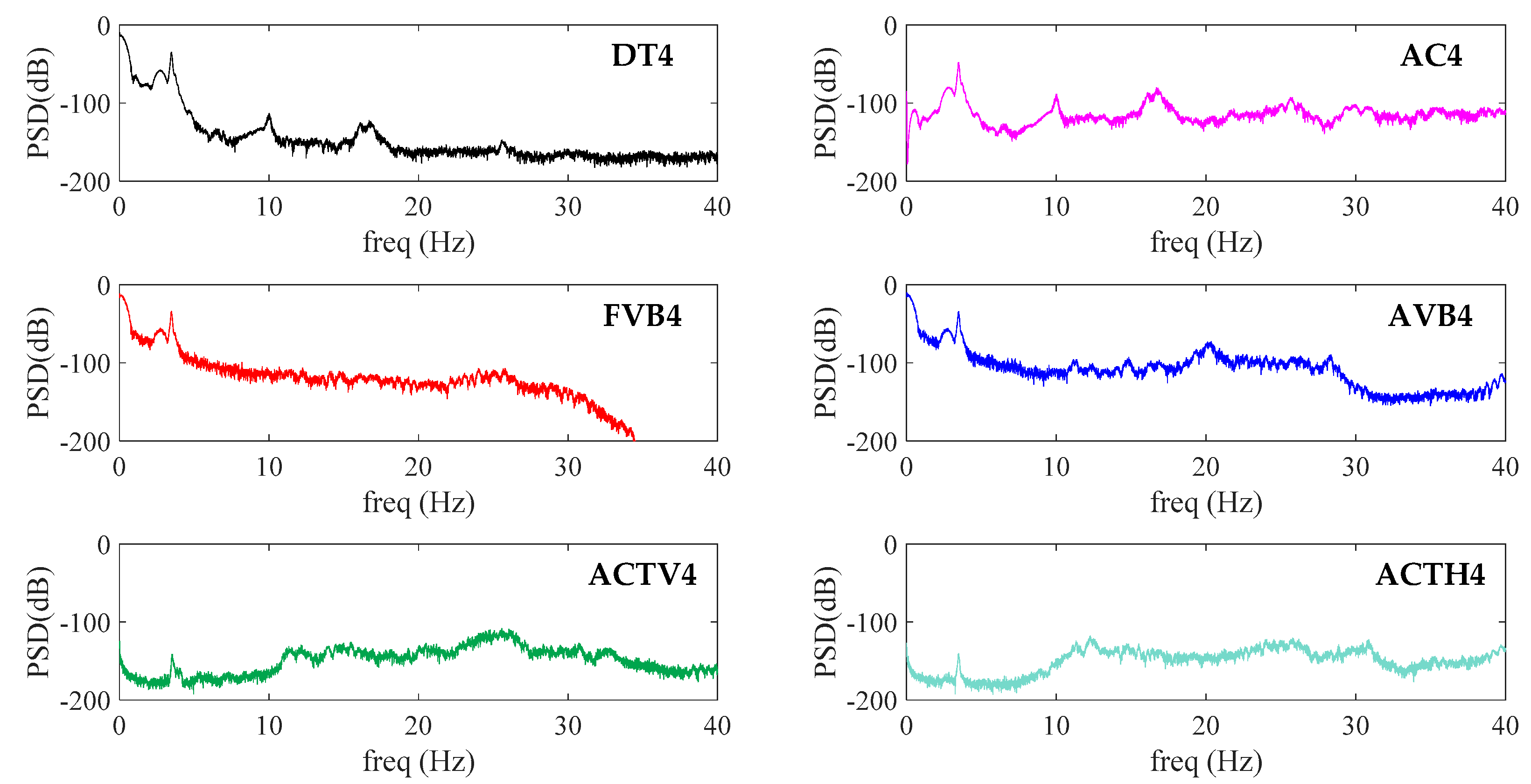
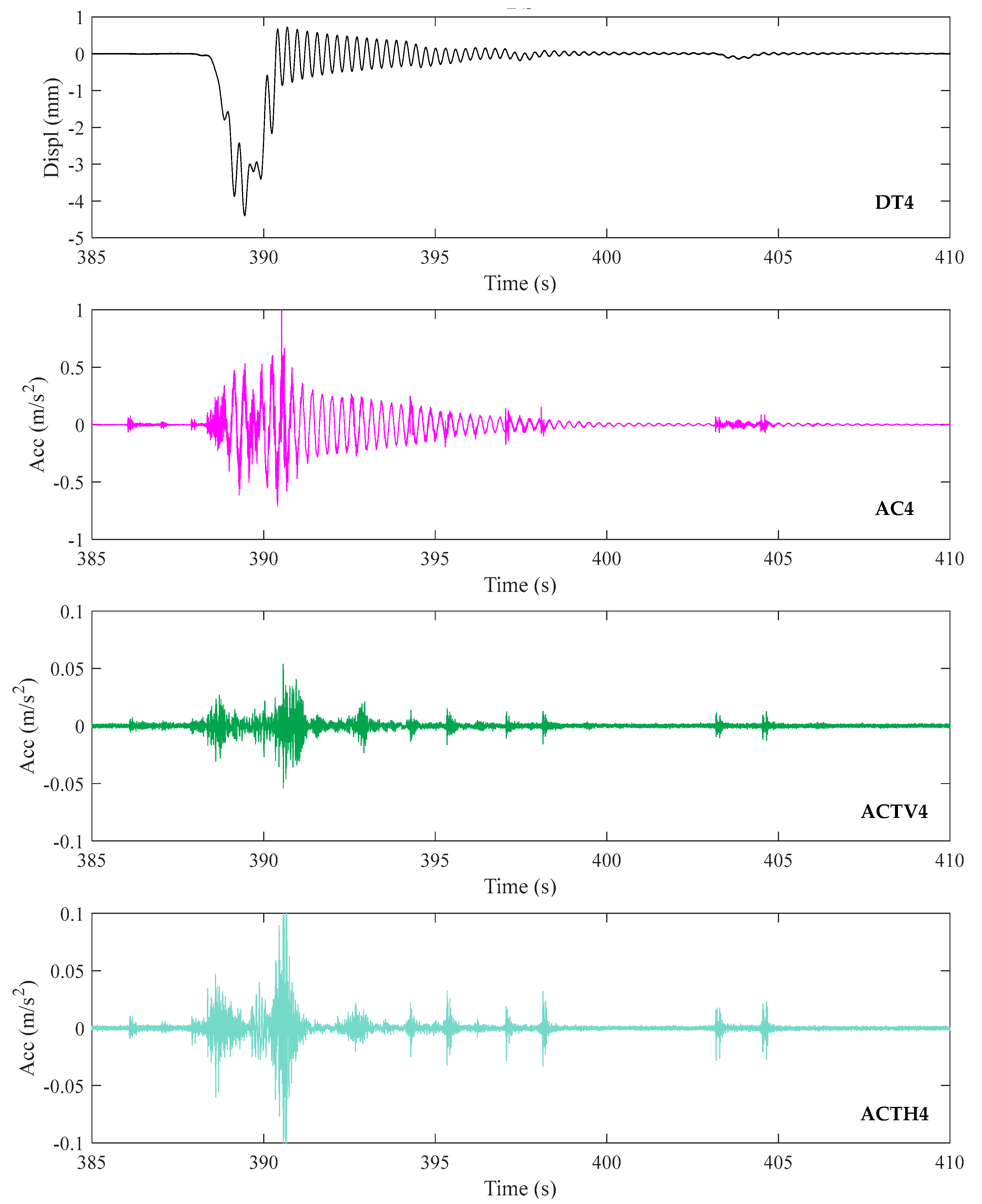
4.3. Analysis of Measured Accelerations

The signals of the accelerometer at midspan (AC) and the displacement recordings (DT, AVB, and FVB) were processed to compute the frequency of the first vertical mode of the monitored span. The obtained results (Table 6) show differences basically negligible in the frequencies determined from the measurements DT, AVB, and FVB with respect to AC, assumed as the reference value. Accordingly, the video cameras provided estimations of the first modal frequency equivalent to those obtained from the contact sensors, confirming the results already obtained for other bridge typologies [1,2,3,4].
To gain more insight into the frequency contents of DT, AVB, FVB, AC, ACTV, and ACTH, the Power Spectral Density (PSD) is shown for the fourth acquisition (Figure 22). It is observed that only AC and DT permit to recognise the subsequent two modal frequencies. It is also noted that the video cameras are affected by distinct noise above 10 Hz, more pronounced in camera A. Given that the PSDs of the accelerometers installed at the head of the tripod supporting video camera F are more pronounced in the frequency range between 12 and 32 Hz, it can be deduced that the noise in the readings of the cameras originates from the ground vibrations induced by the vehicular traffic on the bridge, filtered by the tripod and transmitted to the video camera. This noise has a frequency content outside the range of the first vibration mode of the bridge being monitored. Nevertheless, it also has a negative influence (although limited) on the accuracy of the peak displacement estimates because of the high-frequency spikes, as already observed.
The relations between the vehicular traffic and the noise in the displacement data extracted from the video cameras are further documented by the measurements presented in Figure 23, where the concurring vertical deflection, midspan deck acceleration, and accelerations on the tripod are shown when a heavy vehicle travels along the bridge. The accelerations in the tripod clearly testify the propagation of the traffic vibrations from the bridge to the ground, and hence in the tripod, as the main source of noise in the video cameras. At this regard, it is important to remark that very small movements of the camera can have an impact on the accuracy of displacement measurements if they induce rotations of the optical axis in the vertical plane. In fact, small rotations are amplified into non-negligible displacements of the camera with respect to the target, especially in the case of a lens with a long focal length and targets far from the camera, as is the case in this study and more in general when vision-based monitoring is adopted. Although the tripod supporting camera A was not equipped with accelerometers or other sensors (due to its smaller head with no space for instruments other than the video camera), the difference in mass (3.25 kg for the tripod of camera A versus 8.40 kg for the tripod of camera B with the added accelerometers) and geometry (larger legs and much larger head) allows to realistically assume a less stable condition for camera A with respect to camera F, adducing this as the main source of the previously observed differences between measurements AVB and FVB.
While the largest vibrations occur when the vehicle runs along the monitored span, there are also acceleration peaks when the midspan deflection is basically zero. This is a consequence of the impact of the vehicle on the expansion joints when entering the bridge, moving from one span to the other, and finally leaving the bridge. Accordingly, if the accelerations on the tripod over the entire 10 min acquisition window are considered, a larger number of peaks with respect to the deflection peaks can be counted, as exemplified in Figure 24 for the fourth acquisition window.

5. Discussion

The presented experimental study adopted two identical video cameras with different settings and installed on two different tripods (one of them equipped with two accelerometers) to monitor the midspan deflections of a medium-span post-tensioned concrete bridge under vehicular traffic. While the many applications of vision-based monitoring of bridges can be found in the literature, very few involved the considered structural typology, expected to be a more demanding test as compared to steel bridges and footbridges used in previous studies. The adopted hardware is simple and cost-effective; the implemented software is based on available computer-vision algorithms that require the installation of artificial targets in the points of the structure to be monitored. Given that no indications could be found in the literature for the choice of a proper target, a simple target design was proposed in this work to provide accuracy and efficiency in the detection of displacements, straightforward camera calibration procedures, and support for the selection of the region of interest (ROI) and template, whose movements within the ROI are tracked during monitoring.
Tests were conducted in a three-span post-tensioned concrete bridge under regular vehicular traffic, selected as it was possible to install a displacement transducer at the midspan of the first span to have a reference measure of the vertical deflection. The two cameras with their tripods were positioned on the ground under the bridge deck, close to the abutment and pointing at the target installed at the midspan, with the optical axis substantially parallel to the bridge axis. In this way, the cameras are in a position protected from rain and direct sunlight that might also be considered for long-term monitoring. Besides these major benefits, the adopted camera position gave two issues: illumination of the targets was insufficient, and the cameras were affected by vibrations transmitted through abutments and piers by the vehicles driving along the bridge. The first problem was solved using a lamp; the second problem was strongly reduced with the adoption of a low-pass filter. Nevertheless, the frequency content of the noise transmitted by the tripod to the cameras was not superimposed with the first natural frequency of the bridge deck; thus, it gave a negative impact mostly on the recordings of the transient response while the estimation of the peak displacements showed limited differences with respect to the reference measures by the contact sensor.
Based on the obtained results during the experimental tests presented in this article, the following remarks are made:
  • Cost-effective hardware (industrial camera, lens, artificial targets) together with software based on an upsampling cross-correlation (UCC) template matching algorithm can deliver accurate real-time measurements of the deflections of medium-span post-tensioned concrete bridges under vehicular traffic as well as precise estimations of their first mode frequency.
  • A simple method was proposed for the design of artificial targets based on just one design parameter (which defines both its global and local geometry) determined as a function of the distance between the camera and the target, the focal length of the adopted lens, and the pixel dimension of the camera sensor.
  • The proposed artificial target, in addition to its main function to serve as a high-contrast surface for the UCC template matching algorithm, was also conceived to allow a very simple camera calibration and to facilitate the selection of the region of interest (ROI) and the template within the ROI. This contributes to standardise the camera setting procedures for the benefit of measure replicability and ease of use.
  • Camera and software settings were varied to understand their effects on the quality of the measurements: one parameter influencing the time resolution, i.e., image acquisition frequency indicated by the acquired frames per second (FPS); three parameters influencing the displacement resolution, i.e., target size, focal length of the adopted lens, and upsampling factor in the UCC template matching algorithm.
  • Increasing FPS was expected to increase the quality of the measurements under dynamic loading. This was not the case due to high frequency noise introduced by the vibrations in the tripod. Thus, no clear benefits were obtained by increasing FPS in the range 30 to 240. This deduction is supposed to change if mechanical solutions to reduce noise will be implemented.
  • Changes in the parameters influencing the displacement resolution were made within the optimal range of the application of the proposed target design. No major benefit was clearly identified in lowering the minimum displacement that could be theoretically measured. However, the considered minimum displacement values were much lower that the peak displacements that were evaluated and lower than the noise induced by the vibrations in the tripod.
  • The differences in selecting the ROI and template as well as the differences in the computation of the pixel counts for camera calibration (one single measure or average of four measures), within the guide of the adopted artificial target, had no noticeable effects on the measurements.
  • The previous two points (no influence of parameters defining displacement resolution within the range imposed by the used target, camera calibration, ROI and template selection) show the effectiveness of the proposed target design in enforcing the replicability of the measurements in vision-based monitoring.
  • The geometric relations derived between the target size and distance, lens focal length, and pixel size of the camera sensor, can also be used to provide indications on the suitability of a given hardware setting or selecting the most appropriate hardware among those available.
  • Possible future developments of vision-based monitoring of post-tensioned concrete bridges are expected to deal with the identified critical aspects: illuminance of the target and vibration limitation of the video cameras.
  • Targets might be improved using highly reflective materials to avoid or reduce the use of lamps, or efficient and cost-effective retro-illuminated solutions.
  • Ways to limit the negative effects of vibrations transmitted to the video camera could be developed using different perspectives: mechanical devices (for example, decoupling connections or tuned tripods) or software algorithms (noise cancellation based on multi-point image tracking with the inclusion of stationary points).
  • A vision-based system, as the one here adopted, relaying on real-time image processing for the extraction of displacement time histories without the need to store large memory-consuming video footages, might be suitable for longer monitoring campaigns or permanent monitoring. However, pilot applications and relevant studies are inevitably required to evaluate the long-term performance of a vision-based system and how night-and-day as well as seasonal changing light conditions can be conveniently handled.

6. Conclusions

This experimental study was focused on the application of a simple and cost-effective vision-based structural monitoring system to a medium-span, post-tensioned, simply supported concrete bridge, a very common typology in many road networks. The objective was the investigation of the quality of the results that can be obtained, understanding the role and influence on the accuracy of the displacement measurements of various parameters relevant to the hardware settings, target geometry, and surrounding environment. Specific interest focused on highlighting possible difficulties and providing practical recommendations to achieve optimal results. The adopted monitoring system was shown to be a very efficient solution for expedite monitoring of the dynamic response of bridges under vehicular traffic, given that few operations are required in its installation, limited to target placement and video camera setup. The proposed target design allowed for simple camera calibration procedures and provided consistent results regardless of the adopted hardware settings, obtaining substantial equivalence of midspan deflection as compared to the reference contact sensor. In addition, very accurate estimates of the first modal frequency of the bridge deck were obtained as compared to the reference accelerometer. Critical aspects were identified in the illumination of the target and in the negative influence of the noise induced by the vehicular traffic in the tripod supporting the video cameras.

Author Contributions

Conceptualization, A.Z. and F.M.; methodology, A.Z., F.M., M.M. and A.D.; software, A.Z., F.M. and M.M.; validation, A.Z., F.M. and M.M.; formal analysis, A.Z., F.M. and M.M.; investigation, A.Z., F.M. and M.M.; resources, A.D.; data curation, A.Z., F.M. and M.M.; writing—original draft preparation, A.Z. and F.M.; writing—review and editing, A.Z, F.M., M.M. and A.D.; visualization, A.Z., F.M. and M.M.; supervision, A.Z. and A.D.; project administration, A.D.; funding acquisition, A.D. All authors have read and agreed to the published version of the manuscript.

Funding

This research was supported by FABRE “Research consortium for the evaluation and monitoring of bridges, viaducts, and other structures” (https://www.consorziofabre.it/).

Data Availability Statement

The data presented in this study are available on request from the corresponding author. The data are not publicly available due to restrictions imposed by the owner of the bridge.

Acknowledgments

The authors acknowledge ANAS Marche for providing them the opportunity to perform the tests in the case study bridge described in this work. The economic support provided by the FABRE Consortium for the contact and contactless structural monitoring systems adopted in this study is gratefully recognized.

Conflicts of Interest

The authors declare no conflict of interest.

References

  1. Feng, D.; Feng, M.Q. Computer vision for SHM of civil infrastructure: From dynamic response measurement to damage detection—A review. Eng. Struct. 2018, 156, 105–117. [Google Scholar] [CrossRef]
  2. Dong, C.Z.; Catbas, F.N. A review of computer vision–based structural health monitoring at local and global levels. Struct. Health Monit. 2021, 20, 692–743. [Google Scholar] [CrossRef]
  3. Feng, D.; Feng, M.Q. Computer Vision for Structural Dynamics and Health Monitoring, 1st ed.; Wiley: Hoboken, NJ, USA, 2021; pp. 1–234. [Google Scholar]
  4. Zona, A. Vision-based vibration monitoring of structures and infrastructures: An overview of recent applications. Infrastructures 2021, 6, 4. [Google Scholar] [CrossRef]
  5. Luo, K.; Kong, X.; Zhang, J.; Hu, J.; Li, J.; Tang, H. Computer vision-based bridge inspection and monitoring: A review. Sensors 2023, 23, 7863. [Google Scholar] [CrossRef]
  6. Bhowmick, S.; Nagarajaiah, S. Identification of full-field dynamic modes using continuous displacement response estimated from vibrating edge video. J. Sound Vib. 2020, 489, 115657. [Google Scholar] [CrossRef]
  7. Aliansyah, Z.; Shimasaki, K.; Senoo, T.; Ishii, I.; Umemoto, S. Single-camera-based bridge structural displacement measurement with traffic counting. Sensors 2021, 21, 4517. [Google Scholar] [CrossRef]
  8. Kromanis, R.; Kripakaran, P. A multiple camera position approach for accurate displacement measurement using computer vision. J. Civ. Struct. Health Monit. 2021, 11, 661–678. [Google Scholar] [CrossRef]
  9. Lydon, D.; Lydon, M.; Kromanis, R.; Dong, C.-Z.; Catbas, N.; Taylor, S. Bridge damage detection approach using a roving camera technique. Sensors 2021, 21, 1246. [Google Scholar] [CrossRef]
  10. Obiechefu, C.B.; Kromanis, R. Damage detection techniques for structural health monitoring of bridges from computer vision derived parameters. Struct. Monit. Maint. 2021, 8, 91–110. [Google Scholar] [CrossRef]
  11. Voordijk, H.; Kromanis, R. Technological mediation and civil structure condition assessment: The case of vision-based systems. Civ. Eng. Environ. Syst. 2022, 39, 48–65. [Google Scholar] [CrossRef]
  12. Lydon, D.; Kromanis, R.; Lydon, M.; Early, J.; Taylor, S. Use of a roving computer vision system to compare anomaly detection techniques for health monitoring of bridges. J. Civ. Struct. Health Monit. 2022, 12, 1299–1316. [Google Scholar] [CrossRef]
  13. Nie, G.-Y.; Bodda, S.S.; Sandhu, H.K.; Han, K.; Gupta, A. Computer-vision-based vibration tracking using a digital camera: A sparse-optical-flow-based target tracking method. Sensors 2022, 22, 6869. [Google Scholar] [CrossRef] [PubMed]
  14. Bocian, M.; Nikitas, N.; Kalybek, M.; Kuzawa, M.; Hawryszków, P.; Bień, J.; Onysyk, J.; Biliszczuk, J. Dynamic performance verification of the Rędziński Bridge using portable camera-based vibration monitoring systems. Archiv. Civ. Mech. Eng. 2023, 23, 40. [Google Scholar] [CrossRef]
  15. Shajihan, S.A.V.; Hoang, T.; Mechitov, K.; Spencer, B.F. Wireless SmartVision system for synchronized displacement monitoring of railroad bridges. Comput. Aided Civ. Inf. 2022, 37, 1070–1088. [Google Scholar] [CrossRef]
  16. Ghyabi, M.; Timber, L.C.; Jahangiri, G.; Lattanzi, D.; Shenton, H.W., III; Chajes, M.J.; Head, M.H. Vision-based measurements to quantify bridge deformations. J. Bridge Eng. 2023, 28, 05022010. [Google Scholar] [CrossRef]
  17. Shao, Y.; Li, L.; Li, J.; Li, Q.; An, S.; Hao, H. Monocular vision based 3D vibration displacement measurement for civil engineering structures. Eng. Struct. 2023, 293, 116661. [Google Scholar] [CrossRef]
  18. Han, Y.; Wu, G.; Feng, D. Structural modal identification using a portable laser-and-camera measurement system. Measurement 2023, 214, 112768. [Google Scholar] [CrossRef]
  19. Rajaei, S.; Hogsett, G.; Chapagain, B.; Banjade, S.; Ghannoum, W. Vision-based large-field measurements of bridge deformations. J. Bridge Eng. 2023, 28, 04023075. [Google Scholar] [CrossRef]
  20. Yin, Y.; Yu, Q.; Hu, B.; Zhang, Y.; Chen, W.; Liu, X.; Ding, X. A vision monitoring system for multipoint deflection of large-span bridge based on camera networking. Comput. Aided Civ. Inf. 2023, 38, 1879–1891. [Google Scholar] [CrossRef]
  21. Dong, C.; Bas, S.; Catbas, F.N. Applications of computer vision-based structural monitoring on long-span bridges in Turkey. Sensors 2023, 23, 8161. [Google Scholar] [CrossRef]
  22. Choi, J.; Ma, Z.; Kim, K.; Sohn, H. Continuous structural displacement monitoring using accelerometer, vision, and infrared (IR) cameras. Sensors 2023, 23, 5241. [Google Scholar] [CrossRef] [PubMed]
  23. Luan, L.; Liu, Y.; Sun, H. Extracting high-precision full-field displacement from videos via pixel matching and optical flow. J. Sound Vib. 2023, 565, 117904. [Google Scholar] [CrossRef]
  24. Gentile, C.; Bernardini, G. An interferometric radar for noncontact measurement of deflections on civil engineering structures: Laboratory and full-scale tests. Struct. Infrastruct. Eng. 2010, 6, 521–534. [Google Scholar] [CrossRef]
  25. Negulescu, C.; Luzi, G.; Crosetto, M.; Raucoules, D.; Roullé, A.; Monfort, D.; Pujades, L.; Colas, B.; Dewez, T. Comparison of seismometer and radar measurements for the modal identification of civil engineering structures. Eng. Struct. 2013, 51, 10–22. [Google Scholar] [CrossRef]
  26. Gonzalez-Drigo, R.; Cabrera, E.; Luzi, G.; Pujades, L.G.; Vargas-Alzate, Y.F.; Avila-Haro, J. Assessment of post-earthquake damaged building with interferometric real aperture radar. Remote Sens. 2019, 11, 2830. [Google Scholar] [CrossRef]
  27. Michel, C.; Keller, S. Advancing ground-based radar processing for bridge infrastructure monitoring. Sensors 2021, 21, 2172. [Google Scholar] [CrossRef]
  28. Xia, H.; De Roeck, G.; Zhang, N.; Maeck, J. Experimental analysis of a high-speed railway bridge under Thalys trains. J. Sound Vib. 2003, 268, 103–113. [Google Scholar] [CrossRef]
  29. Nassif, H.H.; Gindy, M.; Davis, J. Comparison of laser Doppler vibrometer with contact sensors for monitoring bridge deflection and vibration. NDT E Int. 2005, 38, 213–218. [Google Scholar] [CrossRef]
  30. Garg, P.; Moreu, F.; Ozdagli, A.; Taha, M.R.; Mascareñas, D. Noncontact dynamic displacement measurement of structures using a moving laser doppler vibrometer. J. Bridge Eng. 2019, 24, 04019089. [Google Scholar] [CrossRef]
  31. Yu, W.; Nishio, M. Multilevel structural components detection and segmentation toward computer vision-based bridge inspection. Sensors 2022, 22, 3502. [Google Scholar] [CrossRef]
  32. Cardellicchio, A.; Ruggieri, S.; Nettis, A.; Renò, V.; Uva, G. Physical interpretation of machine learning-based recognition of defects for the risk management of existing bridge heritage. Eng. Fail. Anal. 2023, 149, 107237. [Google Scholar] [CrossRef]
  33. Wu, Z.; Tang, Y.; Hong, B.; Liang, B.; Liu, Y. Enhanced precision in dam crack width measurement: Leveraging advanced lightweight network identification for pixel-level accuracy. Int. J. Intell. Syst. 2023, 2023, 9940881. [Google Scholar] [CrossRef]
  34. Tang, Y.; Huang, Z.; Chen, Z.; Chen, M.; Zhou, H.; Zhang, H.; Sun, J. Novel visual crack width measurement based on backbone double-scale features for improved detection automation. Eng. Struct. 2023, 274, 115158. [Google Scholar] [CrossRef]
  35. Guizar-Sicairos, M.; Thurman, S.T.; Fienup, J.R. Efficient subpixel image registration algorithms. Opt. Lett. 2008, 33, 156–158. [Google Scholar] [CrossRef]
  36. Karybali, I.G.; Psarakis, E.Z.; Berberidis, K.; Evangelidis, G.D. An efficient spatial domain technique for subpixel image registration. Signal Process. Image Commun. 2008, 23, 711–724. [Google Scholar] [CrossRef]
  37. Feng, D.; Feng, M.Q.; Ozer, E.; Fukuda, Y. A vision-based sensor for noncontact structural displacement measurement. Sensors 2015, 15, 16557–16575. [Google Scholar] [CrossRef]
  38. Mas, D.; Perez, J.; Ferrer, B.; Espinosa, J. Realistic limits for subpixel movement detection. Appl. Opt. 2016, 55, 4974–4979. [Google Scholar] [CrossRef]
  39. Antoš, J.; Nežerka, V.; Somr, M. Real-time optical measurement of displacements using subpixel image registration. EXP Tech 2019, 43, 315–323. [Google Scholar] [CrossRef]
  40. Pinto, P.E.; Franchin, P. Issues in the upgrade of Italian highway structures. J. Earthq. Eng. 2010, 14, 1221–1252. [Google Scholar] [CrossRef]
  41. Gkoumas, K.; Marques Dos Santos, F.L.; van Balen, M.; Tsakalidis, A.; Ortega Hortelano, A.; Grosso, M.; Haq, G.; Pekár, F. Research and Innovation in Bridge Maintenance, Inspection and Monitoring—A European Perspective Based on the Transport Research and Innovation Monitoring and Information System (TRIMIS); EUR 29650 EN; Publications Office of the European Union: Luxembourg City, Luxembourg, 2019. [Google Scholar] [CrossRef]
  42. Neves, A.C.; Leander, J.; González, I.; Karoumi, R. An approach to decision-making analysis for implementation of structural health monitoring in bridges. Struct. Control Health Monit. 2019, 26, e2352. [Google Scholar] [CrossRef]
  43. An, Y.; Chatzi, E.; Sim, S.H.; Laflamme, S.; Blachowski, B.; Ou, J. Recent progress and future trends on damage identification methods for bridge structures. Struct. Control Health Monit. 2019, 26, e2416. [Google Scholar] [CrossRef]
  44. Ercolessi, S.; Fabbrocino, G.; Rainieri, C. Indirect measurements of bridge vibrations as an experimental tool supporting periodic inspections. Infrastructures 2021, 6, 39. [Google Scholar] [CrossRef]
  45. Rainieri, C.; Notarangelo, M.A.; Fabbrocino, G. Experiences of dynamic identification and monitoring of bridges in serviceability conditions and after hazardous events. Infrastructures 2020, 5, 86. [Google Scholar] [CrossRef]
  46. D’Alessandro, A.; Birgin, H.B.; Cerni, G.; Ubertini, F. Smart infrastructure monitoring through self-sensing composite sensors and systems: A study on smart concrete sensors with varying carbon-based filler. Infrastructures 2022, 7, 48. [Google Scholar] [CrossRef]
  47. D’Angelo, M.; Menghini, A.; Borlenghi, P.; Bernardini, L.; Benedetti, L.; Ballio, F.; Belloli, M.; Gentile, C. Hydraulic safety evaluation and dynamic investigations of Baghetto Bridge in Italy. Infrastructures 2022, 7, 53. [Google Scholar] [CrossRef]
  48. Nicoletti, V.; Martini, R.; Carbonari, S.; Gara, F. Operational modal analysis as a support for the development of digital twin models of bridges. Infrastructures 2023, 8, 24. [Google Scholar] [CrossRef]
  49. Kim, H.-J.; Seong, Y.-H.; Han, J.-W.; Kwon, S.-H.; Kim, C.-Y. Demonstrating the test procedure for preventive maintenance of aging concrete bridges. Infrastructures 2023, 8, 54. [Google Scholar] [CrossRef]
  50. Natali, A.; Cosentino, A.; Morelli, F.; Salvatore, W. Multilevel approach for management of existing bridges: Critical analysis and application of the Italian Guidelines with the new operating instructions. Infrastructures 2023, 8, 70. [Google Scholar] [CrossRef]
  51. Mathworks MATLAB Version 2023a; The MathWorks Inc.: Natick, MA, USA. 2023. Available online: https://www.mathworks.com (accessed on 20 September 2023).
  52. Mathworks MATLAB Computer Vision Toolbox. Available online: https://mathworks.com/products/computer-vision.html (accessed on 20 September 2023).
  53. Mathworks MATLAB Image Acquisition Toolbox Support Package for GenICam. Interface MATLAB Central File Exchange. Available online: https://mathworks.com/matlabcentral/fileexchange/45180-image-acquisition-toolbox-support-package-for-genicam-interface (accessed on 20 September 2023).
  54. Guizar, M. Efficient Subpixel Image Registration by Cross-Correlation. MATLAB Central File Exchange. Available online: https://www.mathworks.com/matlabcentral/fileexchange/18401-efficient-subpixel-image-registration-by-cross-correlation (accessed on 20 September 2023).
  55. Teledyne FLIR Blackfly S BFS-U3-23S3 Specifications and Frame Rates. Available online: http://softwareservices.flir.com/BFS-U3-23S3/latest/Model/spec.html (accessed on 20 September 2023).
  56. Teledyne FLIR Blackfly S BFS-U3-23S3 Imaging Performance. Available online: http://softwareservices.flir.com/BFS-U3-23S3/latest/EMVA/EMVA.html (accessed on 20 September 2023).
  57. Teledyne FLIR Blackfly S BFS-U3-23S3 Readout Method. Available online: http://softwareservices.flir.com/BFS-U3-23S3/latest/40-Installation/Readout.htm (accessed on 20 September 2023).
  58. Yang, Y.B.; Yau, J.D.; Wu, Y.S. Vehicle–Bridge Interaction Dynamics with Applications to High-Speed Railways; World Scientific Publishing Co.: Singapore, 2004; pp. 1–530. [Google Scholar]
  59. Yang, Y.B.; Lin, C.W. Vehicle–bridge interaction dynamics and potential applications. J. Sound Vib. 2005, 284, 205–226. [Google Scholar] [CrossRef]
  60. Orfanidis, S.J. Optimum Signal Processing: An Introduction, 2nd ed.; Prentice-Hall: Englewood Cliffs, NJ, USA, 1996; pp. 1–377. [Google Scholar]
Figure 1. Main technical specifications, characteristics, and conditions influencing the performance of a vision-based monitoring system.
Infrastructures 08 00152 g001
Figure 2. Exemplification of the flowchart of the adopted video processing algorithm.
Infrastructures 08 00152 g002
Figure 3. Geometric parameters relevant to SF.
Infrastructures 08 00152 g003
Figure 4. An example of the proposed target design (left) and suggested definition of the ROI and template within the target (right).
Infrastructures 08 00152 g004
Figure 5. Examples of the proposed target as seen using different pixel resolutions.
Infrastructures 08 00152 g005
Figure 6. Lower and upper bounds recommended for the proposed target dimensions for lens focal lengths f = 50 mm and f = 100 mm (dpixel = 3.45 µm). Exemplification of the application range of targets with dimensions 10t = 50 mm and 10t = 100 mm.
Infrastructures 08 00152 g006
Figure 7. Aerial view of the case study bridge on the day of testing.
Infrastructures 08 00152 g007
Figure 8. Lateral view of the case study bridge on the day of testing.
Infrastructures 08 00152 g008
Figure 9. Schematic view of the monitored span of the bridge with indication of the adopted sensors.
Infrastructures 08 00152 g009
Figure 10. Video cameras during an acquisition phase and targets installed at midspan, in addition to a displacement transducer and accelerometers.
Infrastructures 08 00152 g010
Figure 11. Comparisons between DT4, AVB4 (FPS 120), and FVB4 (FPS 60) in the entire acquisition window. The red box highlights the portion in the close-up of the next figure.
Infrastructures 08 00152 g011
Figure 12. Comparisons between DT4, AVB4 (FPS 120), and FVB4 (FPS 60) in the tract of the fourth window corresponding to the passage of the third heavy vehicle.
Infrastructures 08 00152 g012
Figure 13. Comparisons between DT5, AVB5 (FPS 240), and FVB5 (FPS 120) in the entire acquisition window. The red box highlights the portion in the close-up of the next figure.
Infrastructures 08 00152 g013
Figure 14. Comparisons between DT5, AVB5 (FPS 240), and FVB5 (FPS 120) in the tract of the fifth window corresponding to the passage of the second and third closely spaced heavy vehicles.
Infrastructures 08 00152 g014
Figure 15. Comparisons between DT6, AVB6 (f = 100 mm), and FVB6 (f = 50 mm) in the entire acquisition window. The red box highlights the portion in the close-up of the next figure.
Infrastructures 08 00152 g015
Figure 16. Comparisons between DT6, AVB6 (f = 100 mm), and FVB6 (f = 50 mm) in the tract of the sixth window corresponding to the passage of the eighth heavy vehicle.
Infrastructures 08 00152 g016
Figure 17. Comparisons between DT4, AVB4 (low-pass filter), and FVB4 (raw signal) in the tract of the fourth window corresponding to the passage of the third heavy vehicle.
Infrastructures 08 00152 g017
Figure 18. Comparisons between DT5, AVB5 (LPF), and FVB5 (raw signal) in the tract of the fifth window corresponding to the passage of the second and third closely spaced heavy vehicles.
Infrastructures 08 00152 g018
Figure 19. Comparisons between DT5, AVB5 (LPF), and FVB5 (LPF) in the tract of the fifth window corresponding to the passage of the second and third closely spaced heavy vehicles.
Infrastructures 08 00152 g019
Figure 20. Comparisons between DT6, AVB6 (LPF), and FVB6 (raw signal) in the tract of the sixth window corresponding to the passage of the eighth heavy vehicle.
Infrastructures 08 00152 g020
Figure 21. Absolute differences in the displacements for the original and filtered measurements obtained from the video cameras with respect to the contact sensor.
Infrastructures 08 00152 g021
Figure 22. Power Spectral Density (PSD) in the fourth 10 min window from the displacement transducer (DT), the accelerometer at midspan (AC), the two video cameras (AVB and FVB), and the accelerometers on the tripod of camera F (vertical ACTV and horizontal ACTH directions).
Infrastructures 08 00152 g022
Figure 23. Trend of the accelerations on the bridge deck and at the top of the tripod of camera F at the occurrence of a deflection peak (DT4, AC4, ACTV4, ACTH4) in the window corresponding to the passage of the third heavy vehicle in the fourth acquisition window.
Infrastructures 08 00152 g023
Figure 24. Vertical (ACTV) and horizontal (ACTH) accelerations at the top of the tripod supporting camera F in the fourth 10-min window.
Infrastructures 08 00152 g024
Table 1. Adopted vision-based monitoring hardware.
ComponentModelMain Technical Specifications
Video cameraTeledyne FLIR BLACKFLY S BFS-U3-23S3M-CSensor: Sony IMX392 CMOS 1/2.3″
Pixel size: 3.45 µm
Max resolution: 1920 × 1200 (2.3 M pixels)
Readout method: Global shutter
Chroma: Monochrome
Exposure range: 6.0 μs to 30.0 s
Max FPS at full resolution: 163
Max FPS at 640 × 480 resolution: 392
Max FPS at 320 × 240 resolution: 717
Mass: 36 g
LensTamron 23FM50SPFocal length: 50 mm
Max aperture: F2.8
Distortion: <0.01%
Focus range: 0.2 m–∞
Field angle (H × V): 7.6 × 4.8°
Mass: 117 g
Kowa LM100JC1MSFocal length: 100 mm
Max aperture: F2.8
Distortion: <0.05%
Focus range: 2.0 m–∞
Field angle (H × V): 3.8 × 2.4°
Mass: 145 g
Table 2. Settings of the vision-based monitoring acquisitions.
Start TimeMeasuref (mm)FPS10t (mm)ROI SizePixel SearchSF (mm)
12:15AVB110012050129 × 128 250.4254
FVB110012050183 × 178250.4184
12:30AVB210012050115 × 114 190.4237
FVB210012050174 × 170200.4155
12:45AVB310012050122 × 124230.4247
FVB31003050170 × 167200.4218
13:05AVB410012050123 × 122230.4256
FVB41006050168 × 166200.4173
13:30AVB510024050111 × 110180.4259
FVB510012050160 × 156150.4172
13:55AVB610012050124 × 122 230.4256
FVB6501205085 × 83100.8429
16:00FVB750120100145 × 145150.8416
Table 3. Environmental conditions below the bridge during the tests (20 July 2023).
TimeTemperature (°C)Relative Humidity (%)
11:0031.645.9
12:0031.940.4
13:0032.537.9
14:0032.538.3
15:0032.846.3
16:0032.256.2
Table 4. Comparisons of displacement measures.
MeasureDisp. Res.
Rdisp (mm)
Disp. Range
dmax (mm)
Heavy
Vehicles
Max Disp.
(mm)
Max Disp.
Diff. (mm)
Max Disp.
Diff. (%)
Mean Abs
Diff. (mm)
Std Abs
Diff. (mm)
DT11.19 × 10−5100 2.533
AVB10.00425410.63542.6620.1295.100.0910.045
FVB10.00836810.460 2.5840.0512.000.0190.022
DT21.19 × 10−5100 3.433
AVB20.0042378.050333.5860.1534.440.1060.074
FVB20.0041558.3100 3.4680.0351.010.0450.035
DT31.19 × 10−5100 3.778
AVB30.0042479.7681243.8730.0952.510.1300.066
FVB30.0042188.4360 3.8440.0661.750.0480.024
DT41.19 × 10−5100 4.712
AVB40.0042569.788854.9440.2324.930.0890.095
FVB40.0041738.3460 4.7120.0000.000.0200.019
DT51.19 × 10−5100 4.608
AVB50.0042597.666294.7320.1242.710.1570.037
FVB50.0041726.2580 4.6170.0090.210.0480.043
DT61.19 × 10−5100 4.640
AVB60.0042569.7888124.8300.1904.100.1590.080
FVB60.0084298.4290 4.6700.0300.650.0440.039
DT71.19 × 10−5100134.766
FVB70.00841612.6244.674−0.092−1.930.0610.055
Table 5. Comparisons of displacement measures with AVB and FVB filtered using a 15 Hz LPF.
MeasureMax Disp.
(mm)
Max Disp.
Diff. (mm)
Max Disp.
Diff. (%)
Mean Abs
Diff. (mm)
Std Abs
Diff. (mm)
DT12.533
AVB1 (LPF)2.5680.0351.360.0380.035
FVB1 (LPF)2.5780.0451.770.0180.018
DT23.433
AVB2 (LPF)3.5060.0732.100.0570.041
FVB2 (LPF)3.4580.0250.720.0390.032
DT33.778
AVB3 (LPF)3.8840.1062.810.0580.040
FVB3 (LPF)3.8440.0661.750.0470.024
DT44.712
AVB4 (LPF)4.8970.1853.920.0640.082
FVB4 (LPF)4.702−0.010−0.120.0210.019
DT54.608
AVB5 (LPF)4.7070.0992.150.0610.043
FVB5 (LPF)4.605−0.003−0.060.0490.043
DT64.640
AVB6 (LPF)4.7040.0641.390.0670.052
FVB6 (LPF)4.6490.0090.200.0360.036
DT74.766
FVB7 (LPF)4.674−0.092−1.940.0580.055
Table 6. Comparisons of the obtained 1st mode frequency from accelerometer at midspan (AC), displacement transducer (DT), and the two video cameras (AVB and FVB).
Acquisition WindowACDTAVBFVB
Freq. (Hz)Freq. (Hz)Diff. (%)Freq. (Hz)Diff. (%)Freq. (Hz)Diff. (%)
#13.483.480.003.480.003.480.00
#23.473.480.133.480.133.470.00
#33.453.45−0.133.45−0.133.45−0.13
#43.473.470.003.470.003.470.00
#53.483.480.003.480.003.480.00
#63.483.480.003.480.003.480.00
#73.473.470.13--3.470.13
Disclaimer/Publisher’s Note: The statements, opinions and data contained in all publications are solely those of the individual author(s) and contributor(s) and not of MDPI and/or the editor(s). MDPI and/or the editor(s) disclaim responsibility for any injury to people or property resulting from any ideas, methods, instructions or products referred to in the content.

