Urban Heat Island High Water-Vapor Feedback Estimates and Heatwave Issues: A Temperature Difference Approach to Feedback Assessments

Abstract

The goal of this paper is to provide an initial assessment of water-vapor feedback (WVF) in humid urban heat island (UHI) environments based on temperature difference data. To achieve this, a novel temperature difference WVF model was developed that can analyze global and UHI local temperature difference data. Specifically, the model was applied to a comparative temperature literature study of similar cities located in humid versus dry climates. The literature study found that the daytime UHI ΔT was observed to be 3.3 K higher in humid compared to dry climates when averaged over thirty-nine cities. Since the direct measurement of WVF in UHI areas could prove challenging due to variations in the temperature lapse rates from tall buildings, modeling provides an opportunity to make a preliminary assessment where measurements may be difficult. Thus, the results provide the first available UHI ΔT WVF model assessment. The preliminary results find local water-vapor feedback values for wet-biased cities of 3.1 Wm⁻²K⁻¹, 3.4 Wm⁻²K⁻¹, and 4 Wm⁻²K⁻¹ for 5 °C, 15 °C, and 30 °C UHI average temperatures, respectively. The temperature difference model could also be used to reproduce literature values. This capability helps to validate the model and its findings. Heatwave assessments are also discussed, as they are strongly affected by UHI water-vapor feedback and support the observation that humid regions amplify heat higher than UHIs in dry regions, exacerbating heatwave problems. Furthermore, recent studies have found that urbanization contributions to global warming more than previously anticipated. Therefore, cities in humid environments are likely larger contributors to such warming trends compared to cities in dry environments. These preliminary modeling results show concern for a strong local UHI water-vapor feedback issue for cities in humid environments, with results possibly over a factor of two higher than the global average. This assessment also indicates that albedo management would likely be an effective way to reduce the resulting WVF temperature increase.

1. Introduction

Observations of excess water vapor steaming off hot city roads and surfaces during precipitation are commonplace, especially in humid environments. This is a gross observation that is easy to detect during precipitation periods in UHIs. However, complex subtle warming feedback effects occur in wet environments, amplifying the UHI intensity compared to dry environments. A humidity effect, where UHI daytime wet vs. dry environmental temperature differences showed a strong increase in ∆T with an average of 3.3 K was observed in a 2014 study by Zhao et al. [1], which is detailed in Section 2. In this paper, a temperature difference WVF model (WVFM) is developed, and using the data in their study, preliminary wet-biased WVF UHI estimates are provided.

The cities selected in the Zhao et al. (2014) [1] study were based on precipitation amounts. In this paper, the observation of increased warming in humid cities is assumed to be due to water-vapor feedback, which is associated with cities having reduced cooling efficiencies. UHI convection cooling to the lower troposphere includes warm water-vapor air parcels and their re-radiation effect. If water-vapor feedback was not an issue, the opposite would occur, and cities in high precipitation regions would cool more than cities in dry regions. Furthermore, feedback causes an amplification that can occur from several mechanisms, as described below. The key requirement for WVF estimates is that they are derived using the constraints of the water-vapor feedback equation (see Section 2, Section 3 and Section 4). The ∆T WVFM meets these constraints and is reasonably robust, as it was also used to reproduce literature results (see Section 3.1).

Other authors have observed the exacerbation effects of humid environments, and in particular there has been work in the area on heatwaves (HWs). This is the main concern for UHIs since humid heat creates harsh adverse conditions that can impact health and death rates [2,3,4,5,6,7] and adverse economic issues [8,9]). Since 55% of the population now lives in cities, and this is expected to increase to near 70% by 2050 [10], heatwaves are a major concern that can be affected by UHI water-vapor feedback. Wang et al. (2021) [11] studied intensified humid heat events under global warming and found that that, “Humid heat events show intensifications to dry heat events with higher frequency, duration, and intensity”.

Empirical HW evidence exists for synergistic effects [12,13]. Liao et al. (2018) [13], in a study on HW exacerbation from UHIs in dry versus wet climates in China, also showed a strong synergistic heatwave effect that was observed both in duration and frequency. Liao also noted that “in wet climates, the increasing trends of HWs in urban areas are greater than those in rural areas, suggesting a positive contribution of urbanization to HW trends.”

Li et al. (2020) [14] showed that the summer mean wet bulb globe temperature (WBGT) has increased almost everywhere across China since 1961 as a result of human-induced climate change. Consequently, hot summers, as measured by the summer mean WBGT, are becoming more frequent and more conducive to heat stress. Hot summers, such as the hottest on record during 1961–2015 in western or eastern China, are now expected to occur once every 3 to 4 years. These hot WBGT summers have become more than 140 times as likely in eastern China and more than 1000 times as likely in western China in the present decade (the 2020s) as in the 1961–1990 baseline period.

Russo et al. (2017) [15] “found that the magnitude and apparent temperature peak of heatwaves, such as the ones observed in Chicago in 1995 and China in 2003, have been strongly amplified by humidity. Climate model projections suggest that the percentage of the area where heatwave magnitude and peaks are amplified by humidity increases with increasing warming levels.” The studied regions included the eastern U.S., similar to the work by Zhao et al. (2014) [1].

Other authors have studied heatwaves in various humid climates where water-vapor feedback is problematic. Li and Zeid (2013) [12] studied the Baltimore–Washington metropolitan humid areas and found “synergies between urban heat islands and heatwaves. That is, not only do HWs increase the ambient temperatures, but they also intensify the difference between urban and rural temperatures. As a result, the added heat stress in cities will be even higher than the sum of the background urban heat island effect and the heatwave effect.” In China, Knong et al. (2020) [16] found “the occurrence probability of human-perceived HW nearly doubled over the recent decades, of which urbanization and greenhouse gases contribute to 21.9% and 72.9% of the intensification of HWs, respectively”. Zou et al. (2021) [17], showed that “the UHI effect was significantly amplified during HWs.” In the very humid wet climate of Bangladesh, Dewan et al. (2021) found, “Results indicated that annual surface urban heat island intensity (SUHII) was greater in the larger cities of Dhaka and Chittagong than in the smaller cities. SUHII observed during the day was also greater than at night.” This supports Zhao et al.’s (2014) daytime observations, which are detailed in Section 2.

In general, these heatwave observations illustrate the importance of UHI water-vapor feedback and help qualitatively support Zhao et al.’s (2014) results (see Section 2 and Section 3) with the general conclusion that humid environments can significantly amplify UHI intensity.

The actual mechanism causing UHI daytime humid vs. dry environmental temperature differences may not be fully understood. Zhao et al. (2014) described the effect as “largely explained by variations in the efficiency with which urban and rural areas convect heat to the lower atmosphere. If urban areas are aerodynamically smoother than surrounding rural areas, urban heat dissipations are relatively less efficient, and urban warming occurs (and vice versa).”

In addition to convection cooling inefficiencies, it is also possible that water-vapor greenhouse gas (GHG) effects also contribute. This would increase long-wavelength downwelling in humid environments. Daytime air temperatures are also typically higher in UHIs. The specific humidity can increase (Fan et al. 2017) quickly due to warmer daytime UHI temperatures from impermeable surfaces in humid environments. Since warm air holds more water vapor and the environment is humid, it is not unreasonable to suspect that local water-vapor GHG also plays a role. Therefore, while the actual mechanism is not well understood, Zhao et al.’s observation may consist of a dual mechanism. Somewhat supportive is the work of Yang et al. (2017) [18] in eastern China (a humid environment in the summer) that found, “Overall, urbanization contributes to more than one-third of the increase of intensity of extreme heat events in the region, which is comparable to the contribution of greenhouse gases.”

Another interesting effect that reduces convection cooling efficiencies is temperature inversions. This effect is not well studied, so there are no data to support this possible increase in humid vs. dry environments, other than the fact that they reduce convection efficiency. One possible mechanism is that humid denser hot air parcels likely have lower convection cooling efficiencies in areas prone to daytime solar temperature inversions. This effect should be studied further in dry versus humid environments. For example, Bornstein (1968) [19] assessed temperature inversion in New York City and noted, “On mornings with relatively strong urban elevated inversion layers, the heat island extended to well over 500 m”. Without inversion layers, Bornstein noted the heat extended to about 300 m. Fast et al. (2005) [20] made measurements over Phoenix, Az., and noted “The peak UHI usually occurred around midnight; however, a strong UHI was frequently observed 2–3 h after sunrise that coincided with the persistence of strong temperature inversions”.

In our climate system, water-vapor feedback is observed to be highest in the tropical upper troposphere (Dessler et al. 2008 [21], see Section 4). Dessler et al. (2008) [21] assessed, “it is tropical changes in specific humidity that primarily determines the size of the water-vapor feedback” (see Section 4). We know that UHIs present complex environments, and in humid areas, their climate can be very tropic-like. Therefore, it is important to realize that water-vapor feedback can also be a dominant factor in cities with humid tropic-like climates that can exacerbate heatwave severity, frequency, and duration.

2. Data and Methods

In this paper, based on the constraint of the water-vapor feedback equation, specific modeling is provided so it can be applied to Zhao et al.’s UHI temperature dataset. This is therefore a targeted assessment based only on the unique work of Zhao et al.’s (2014) study that quantified temperature differences, showing that, on average, cities are hotter in humid compared to dry environments. The model also provides a relationship between the average UHI temperature and water-vapor local feedback. Nevertheless, due to this limited dataset, we caution that results should be considered preliminary.

• Zhao et al. (2014) observed that UHI temperatures increase in the daytime (ΔT) by 3.3 K more in humid compared to dry climates. Here, the temperature difference between urban and rural areas is given by ∆T. They found a strong correlation between the ∆T increase and daytime precipitation, stating, “the daytime ∆T has a discernible spatial pattern that follows precipitation gradients across the continent.” In their assessment, they asked the question: “if two cities are built identically in terms of morphological and anthropogenic aspects, but in different climates, will they have the same ∆T?” Comparisons were made with twenty-four cities located in the humid southeastern United States, which coincided roughly with the Koppen–Geiger temperate climate zone, and 15 cities in the dry region. In Zhao et al.’s (2014) article, their Figure 1 [1] shows a map with the locations of the cities in North America. “Their daytime annual-mean ∆T is on average 3.9 K and is 3.3 K higher than that of the 15 cities in the dry region. By comparison, the night-time ∆T differs by 0.1 K between the two groups” (see

  Table 1. Summary of cities and temperature differences of interest.

  Number of Cities	Region	Time	Temperature
  15	Dry	Day	${\overline{T}}_{U\_Dry}^{}$
  24	Humid	Day	${\overline{T}}_{U\_Dry}^{}+3.3\pm 0.3\mathrm{K}$
  15	Dry	Night	${\left({\overline{T}}_{U\_Dry}^{}\right)}_{Night}$
  24	Humid	Night	${\left({\overline{T}}_{U\_Dry}^{}\right)}_{Night}+0.1\mathrm{K}$

  summary). At night, they noted that the release of the stored heat is the dominant contributor to ∆T across the three studied climate zones. In their study, wet and dry cities were defined by annual precipitation amounts, with dry cities receiving less than 500 mm, wet cities receiving more than 1100 mm, and cities in between these amounts not being used. Their results concluded that albedo management would be a viable means of reducing ∆T on a large scale.

The key UHI metric of interest is $\Delta T={\overline{T}}_U-{\overline{T}}_{Ru}$, which depends on urban (U) and rural (Ru) data. In general, according to Zhao et al., in humid environments, ${\overline{T}}_{Ru}\downarrow$ cools while ${\overline{T}}_U\uparrow$ increases due to convection inefficiency differences so that $\Delta {\overline{T}}_U\uparrow \left(={\overline{T}}_U\uparrow -{\overline{T}}_{Ru}\downarrow \right)$ increases for humid environments. They stated, “In the humid climate, convection is less efficient at dissipating heat from urban land than from rural land... At these locations, the rural land is in general densely vegetated, owing to ample precipitation, and is aerodynamically rough. Quantitatively, this difference is manifested in a lower aerodynamic resistance to sensible heat diffusion …in terms of aerodynamic resistance, urbanization has reduced the convection efficiency by 58%”.

In general, for dry climates, according to Zhao et al., ${\overline{T}}_{Ru}\downarrow$ cools as ${\overline{T}}_U\downarrow$ decreases due to better convection efficiencies, and $\Delta {\overline{T}}_U\downarrow \left(={\overline{T}}_U\downarrow -{\overline{T}}_{Ru}\downarrow \right)$ is observed from the overall decreases for dry compared to humid environments with better urban convection cooling trends. They stated that, “The opposite occurs in the dry climate zone, where urban land is rougher than rural land and has enhanced convection efficiency…In this zone, the urban landscape has lower aerodynamic resistance than the adjacent rural land which is typically inhabited by vegetation of low stature such as shrubs, sage brushes, and grasses. On average, the urban land is about 20% more efficient in removing heat from the surface by convection than is the rural land”.

2.1. Theory

Climate measurements are typically relative. For example, global warming today is often expressed as a temperature rise from a reference year such as 1950. The common reference metric ∆T is often used for the average temperature difference between rural and a UHI center. In addition, in this analysis, daytime ∆T values of humid vs. dry UHI environments are compared. In this assessment, the associated atmospheric water-vapor ∆q increase is a function of temperature change $\Delta T(\Delta q)$ since this is what was observed by Zhao et al. Then, comparisons using the Stefan–Boltzmann equation can be made. $\overline{T}$ is the average air temperature at the height of interest (detailed in Section 3) for the climate area of interest (urban (U) or rural (Ru)), $\overline{P}$ is then the average power radiated per area, and ε is the average value for the effective emissivity constant for the planetary system. Now, consider that the urban temperature is higher than the rural temperature in a wet humid environment, as ${\overline{T}}_{U\_Wet}={({\overline{T}}_{Ru}+\Delta T_U(\Delta q))}_{Wet}$. Relative assessments using ∆T in humid environments can be made using the following equation:

$$\Delta {\overline{P}}_{U\_Ru,Wet}={\left({\overline{P}}_U\right)}_{Wet}-{\left({\overline{P}}_{Ru}\right)}_{Wet}=\epsilon \sigma \left({({\overline{T}}_{Ru}+\Delta T_U(\Delta q))}_{Wet}^4-{({\overline{T}}_{Ru})}_{Wet}^4\right)$$

(1)

Here, the Stephan–Boltzmann equation is utilized with P = εσT⁴, where ${\left(\Delta T_U\right)}_{Wet}={\left({\overline{T}}_U-{\overline{T}}_{Ru}\right)}_{Wet}$ for the UHI intensity in humid environments (often subscripted Wet). The subscript U indicates the center of the built-up UHI, and the Ru subscript is for rural areas. Similarly, in dry environments, ${\left({\overline{T}}_U\right)}_{Dry}={({\overline{T}}_{Ru}+\Delta T_U)}_{Dry}$. Therefore:

$$\Delta {\overline{P}}_{U\_Ru,Dry}={\left({\overline{P}}_U\right)}_{Dry}-{\left({\overline{P}}_{Ru}\right)}_{Dry}=\epsilon \sigma \left({({\overline{T}}_{Ru}+\Delta T_U)}_{Dry}^4-{({\overline{T}}_{Ru})}_{Dry}^4\right)$$

(2)

where $\Delta T_U={\left({\overline{T}}_U-{\overline{T}}_{Ru}\right)}_{Dry}$.

2.2. Simplifying for Estimates

It is now of interest to extend the Zhao et al. data observations so they can be applied using the water-vapor feedback equation (see Section 4). Let ∆R stand for the radiative difference between the humid and dry climates, where ∆T_Wet(∆q) > ∆T_Dry(∆q). The key metric of interest is the daytime effect. Therefore:

$$\Delta {\overline{R}}_{Wet-Dry,daytime}=\Delta {\overline{P}}_{U-Ru,Wet}-\Delta {\overline{P}}_{U-Ru,Dry}=\left\{{\left({\overline{P}}_U\right)}_{Wet}-{\left({\overline{P}}_{Ru}\right)}_{Wet}\right\}-\left\{{\left({\overline{P}}_U\right)}_{Dry}-{\left({\overline{P}}_{Ru}\right)}_{Dry}\right\}$$

(3)

According to Zhao et al., in a humid climate, convection is less efficient at dissipating heat from urban land than from rural land, and the associated temperature increase is 3.0 ± 0.3 K (mean plus standard deviation), which dominates the overall ∆T in the dry climate zone, where urban land is rougher than rural land and has enhanced convection efficiency. Zhao et al. also noted that in dry climates, “On average, the urban land is about 20% more efficient in removing heat from the surface by convection than is the rural land.” Thus, the major ∆T change is dominated by the urban convection cooling effect change and local water-vapor greenhouse gas. In the key metric $\Delta T={\overline{T}}_U-{\overline{T}}_{Ru}$, the ${\overline{T}}_U\uparrow$ increase is the contributing factor. Therefore, in the rural part of Equation (3), we can set $\left\{{\left({\overline{P}}_{Ru}\right)}_{Wet}-{\left({\overline{P}}_{Ru}\right)}_{Dry}\right\}\approx 0$ so that $\Delta {\overline{R}}_{W-D,daytime}$ (Equation (3)) simplifies the urban effect to:

$$\Delta {\overline{R}}_{We{t}_U-Dr{y}_U}=\Delta {\overline{P}}_{U-Ru,Wet}-\Delta {\overline{P}}_{U-Ru,Dry}\approx {\left({\overline{P}}_U\right)}_{Wet}-{\left({\overline{P}}_U\right)}_{Dry}$$

(4)

Then, using the concepts in Equations (1) and (2), similarly:

$$\begin{array}{ll}\Delta {\overline{R}}_{We{t}_U-Dr{y}_U,daytime}& \approx {\overline{P}}_{Wet\_U}-{\overline{P}}_{Dry\_U}=\epsilon \sigma f(\Delta q)\left({\overline{T}}_{U\_Wet}^4-{\overline{T}}_{U\_Dry}^4\right)\\ & =\epsilon \sigma f(\Delta q)\left({({\overline{T}}_{Ru\_wet}+\Delta T_U{(\Delta q)}_{Wet})}_{}^4-{\overline{T}}_{U\_Dry}^4\right)\end{array}$$

(5)

Here, we have substituted ${\overline{T}}_{U\_Wet}=({\overline{T}}_{Ru\_wet}+\Delta T_U{(\Delta q)}_{Wet})$, and $f(\Delta q)$ is described below.

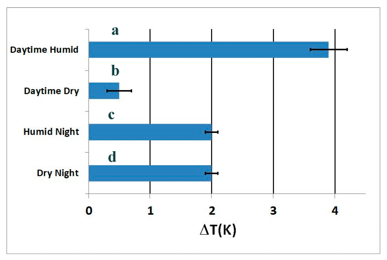
In general, Zhao et al. made a key observation: “Twenty-four of the cities are located in the humid southeast United States, which coincides roughly with the Koppen–Geiger temperate climate zone (see Figure 2a in Ref. [1]). Their daytime annual-mean ∆T is on average 3.9 K and is 3.3 K higher than that of the 15 cities in the dry region (Zhao et al. Figure 2d,e). By comparison, the night-time ∆T differs by 0.1 K between the two groups (Zhao et al. Figure 2f,g).” These data are summarized in Table 1 (also see Figure 1).

Equation (5) can be written for the special case when ${\overline{T}}_{Ru\_Wet}={\overline{T}}_{U\_Dry}^{}$:

$$\Delta {\overline{R}}_{We{t}_U-Dr{y}_U,daytime}\approx {\overline{P}}_{Wet\_U}-{\overline{P}}_{Dry\_U}=\epsilon \sigma f_{\mathrm{X},\mathrm{Y},\mathrm{Z}=30\mathrm{m}}(\Delta q)\left({({\overline{T}}_{U-Dry}+3.3\mathrm{K})}_{}^4-{\overline{T}}_{U-Dry}^4\right)$$

(6)

It is necessary to obtain estimates for this special case when ${\overline{T}}_{Ru\_Wet}={\overline{T}}_{U\_Dry}^{}$, as it allows for simplified results. However, this is a reasonable case to assess since estimates are affected primarily by the temperature difference that averages 3.3 K between wet and dry urban environments in similar cities, and the results are understood to be for this particular case. Here f_{X,Y,Z = 30 m} is a generalized location factor that has been averaged in the Zhao et al. data at a height of Z = 30 m. Then, relative to their findings, f is set at unity. Then, an estimate of the WVF from the UHI temperature difference data can be obtained using Equation (5) for a specific height, f = 1, as detailed in the general WVF model in Equation (14) and in Section 3, giving:

$${\lambda }_{W_U-D_U}\approx \Delta {\overline{R}}_{We{t}_U-Dr{y}_U}(\Delta T_U)/\Delta T_{Wet-Dry,S}$$

(7)

Then, the UHI ∆T water-vapor feedback model (WVFM) simplifies to:

$${\lambda }_{W_U-D_U}\approx \epsilon \sigma \left({({\overline{T}}_{U-Dry}+\Delta T_{Wet})}_{}^4-{\overline{T}}_{U-Dry}^4\right)/\Delta T_{Wet-Dry,S}$$

(8)

Although the actual $\overline{T}$ measurement value may not be known, a range can be considered.

2.3. Temperature Data

Here, a simplified overview of Zhao et al.’s data is presented in Figure 1, primarily to aid the reader and provide support for Zhao et al.’s dataset, which is incorporated into Equation (6). For simplicity, their direct MODIS dataset was selected for comparisons.

Figure 1, bar a, is from Zhao et al.’s Figure 2e, humid climate (MODIS only), and is also similar in values to their Figure 2b. Figure 1, bar b, is from the dry climate daytime results in their Figure 2d. Figure 1, bar c, is from the mild humid nighttime climate results in their Figure 2g. Figure 1, bar d, is from the nighttime dry climate results in their Figure 2f. The ∆T_Wet = 3.3 K value is evident in Figure 1, taken from the Zhao et al. MODIS data, where the average ∆T_Wet ≈ 3.9 K (in Zhao et. al., Figure 2d,e) compared to the daytime dry value of about ∆T_Wet ≈ 0.5 K, and the difference is about 3.4 K, close to the 3.3 K value in their statement (with error bars, 1 s.e. whiskers, shown in the figure). Note that Figure 1 bar c for humid night and bar d for dry night shows no differences. Their measurements were taken at a 30 m height at 1:00 and 13:00 local time on clear days. This is also summarized in Table 1.

3. Results

In Zhao et al.’s data, although no direct measurements of $\overline{T}$ were provided, an initial estimate of the potential radiative difference between dry and humid climates can be provided. For example, using the average temperature of the earth, T_U-Dry = 288 K (15 °C), and the mean for ∆T_Wet = 3.3 K, with a standard error in their convection cooling data of ±0.3 K, yields:

$$\begin{array}{l}\Delta {\overline{R}}_{We{t}_U-Dr{y}_U}=\{\begin{array}{l}\epsilon \sigma {\left({({\overline{T}}_{U-Dry}+3.3\mathrm{K})}_{}^4-{\overline{T}}_{U-Dry}^4\right)}_{Z=30\mathrm{m},Daytime}=11.3\pm 1.04{\mathrm{Wm}}^{-2}\\ \epsilon \sigma {\left({({\overline{T}}_{U-Dry}+0\mathrm{K})}_{}^4-{\overline{T}}_{U-Dry}^4\right)}_{Z=30\mathrm{m},Nighttime}=0\end{array}\\ \end{array}$$

(9)

for ${\overline{T}}_{Ru\_Wet}={\overline{T}}_{U\_Dry}^{}$.

Note that a standard error (s.e.) of ±0.3 for ∆T_Wet yields an s.e. for $\Delta \overline{R}$ of ±1.04 Wm⁻². Here, a value of ε = 0.62 [22,23] is used. This value of ε is comparable to the Liu et al. data measurement (see Equation (13)) and is the average value for the effective emissivity constant for the planetary system, referenced to the top of the atmosphere (i.e., outgoing longwave radiation OLR~εσT⁴_s). Then, it is possible to come up with a rough approximation for the water-vapor feedback, λ~dOLR/dTs (per Equation (8)). ∆T(q)_U-Wet dominated the Zhao et al. daytime observation, yielding the higher observed UHI temperature in the humid environment. This was not observed (Figure 1c,d) in the Zhao et al. [1] nighttime data for humid vs. dry cities, and the model agrees, finding $\Delta \overline{R}=0$ in Equation (9), as required. For the daytime example, at an average UHI temperature of ${\overline{T}}_{U-Dry}=15°\mathrm{C}$ and ∆T_Wet = 3.3 K, the UHI water-vapor feedback ${\lambda }_{W_U-D_U}$ wet-biased estimate from Zhao et al.’s dataset (see Equations (7), (8) and (14)) with $\Delta T_{Wet-Dry,S}=3.3\mathrm{K}$ yields:

$$\begin{array}{c}{\lambda }_{W_U-D_U}|{}_{30\mathrm{m},\mathit{Daytime}}=11.3\mathrm{W}/{\mathrm{m}}^2/3.3\mathrm{K}=3.43\pm 0.32{\mathrm{Wm}}^{-2}{\mathrm{K}}^{-1}\mathrm{for}\\ {\overline{T}}_{Ru\_Wet}={\overline{T}}_{U\_Dry}^{}\end{array}$$

(10)

Using this method, ${\lambda }_{W_U-D_U}$ wet-biased estimates can be provided for a range of 5 °C < ${\overline{T}}_U$ < 30 °C in Equation (9), yielding:

$$3.1\pm 0.32{\mathrm{Wm}}^{-2}{\mathrm{K}}^{-1}<{\lambda }_{W_U-D_U}|{}_{30\mathrm{m},\mathrm{Day}}<4.0\pm 0.32{\mathrm{Wm}}^{-2}{\mathrm{K}}^{-1},for5°\mathrm{C}<{\overline{T}}_{U-Dry}<30\text{°}\mathrm{C}$$

(11)

where ${\overline{T}}_{Ru\_Wet}={\overline{T}}_{U\_Dry}^{}$.

The three-standard-error range is fairly wide, given a sample size of 24 wet cities and their mean and s.e. Therefore, the 99 percent Student’s t confidence range has a reasonably smaller range of approximately $\pm 0.19{\mathrm{Wm}}^{-2}{\mathrm{K}}^{-1}$. That is, if we repeated these measurements, 99 times out of 100 the results should fall within this $\pm 0.19{\mathrm{Wm}}^{-2}{\mathrm{K}}^{-1}$ range.

Note that the Equation (11) result is fairly consistent with the heatwave assessments that humidity amplification is correlated with warming temperature levels That is, we note that the WVF results are greater at 30 °C than 5 °C. For example, Russo et al. (2017) [15] found that the magnitudes and apparent temperature peaks of heatwaves suggest that amplification by humidity increases with increasing warming levels, in agreement with the Equation (11) results.

3.1. Generalized Model to Reproduce Literature Results

Lastly, it is important to show how the UHI ∆T WVF model can be used to make comparisons to literature results to illustrate that the UHI water-vapor feedback model yields reasonable results. Equation (8) can be generalized for this purpose by providing a ∆T WVFM for global (Gl) warming temperature difference data, similar to Equation (8), where:

$$\begin{array}{ll}{\lambda }_{W_U-D_U}& =\Delta {\overline{R}}_{Gl\_Wet-Gl\_Dry}/\Delta {\overline{T}}_{Gl}\approx \left({\overline{P}}_{Gl\_Wet}-{\overline{P}}_{Gl\_Dry}\right)/\Delta {\overline{T}}_{Gl}\\ & =\epsilon \sigma \left({({\overline{T}}_{Gl\_Wet})}_{}^4-{\overline{T}}_{Gl\_Dry}^4\right)/\Delta {\overline{T}}_{Gl}\\ & =\epsilon \sigma \left({({\overline{T}}_{Gl\_Dry}+\Delta {\overline{T}}_{WVF}(\Delta q))}_{}^4-{\overline{T}}_{Gl\_Dry}^4\right)/\Delta {\overline{T}}_{Gl}\end{array}$$

(12)

Here, $\Delta T_{WVF}$ is the estimated global warming average temperature change due to WVF, ${\overline{T}}_{Gl\_Dry}$ is the earth’s average temperature minus the anomaly (i.e., before climate change), and $\Delta T_{Gl}$ is the global warming temperature change anomaly. This can help us gain confidence in the estimates in Equations (10) and (11), for example, if literature values can be reproduced with this similar generalized ∆T WVF model.

To accomplish this, we first need some ∆T data. Appendix A provides an assessment of the Liu et al. (2010) results. Equation (A2) in Appendix A finds that WV was responsible for a temperature increase of ∆T_WVF = 0.298 °C out of global temperature rise at the time of Liu et al.’s [4] assessment of approximately 0.64 K. The global mean temperature in 2010 (see

Table 2. UHI and general water-vapor feedback model results.

UHI Water-Vapor Feedback Model Results From Equation (8)
Authors	Average Year	Period of Study	ε	$\Delta T_{Wet}$(K)	$\Delta T_{}$${}_{Wet-Dry,S}$	${\overline{T}}_{U-Dry}^{}$	λ (Wm−2K−1) UHI ∆T WVFM Equation (8)	λ (Wm−2K−1) Reported
Zhao et al. (2014) [1]	2008	2003–2012	0.62	3.3 K	3.3 K	5 °C	3.1 ± 0.3	NA
Zhao et al. (2014) [1]	2009	2003–2012	0.62	3.3 K	3.3 K	15 °C	3.4 ± 0.3	NA
Zhao et al. (2014) [1]	2010	2003–2012	0.62	3.3 K	3.3 K	30 °C	4.0 ± 0.3	NA
Generalized Water-Vapor Feedback Model Used to Reproduce Literature Results From Equation (12)
Authors	Average Year	Period of Study	ε	∆T Due to WV Feedback	Global Warming (K)	Average Earth Temp.	λ (Wm−2K−1) ∆T WVFM Equation (12)	λ (Wm−2K−1) Reported Average
Liu et al. (2018) [4]	2010	2004–2016	0.62	0.298 *	0.64 *	13.73 °C	1.55	1.55
Gordon et al. (2013) [24]	2006	2003–2008	0.89	0.288 *	0.62 *	13.72 °C	2.39	2.4
Dessler et al. (2008) [21]	2006	2002–2009	0.815	0.288 *	0.62 *	13.72 °C	2.19	2.2

* See Appendix A and Section 3.1.

) if climate change did not occur is estimated to have a value $\overline{T}=13.74°\mathrm{C}=286.89\mathrm{K}$. Then, similar to Equation (9), the results yield:

$$\begin{array}{ll}{\lambda }_{W_U-D_U}& =\epsilon \sigma \left({(286.89\mathrm{K}+0.298\mathrm{K})}_{}^4-{(286.89\mathrm{K})}_{}^4\right)/0.64\mathrm{K}\\ & =1.55{\mathrm{Wm}}^{-2}{\mathrm{K}}^{-1}\end{array}$$

(13)

This result reproduces the water-vapor feedback measurement by Liu et al. (2018). This is discussed in Section 4 (see Table 2). To match their results, a value of ε =0.62 is needed. This is the average value for the effective emissivity constant for the planetary system [22,23]. In addition, this value is used in Equations (10) and (11). The model was also used for Gordon et al. (2013) [24] and Dressler et al.’s (2008) [21] results. However, in their cases, the model finds that a higher ε value is required to match their numbers. Therefore, the Liu et al. assessment appears to be more relevant for comparisons. From this point of view, comparing Equations (10)–(13) (with similar average temperatures of $\overline{T}=13.7°\mathrm{C}$ and $15°\mathrm{C}$, the UHI ∆T water-vapor feedback in wet environments is a little over twice as high compared to Liu et al.’s (2018) [4] results. This assessment helps to provide a measure of credibility to the UHI temperature difference WVFM. It indicates that the WVF value found based on the Zhao et al. (2014) measurements is rigorous and can be compared to global estimates with reasonable confidence.

Table 2 summarizes the water-vapor feedback modeling estimates, including the model’s findings in reproducing literature results based on average temperature differences (see Equations (8) and (12)).

4. Discussion

Global water-vapor feedback is strongly positive, and estimates vary. For example, Dessler et al. (2008) [21] estimated a climate feedback average of λ = 2.04 Wm⁻²K⁻¹ (for the short-term period of 2003–2008), with yearly variation between 0.94 Wm⁻²K⁻¹ and 2.69 Wm⁻²K⁻¹, Gordon et al.(2013) [24] estimated 1.9 Wm⁻²K⁻¹–2.8 Wm⁻²K⁻¹ (for the period of 2002–2009), and Liu et al. (2018) [4] estimated the short-term value of 1.55 Wm⁻²K⁻¹ (for the years 2004–2016).

Dessler et al. (2008) [21] found that, “It is tropical changes in specific humidity (q) that primarily determines the size of the water-vapor feedback, and tropical q is primarily regulated by the tropical surface temperature.” Dessler et al. found that years with milder surface temperature change led to lower water-vapor change and lower water-vapor feedback. For example, a value of 0.94 Wm⁻²K⁻¹ was found in the year 2007, corresponding to a lower tropic surface temperature change. One can make a comparison to the results in Equation (11), where for wet-biased cities, as the average UHI temperature decreases, so does the water-vapor feedback. Moreover, many cities exhibit tropic-like conditions in high humidity environments.

The results of Equation (11) are also consistent with Colman and McAvaney (2009) [25] and Jonko et al. (2013) [26], who also found an increase in water-vapor feedback strength in warmer climates.

Liu et al. (2018) [4] noted that, “the tropics dominate the strength of global mean feedback because long-wavelength water-vapor kernels dominate over the deep tropics…” In this study, wet-biased UHIs, per Zhao et al.’s observations, have a measure of tropical-like climate conditions due to the elevated heat island effect.

Furthermore, the model results indicate that water-vapor feedback is 3.4 Wm⁻²K⁻¹ (Equation (10)), for a temperature rise of 3.3K in wet-biased UHI environments at 15 °C. This does not seem high in comparison to Equation (A2) in Appendix A. Equation (A2) indicates that we can associate a global water-vapor feedback of 1.55 Wm⁻²K⁻¹ (Liu et al., 2013) with a WV feedback temperature increase of $\Delta {\overline{T}}_{WVF}=0.298°\mathrm{C}$ (Table 2). This is an eleven times lower temperature difference value than the UHI temperature change. By comparison, one could argue that the preliminary findings of these UHI water-vapor feedback estimates from the model are not high, considering its associated environmental temperature change with a large ∆T of 3.3 K. In addition, the model was able to reproduce the literature findings of Liu et al., Gordon et al., and Dessler et al. (see Table 2) using temperature difference data for their measurement periods. Therefore, these model results appear credible. We indicated that the Liu et al. (2018) results were the most comparable where the ε value matched the average value for the effective emissivity constant for the planetary system [22,23] used in the UHI ∆T WVFM assessment. Therefore, the ∆T WVF model results appear to provide rigorous values based on the data.

Since the UHI ∆T WVFM results used a limited dataset of 39 cities, with results at 30m, the findings should be considered preliminary. However, the results certainly show concerns for a strong local UHI water-vapor feedback issue for cities in humid environments, suggesting that actual feedback measurements should be performed to verify the magnitude. Furthermore, there is concern that water-vapor is strongly interactive with cities, as shown by the numerous heatwave studies (see Section 1) in humid areas. However, as was pointed out, direct measurements could be very challenging due to temperature lapse-rate effects, with possible temperature inversions occurring amongst tall UHI buildings. Due to this anticipated difficulty in making measurements and the unlikely challenge of repeating a similar study comparable to the magnitude of the Zhao et al. work, providing a preliminary water-vapor feedback assessment is needed and important.

The common use of the feedback equation is to partition it into two terms. However, it does not need to be partitioned, and modeling shows it can be extended for use with the UHI ∆T observations to provide a preliminary comparative estimate where:

$$\begin{array}{c}{\lambda }_q={\left({\displaystyle \sum _{x,y,z}\frac{\partial R_{OLR}}{\partial q(x,y,z)}\frac{\Delta q(x,y,z)}{\Delta T_S}}\right)}_{General}\\ \to {\left({\displaystyle \sum _{UHIs}\frac{\Delta {\overline{R}}_{Wet-Dry,OLR-UHI}(\Delta T)f_{XYZ}(\Delta q)}{\Delta T_{Wet-Dry,S}}}\right)}_{ExtendedtoUHIs}\end{array}$$

(14)

Extending the equation’s applicability to Zhao et al.’s data with the UHI ∆T WVFM (Equations (7) and (8)) is reasonable since it was a very unique and carefully conducted study that had strong water-vapor UHI observation.

Measurements such as those by Dessler et al., Gordon et al., and Liu et al. did not focus on estimating the feedback attributed to humid areas at low portions of the troposphere due to UHI growth. This leaves a large gap, as 55% of the population now lives in, and this number is expected to increase to near 70% by 2050 [10]. For many of these cities, humidity often plays a role in amplifying temperature problems.

Note that because Equation (11) indicates a lower temperature change produces less feedback, albedo management is likely a key solution. Although there are many ways to cool cities by design, for existing cities albedo management is likely the most practical approach. This would also help mitigate exacerbated UHI heatwaves. Albedo management was also suggested by Zhao et al.

In this case, it is desirable to restore UHIs to their original estimated albedo value before their existence. In a prior study [27,28], it was estimated that an albedo value of 0.2 (pre-UHI era) removes the urbanization forcing effect. Note that an average UHI albedo value from the author’s prior study [27,28] was 0.12 due to Sugawara et al. (2014) [29].

The solar geoengineering of UHIs has been studied, and increasing the UHI albedo by about 0.1 is feasible. In a paper by Akbari et al. (2012) [30], it was estimated that, “white rooftops and light-colored pavements, can increase the albedo of urban areas by about 0.1 and could potentially offset some of the anticipated temperature increase caused by global warming.”

5. Conclusions

In this paper, a water-vapor feedback model for UHI daytime humid environments was developed and used specifically to convert Zhao et al.’s (2014) ∆T dataset to provide water-vapor feedback estimates. The Zhao et al. study provided a unique observed UHI ∆T dataset with daytime data on 24 wet-biased cities compared to 15 dry UHI cities. The developed targeted model was used to convert their ∆T observations to UHI local water-vapor feedback values. The model provided preliminary daytime water-vapor feedback wet-biased estimates of 3.1 Wm⁻²K⁻¹, 3.4 Wm⁻²K⁻¹ 4 Wm⁻²K⁻¹ for UHI average temperatures of 5 °C, 15 °C, and 30 °C, respectively (see Table 2). The model also provided negligible nighttime WVFM estimates, as observed. Furthermore, the model showed that the water-vapor feedback increases with the average UHI temperature. The results were for Zhao et al.’s measurements taken at 30 m and averaged over the thirty-nine cities. Thus, the measurement heights and city sample size provide limited data for analysis. Therefore, we caution that the results are a preliminary assessment.

The UHI ∆T WVFM was generalized to be used for global average temperature difference data. The generalized temperature difference WVFM reproduced the water-vapor feedback measurements by Liu et al. (2018), Gordon et al. (2013), and Dressler (2008). The results indicated that the Liu et al. assessment appears to be more relevant for comparisons since the results matched the average value for the effective emissivity constant, $f\approx {\epsilon }_{eff}$, for the planetary system that was also used in the UHI work. From this point of view, UHI water-vapor feedback in wet environments was a little over twice as high compared to Liu et al.’s (2018) results. Extending the UHI temperature difference WVF model to global assessments provided a measure of confidence to the UHI temperature difference WVFM and indicated that the WVF value based on the Zhao et al. (2014) measurements was reasonably validated through modeling comparisons.

Overall, these rigorous preliminary modeling estimates show strong concerns for high water-vapor feedback in UHIs with humid environments. Follow-up UHI water-vapor feedback verification measurements are suggested.

Albedo management for humid hotter cities should be a priority both for local health reasons, to reduce water-vapor feedback and to reduce UHI heatwave exacerbation effects, and to reduce UHI global warming contributions [31]. Recent trends suggest that urbanization is contributing more to global warming than previously assessed (contributing as much as 13%; [28,31,32]. Considering that WVF in UHIs in humid environments amplifies heat and can exacerbate heatwave severity, frequency, and duration, cities in humid environments are likely larger contributors to such warming trends compared to cities in dry regions. Unfortunately, both greenhouse gases and UHIs are growing roughly with population size [27]. In China, a temporal study by Yang et al. (2018) [33] of 302 cities found higher UHI growth rates than the population growth rate by about a factor of 4.5% per year from 2003 to 2016. Both GHGs and UHIs are affecting climate change [28,31]. However, a coordinated worldwide effort to focus on the UHI problem is lacking, as there are no mitigation details in the Paris Accord, despite the concern of many UHI authors [27,31,33,34,35,36,37,38,39]. It was pointed out that there are many reasons for the albedo management of UHIs in both dry and wet environments. This study provides strong support for including UHI albedo management in the Paris Accord goals.

References

- Zhao, L.; Lee, X.; Smith, R.; Oleson, K. Strong, contributions of local background climate to urban heat islands. Nature 2014, 511, 216–219. [Google Scholar] [CrossRef] [PubMed]
- Watts, N.; Amann, M.; Arnell, N.; Ayeb-Karlsson, S.; Beagley, J.; Belesova, K.; Boykoff, M.; Byass, P.; Cai, W.; Campbell-Lendrum, D.; et al. The 2020 report of The Lancet Countdown on health and climate change: Responding to converging crises. Lancet 2021, 397, 129–170. [Google Scholar] [CrossRef]
- Tuholske, C.; Caylor, K.; Funk, C.; Verdin, A.; Sweeney, S.; Grace, K.; Peterson, P.; Evans, T. Global urban population exposure to extreme heat. Proc. Natl. Acad. Sci. USA 2021, 118, e2024792118. [Google Scholar] [CrossRef]
- Liu, R.; Su, H.; Liou, K.; Jiang, J.; Gu, Y.; Liu, S.; Shiu, C. An Assessment of Tropospheric Water Vapor Feedback Using Radiative Kernels. JGR Atmos. 2018, 123, 1499–1509. [Google Scholar] [CrossRef]
- Kovats, S.; Hajat, S. Heat Stress and Public Health: A Critical Review. Annu. Rev. Public Health 2008, 29, 41–55. [Google Scholar] [CrossRef]
- Changnon, S.; Kunkel, K.; Reinke, B. Impacts and responses to the 1995 heat wave: A call to action. Bull. Am. Meteorol. Soc. 1996, 77, 1497–1506. [Google Scholar] [CrossRef]
- Buechley, R.; Van Bruggen, J.; Trippi, L. Heat island equals death island? Environ. Res. 1972, 5, 85–92. [Google Scholar] [CrossRef]
- Burke, M.; Hsiang, S.; Miguel, E. Global non-linear effect of temperature on economic production. Nature 2015, 527, 235–239. [Google Scholar] [CrossRef]
- Day, E.; Fankhauser, S.; Kingsmill, N.; Costa, H.; Mavrogianni, A. Upholding labor productivity under climate change: An assessment of adaptation options. Clim. Policy 2019, 19, 367–385. [Google Scholar] [CrossRef]
- Worldbank, Urban Development. 2020. Available online: https://www.worldbank.org/en/topic/urbandevelopment/overview#1 (accessed on 2 January 2022).
- Wang, P.; Yang, Y.; Tang, J.; Leung, L.; Liao, H. Intensified Humid Heat Events Under Global Warming. Geophys. Res. Lett. 2021, 48, e2020GL091462. [Google Scholar] [CrossRef]
- Li, D.; Bou-Zeid, E. Synergistic interactions between urban Heat Islands and heat waves: The impact in cities is larger than the sum of its parts. J. Appl. Meteorol. Climatol. 2013, 52, 2051–2064. [Google Scholar] [CrossRef] [Green Version]
- Liao, W.; Liu, X.; Li, D.; Luo, M.; Wang, D.; Wang, S.; Baldwin, J.; Lin, L.; Li, X.; Feng, K.; et al. Stronger Contributions of Urbanization to Heat Wave Trends in Wet Climates. Geophys. Res. Lett. 2018, 45, 11310–11317. [Google Scholar] [CrossRef] [Green Version]
- Li, C.; Sun, Y.; Zwiers, F.; Wang, D.; Zhang, X.; Chen, G.; Wu, H. Rapid Warming in Summer Wet Bulb Globe Temperature in China with Human-Induced Climate Change. J. Clim. 2020, 33, 5697–5711. [Google Scholar] [CrossRef] [Green Version]
- Russo, S.; Sillmann, J.; Sterl, A. Humid heat waves at different warming levels. Sci. Rep. 2017, 7, 7477. [Google Scholar] [CrossRef] [Green Version]
- Kong, D.; Gu, X.; Li, J.; Ren, G.; Liu, J. Contributions of Global Warming and Urbanization to the Intensification of Human-Perceived Heatwaves Over China. JPG Atmos. 2020, 125, e2019JD032175. [Google Scholar] [CrossRef]
- Zou, Z.; Yan, C.; Yu, L.; Jiang, X.; Ding, J.; Qin, L.; Wang, B.; Qiu, G. Impacts of land use/ land cover types on interactions between urban heat island effects and heat waves. Build. Environ. 2021, 204, 108138. [Google Scholar] [CrossRef]
- Yang, X.; Ruby Leung, L.; Zhao, N.; Zhao, C.; Qian, Y.; Hu, K.; Liu, X.; Chen, B. Contribution of urbanization to the increase of extreme heat events in an urban agglomeration in east China. Geophys. Res. Lett. 2017, 44, 6940–6950. [Google Scholar] [CrossRef]
- Bornstein, R. Observations of the Urban Heat Island Effect in New York City. J. Appl. Meteorol. (1962–1982) 1968, 7, 575–582. [Google Scholar] [CrossRef]
- Fast, J.; Torcolini, J.; Redman, R. Pseudovertical Temperature Profiles and the Urban Heat Island Measured by a Temperature Datalogger Network in Phoenix, Arizona. J Appl. Meteorol. 2005, 44, 3–13. [Google Scholar] [CrossRef]
- Dessler, A.; Zhang, Z.; Yang, P. Water-vapor climate feedback inferred from climate fluctuations, 2003–2008. Geophys. Res. Lett. 2008, 35, L20704. [Google Scholar] [CrossRef]
- Kimoto, K. On the Confusion of Planck Feedback Parameters. Energy Environ. 2009, 20, 1057–1066. [Google Scholar] [CrossRef]
- Feinberg, A. A Re-radiation Model for the Earth’s Energy Budget and the Albedo Advantage in Global Warming Mitigation. Dyn. Atmos. Ocean. 2022, 97, 101267. [Google Scholar] [CrossRef]
- Gordon, N.D.; Jonko, A.K.; Forster, P.M.; Shell, K.M. An observationally based constraint on the water-vapor feedback. JGR Atmos. 2013, 118, 12435–12443. [Google Scholar] [CrossRef] [Green Version]
- Colman, R.A.; McAvaney, B. Climate feedbacks under a very broad range of forcing. Geophys. Res. Lett. 2009, 36, L01702. [Google Scholar] [CrossRef]
- Jonko, A.K.; Shell, K.; Sanderson, B.; Danabasoglu, G. Climate feedbacks in CCSM3 under changing CO2 forcing. Part II: Variation of climate feedbacks and sensitivity with forcing. J. Clim. 2013, 26, 2784–2795. [Google Scholar] [CrossRef]
- Feinberg, A. Urban heat island amplification estimates on global warming using an albedo model. SN Appl. Sci. 2020, 2, 2178. [Google Scholar] [CrossRef]
- Feinberg, A. Solar Geoengineering Modeling and Applications for Mitigating Global Warming: Assessing Key Parameters and the Urban Heat Island Influence. Front. Clim. 2022, 4, 870071. [Google Scholar] [CrossRef]
- Sugawara, H.; Takamura, T. Surface Albedo in Cities (0.12) Case Study in Sapporo and Tokyo, Japan. Bound.-Layer Meteorol. 2014, 153, 539–553. [Google Scholar] [CrossRef]
- Akbari, H.; Matthews, D.; Seto, D. The long-term effect of increasing the albedo of urban areas. Environ. Res. Lett. 2012, 7, 024004. [Google Scholar] [CrossRef]
- Zhang, P.; Ren, G.; Qin, Y.; Zhai, Y.; Zhai, T.; Tysa, S.K.; Xue, X.; Yang, G.; Sun, X. Urbanization Effects on Estimates of Global Trends in Mean and Extreme Air Temperature. J. Clim. 2021, 34, 1923–1945. Available online: https://journals.ametsoc.org/view/journals/clim/34/5/JCLI-D-20-0389.1.xml (accessed on 2 January 2022). [CrossRef]
- Feinberg, A. Anthropogenic Heat Release with Secondary Effects Significantly Impacts Global Warming: UHI Mitigating Solar Geoengineering Requirements, Preprint at ResearchGate. 2022. Available online: https://www.researchgate.net/publication/364365387_Anthropogenic_Heat_Release_with_Secondary_Effects_Significantly_Impacts_Global_Warming_UHI_Mitigating_Solar_Geoengineering_Requirements?_sg=FtDUTuT0p-an5PxRA6iQlBs1oucid0kIA1oNo0o4D3ZeTgN4epH4mZM8n6KzY6hTLKA5qaILaI-Ihf0 (accessed on 20 October 2022).
- Yang, Q.; Huang, X.; Tang, Q. The footprint of urban heat island effect in 302 Chinese cities: Temporal trends and associated factors. Sci. Total. Environ. 2019, 655, 652–662. [Google Scholar] [CrossRef] [PubMed]
- Feddema, J.J.; Oleson, K.W.; Bonan, G.B.; Mearns, L.O.; Buja, L.E.; Meehl, G.A.; Washington, W.M. The importance of land-cover change in simulating future climates. Science 2005, 310, 1674–1678. [Google Scholar] [CrossRef] [Green Version]
- De Laat, A.T.J.; Maurellis, A.N. Evidence for the influence of anthropogenic surface processes on lower tropospheric and surface temperature trends. Int. J. Climatol. 2006, 26, 897–913. [Google Scholar] [CrossRef]
- Ren, G.; Chu, Z.; Chen, Z.; Ren, Y. Implications of temporal change in urban heat island intensity observed at Beijing and Wuhan stations. Geophys. Res. Lett. 2007, 34, L05711. [Google Scholar] [CrossRef]
- Ren, G.Y.; Chu, Z.Y.; Zhou, J.X. Urbanization effects on observed surface air temperature in North China. J. Clim. 2008, 21, 1333–1348. [Google Scholar] [CrossRef] [Green Version]
- Huang, Q.; Lu, Y. Effect of Urban Heat Island on Climate Warming in the Yangtze River Delta Urban Agglomeration in China. Int. J. Environ. Res. Public Health 2015, 12, 8773–8789. [Google Scholar] [CrossRef] [Green Version]
- Sun, Y.; Zhang, X.; Ren, G.; Zwiers, F.; Hu, T. Contribution of urbanization to warming in China. Nat. Clim. Chang. 2016, 6, 706–709. [Google Scholar] [CrossRef]
- NASA Global Climate Change Website. 2022. Available online: https://climate.nasa.gov/vital-signs/global-temperature/ (accessed on 2 January 2022).
- Manabe, S.; Wetherald, R.T. Thermal equilibrium of atmosphere with a given distribution of relative humidity. J. Atmos. Sci. 1967, 24, 241–259. [Google Scholar] [CrossRef]
- Randall, D.; Wood, R.; Sandrine, B.; Colman, R.; Fichefet, T.; Fyre, J.; Kattsov, V.; Pitman, A.; Shukla, J.; Srinivasan, J.; et al. Climate Models and Their Evaluation, in Climate Change 2007: The Physical Science Basis. Contributions of Working Group I to the Fourth Assessment Report of the Intergovernmental Panel on Climate Change; Cambridge University Press: Cambridge, UK, 2007. [Google Scholar]
Figure 1.
Key estimates were taken from Zhao et al.’s MODIS ∆T data (see theirtable). The assessed values are (a) the daytime value of humid cities, (b) the daytime value in dry cities, (c,d) the nighttime value of humid cities, and (d) the nighttime value of dry cities. Error bars: 1 s.e.