
To What Extent Have Nature-Based Solutions Mitigated Flood Loss at a Regional Scale in the Philadelphia Metropolitan Area?
Department of Geography and Urban Studies, Temple University, Philadelphia, PA 19122, USA
Urban Sci. 2023, 7(4), 122; https://doi.org/10.3390/urbansci7040122
Submission received: 27 August 2023
/
Revised: 10 November 2023
/
Accepted: 21 November 2023
/
Published: 4 December 2023
(This article belongs to the Special Issue Water Resources Planning and Management in Cities)
Abstract
:Globally, floods are becoming more severe, lasting longer, and occurring more frequently because of changes in climate, rapid urbanization, and changing human demographics. Although traditional structural flood mitigation infrastructures (e.g., drainage systems, levees) are effective in urban areas, their functionalities in the face of extreme rainfall events and increased development largely depend on the capacity and location of such systems, making complementary solutions such as nature-based solutions (NBS) important. The concept of NBS within the context of flood mitigation has gained traction in the last decade; however, the success of NBS depends on their effectiveness and distribution over urban regions. This article seeks to examine the potential of NBS as a flood loss mitigation tool in one of the fastest-growing and flood-prone counties of Pennsylvania, Montgomery County, using Generalized Linear Model (GLR) and Geographically Weighted Regression (GWR) techniques. The analysis integrates the National Risk Index dataset for river flooding, a 100-year flood zone layer from National Flood Hazard Layer (NFHL) provided by FEMA, with land use and impervious surface percent data derived from National Land Cover Database (NLCD) for 2019 and socioeconomic data at the U.S. census tract level from the 2019 U.S. Census. This study’s findings partially contradict previous research by revealing an unexpected relationship between NBS quantity in floodplains and expected annual loss. Findings also suggest that small size and disconnected patches of NBS in floodplains in some dense urban areas effectively reduce total losses from flood events.
1. Introduction
Urban and regional environments have experienced significant transformations due to rapid urbanization, leading to a myriad of challenges. This is especially pronounced in densely populated urban areas where the proliferation of grey infrastructure, such as highways, parking lots, and towering buildings, has increased the risk of flooding. Various studies, including those by [1,2,3,4] indicate that climate change and alterations in land use/land cover (LULC), which involve the substitution of vegetated regions with impervious surfaces like roads, rooftops, and parking lots, exacerbate the damaging effects of floods.
Additionally, floods are becoming more severe, lasting longer, and occurring more frequently because of changes in climate, rapid urbanization, and changing human demographics globally and throughout the United States (US) [5,6]. Direct flood damages in the United States have cost a total of $99 billion and more than 1000 deaths over the last 10 years, with an upward trend in flood losses over time [7]. The findings of a recent study show a 26.4% increase in US floods by 2050 under intermediate climate change scenarios of RCP4.5 [8]. In 2021, Hurricane Ida caused an estimated $16 to 24 billion in flooding damage in the Northeastern United States, making it the most expensive storm to impact the region since Hurricane Sandy in 2012, with an estimated $44 billion in insured loss [9]. In addition, about 83% of the population lives in urban areas in the United States today, with 89% (400 million) of the national population projected to live in cities by 2050 [10]. A once-in-100-year flood threatens 41 million people in the United States alone (Wing et al., 2018). According to projections, urban land cover will nearly double over croplands and forests by 2050 in the U.S. [11,12], causing the degradation of the local and national ecosystem, exacerbating climate change, human health, and global warming [3,4].
Over the two last decades, several adaptation and mitigation policies (e.g., channels, pipelines, and storage tanks) have been suggested to reduce the risk associated with urban flooding in urban and regional areas [13]. However, the use and upkeep of these traditional approaches have proven to be expensive and insufficient to address the problems posed by increasingly frequent extreme precipitation events associated with climate change and the ensuing floods in metropolitan areas [14]. Nature-based solutions (NBS) (e.g., urban parks, green roofs, floodplains, etc.) are examples of effective adaptation to increased flood risk that can mitigate the negative impacts of climate change and population growth in the river or coastal cities. These measures help restore the natural hydrology of a region, which has been altered by urbanization. Due to beneficial outcomes that enable a more effective reduction of flood impact in urban areas, NBS has become an emerging subject as a flood risk management technique [15].
However, the success of these adaptation strategies depends on their structure, including composition (the quantity and variety of NBS kinds) and configuration (the quality and spatial aspect of NBS types) to reduce flood risk in different regions [16]. Understanding to what extent NBS size within the study area and its spatial characteristics such as shape, connectivity or contiguity could mitigate the risk of flooding would help to facilitate the availability and to increase efficiency of NBS in flooding hazards and its impact [17]. County-level analyses are critical, as they provide a nuanced perspective that considers the unique characteristics and interconnectedness of urban and rural areas within a specific geographic region. Floodplain planning, typically executed at various levels, often falls short of providing detailed insights at the county scale. The intricate dynamics of land use, topography, and existing infrastructure within a county play a pivotal role in influencing the effectiveness of NBS in mitigating flood-related damages. Yet, despite continuous attempts to emphasize the positive influence of NBS in mitigating flood damage, there is a lack of county-scale assessments of the impact of NBS structure for reducing cumulative damages from flooding. A comprehensive county-level analysis offers a more granular understanding of the potential impact of NBS structures on flood-related losses. In the practical realm of NBS planning, it becomes essential to account for the size and shape of the area being considered [18]. This is especially significant in rapidly urbanizing regions where a significant portion of the urban landscape is already occupied by built environments and grey infrastructure [19]. Yet, the results of previous studies at different scales, specifically regarding the configuration of NBS are inconsistent, limiting a comprehensive understanding of the role of these factors in flood reduction [17]. Hence, it becomes crucial to carefully evaluate and optimize the shape and configuration of NBS to fully leverage its potential benefits and enhance its effectiveness in addressing flooding.
To support the above concerns regarding the growing risk of flooding and the effectiveness of NBS structure to mitigate this risk, this paper examines the potential of NBS as a flood loss mitigation tool in one of the fastest-growing counties of Pennsylvania. By focusing on Montgomery County, the research endeavors to enrich our understanding of NBS contributions to flood mitigation at a scale that is often overlooked but holds immense significance for tailored and effective planning and decision-making. This research will address the following question: to what extent have NBS structure in floodplains mitigated flood loss at Montgomery County in the Philadelphia Metropolitan Area? Montgomery County has a long history of flooding over previous decades, including 134 events costing $10 million USD in damages from 1996 to 2019. This study draws on Expected Annual Loss Score (EALS) data associated with flooding from the National Risk Index (NRI) provided by the Federal Emergency Management Agency (FEMA), which has data on total annual loss of buildings, agriculture, and population from flooding from 1996 to 2019. The land cover 2019 map from National Land Cover Database (NLCD) of U.S. Geological Survey was used to realize vegetated NBS (e.g., mangroves, green spaces). This study employs three different spatial statistics methods, including spatial autocorrelation (Global Moran’s I), Generalized Linear Model (GLR), a county regression, and a local regression technique, Geographically Weighted Regression (GWR), to assess non-stationarity in the relationship between NBS composition and configuration and EALS across Montgomery County.
2. NBS and Flood Loss
Conventional structural flood mitigation infrastructure, such as dams and drainage systems, is effective in urban areas, but increasingly inadequate against extreme rainfall events and urban development [20]. For example, in 2018, the abrupt breach of a newly constructed saddle dam at the Xe Nammoy hydroelectric-power reservoir in the Mekong basin, southern Laos, led to catastrophic flooding, resulting in fatalities and the displacement of thousands [21]. Grey infrastructure is expensive, energy-intensive, and lacks the diverse benefits of natural infrastructure-based solutions [20]. Recognizing these limitations, stakeholders, policymakers, and planners are turning to complementary solutions like natural infrastructure and NBS due to their environmental and economic sustainability [17,22]. The International Union for Conservation of Nature (IUCN) defines NBS as “actions that protect, sustainably manage, and restore ecosystems to address societal challenges, providing simultaneous benefits to human well-being and biodiversity” [23]. Recent literature highlights the efficacy of various NBS types, including urban parks, green infrastructure, and water management practices, in enhancing resilience to climate change effects [24]. These solutions facilitate water infiltration, reducing surface runoff during rainfall, while also offering additional advantages like improved air quality, temperature regulation, and enhanced urban aesthetics [25,26,27].
Research on NBS flood mitigation potential is expanding, analyzing how vegetated green infrastructure reduces flood damage and improves resilience [28]. Studies often consider property loss from flooding based on insured claims, demonstrating the significant impact of urban blue-green infrastructure scenarios on reducing property damage [25,29,30]. Yet, few studies have investigated the impact of NBS coverage on property and population loss from flooding in Indian states [31]. While some investigations focus on preserving the size of NBS, studies lack a comprehensive examination of the overall damage from flooding and the influence of NBS configuration on flood loss.
Landscape ecology serves as a valuable framework for understanding the spatial dynamics at the NBS-flood interface across diverse landscapes [32,33]. Research delves into the structure of NBS, examining their impact on flood risk, with a particular focus on runoff mitigation [18,34,35,36]. For example, Bai et al. (2018) and Kim and Park (2016) found that larger urban green spaces (UGS) with diverse and irregular shapes can effectively mitigate stormwater runoff. Other studies conducted in Inner Mongolia (China) and the city of Ghent (Belgium) indicated that the shape of UGS alone may not have a significant influence on flood intensity or the reduction of runoff [37,38]. However, more evidence is needed on the influence of NBS complexity, connectivity, and composition on flooding at the regional scale.
Despite efforts to highlight NBS benefits, additional research is necessary to understand their role in reducing overall property, agriculture, and population losses resulting from flooding. Previous studies focused on insurance claims in coastal areas, neglecting broader implications such as agricultural and population damages. This research aims to address these gaps by examining the potential impact of NBS size and two configurational metrics of shape and connectivity on total property, agriculture, and population loss, utilizing the National Risk Index dataset. The study, conducted in Montgomery County, offers a holistic understanding of NBS impacts on flood-related losses, valuable for flood practitioners, policymakers, and urban planners seeking to enhance their understanding of NBS contributions to mitigating flood damages.
3. Methods
3.1. Study Area
This study focuses on Montgomery County, which is situated in the Philadelphia Metropolitan Area in southeast Pennsylvania (Figure 1). Geographically, Montgomery County exhibits a diverse landscape, ranging from farmland and open countryside in the northern region to densely populated suburban subdivisions in the south and central areas. With a land area of approximately 1250 km2, the county comprises 211 census tracts and is susceptible to flooding from the Schuylkill and Delaware Rivers. Montgomery County is home to over 850,000 residents, and its population continues to grow [39]. The study area experiences a humid subtropical climate, with temperatures ranging from −10.6 °C to 42.2 °C. On average, there are 88 days per year when the minimum daily temperature drops below freezing (0 °C), while there are only 10 days per year when the maximum daily temperature falls below freezing [40].
The area has a long history of flooding [41]. Notably, in September 2021, severe flooding resulting from Hurricane Ida affected a significant portion of Montgomery County along the Schuylkill River. Additionally, Norristown and Conshohocken, cities within the county and with a high percentage of imperviousness (~65%), experienced substantial rainfall, and flooding during Hurricane Irene in August 2011 and Hurricane Ida in 2021, categorizing them as two of the most flood-prone cities in the area [42]. Recent years have witnessed an increase in precipitation intensity attributed to climate change [43]. Moreover, the substantial growth in public and commercial services as well as population rate, which form the primary economic activities in the area, has led to a rapid rise in impervious surfaces, amplifying the risk of flash flooding [40]. The selection of this study area was driven by four main factors: (1) a moderate-to-high risk of flooding over the next 30 years, as projected by Flood Factor and the National Flood Hazard Layer (NFHL) published by FEMA; (2) a relatively high population growth rate (1% between 2010–2020) based on the US Census Bureau 2020; and (3) diverse types of NBS (Figure 1).
3.2. Data
The Expected Annual Loss (EAL) data for flooding in the study area was obtained from the National Risk Index (NRI) dataset, which is provided by the Federal Emergency Management Agency (FEMA) in collaboration with various stakeholders and partners, including academia, local, state, and federal government agencies [44]. The NRI dataset is an online tool designed to identify and illustrate the communities in the United States that are most vulnerable to 18 different natural hazards [45]. In the context of this study, the EAL represents the average economic loss in dollars resulting from flooding each year per census tract. To calculate the Expected Annual Loss Score (EALS) for each consequence type (buildings, population, and agriculture) within each census tract, the NRI dataset quantifies the values of buildings and agriculture in dollars. However, the measurement of population focuses on fatalities and injuries. To establish a standardized unit of measurement, the EAL associated with the population was converted into a population equivalence using a value of statistical life (VSL) methodology [44]. According to this approach, each fatality or every ten injuries is considered equivalent to an economic loss of $11.6 million. To calculate the EALS for river flooding type, the EAL values for the three consequence types (building, population equivalence, and agriculture) are combined. This summation represents the total Expected Annual Loss for flooding within the census tracts of Montgomery County. These values are then compared and ranked across the flooded communities. The Expected Annual Loss score for each census tract is determined based on its national ranking (Figure 2a).
The primary data sources for the explanatory variables are the US census tract-level data for 2019, the land cover 2019 map which was obtained from U.S. Geological Survey’s National Land Cover Database (NLCD), Impervious surface (%) which was taken from NLCD 2019 Percent Developed Imperviousness (CONUS), and American Community Survey (ACS) estimates. NLCD provides 30 m spatial resolution land cover maps for the whole United States and is used to identify vegetated NBS (e.g., mangroves, green spaces). A total of following eight classifications were identified for NBS: open space (21), deciduous forest (41), evergreen forest (42), mixed forest (43), shrub/scrub (52), grassland/herbaceous (71), Pasture/Hay (81), and woody wetlands (90) based on previous studies [16,46,47] (Figure 2).
An additional factor contributing to flooding in the study area is the presence of development within designated flood zones. The Federal Emergency Management Agency (FEMA) has defined a specific geographic area as the flood zone based on the probability of flooding during certain storm return periods. The National Flood Hazard Layer (NFHL), provided by FEMA, includes a 100-year flood zone layer, which is also referred to as the base flood or the one-percent annual chance flood. To examine the relationship between NBS and EALS, population density was considered as a control variable since it directly affects housing and economic activity in the area. The population density data for 2019 was obtained from the US Census Bureau. Population density was measured as the number of residents per acre of the county area. The analysis in this study was conducted using data from 177 populated census tracts within Montgomery County. It is important to note that out of the total 211 census tracts in the county, 23 were excluded from the study as they did not have any flood zones.
Drawing upon the findings of previous studies [17,25,46,48,49], two potential indicators of NBS configuration, namely the shape index (SI) and contiguity index (CONTIG), were computed, specifically tailored to assess flooding at the census tract level. This analysis was conducted using FRAGSTATS version 4.2. SI provides a simple measure of the perimeter and area of a patch and represents the complexity of landscape patch shapes. CONTIG measures the mean number and position of contiguous NBS cells and indicates the spatial connectedness [50]. Higher values of SI and CONTIG represent more complex and contiguous patterns of NBS. It should be emphasized that the high value of isolation alone denotes a NBS condition that is impaired.
Table 1 provides the definition and basic statistics of each index used in the analysis.
3.3. Data Analysis
This study utilized both global and local regression techniques to investigate the spatially varying relationship between NBS area and flood building loss conditions across at two scales: county-wide and local. On the county-wide scale, Generalized Linear Regression (GLR) was employed as a benchmark model, allowing for a comparison with the local models. On the local scale, Geographically Weighted Regression (GWR) was employed to identify unique and spatially explicit relationships within each census tract.
In this study, GLR model was chosen as an appropriate approach for modeling the response variable (EALS), taking into consideration the low spatial dependency. The GLR model allows for the establishment of a linear relationship between predictors and the response, even when the relationship is not inherently linear. The utilization of a link function facilitates this connection between the response variable and the linear model [51]. Collinearity was detected by the variance inflation factor (VIF). To test normal distribution, heteroscedasticity, and spatial autocorrelation, three tests of Jarque-Bera statistics, Breusch-Pagan, and Global Moran’s I were used, respectively, based on previous research [52,53,54].
Unlike traditional linear regression models such as Ordinary Least Squares (OLS), the GLR does not assume a normal distribution of the response variable’s error terms. This divergence from normality is particularly relevant in the context of spatial analysis, where spatial non-stationarity can occur. Linear regression models with constant coefficients, such as OLS, do not account for spatial non-stationarity and may result in deviations from the expected outcomes [55]. GLR is represented as follows:
where f is a function of the mean response “link function”; Yi is the dependent variable EALS at census tract i, βj is regression coefficient, xjp stand for independent variables (IA, PD, NBSF, SI, and CONTIG); and εi is the error.
To address the issue of spatial non-stationarity and capture the spatially varying relationship between the predictors (e.g., NBS variables) and the response variable (EALS), the study employed Geographically Weighted Regression (GWR). GWR offers an alternative to traditional regression analysis by allowing coefficients to vary with geographic position. By decomposing the global relationship into specific geographical units, GWR provides insights into the local dynamics of the relationship and captures spatially explicit patterns [56]. The application of GWR in this study aims to consider the variable relationship between NBS, IA, PD, SI, CONTIG and the EALS variable from a local perspective. This localized analysis enhances our understanding of the specific interactions and impacts of these variables within different geographic locations [57]. It is calculated as follows:
where yi is EALS at census tract i, β0 (ui, vi) represents the intercept at position i; βk (ui, vi) is the coefficient of the kth independent variable estimated for each census tract i at location (ui, vi); and εi is a random error. The integrated GLR and GWR capabilities in the ArcGIS Pro program were used to develop models for social and greenness conditions. For GLR and GWR models, EALS per census tract was regressed against the four variables: NBS size, vegetated NBS size in floodplains, impervious surface percentage, and population density.
The models in this study were compared using two evaluation metrics: the corrected Akaike Information Criterion (AICc) and the adjusted R2. AICc serves as an indicator to assess model performance and to compare the adequacy of GLR and GWR models, as discussed by [58]. In the context of these models, when the AICc difference exceeds 3, a lower AICc value and a higher R-squared value suggest a superior goodness of fit [56]. The adjusted R2 measures the proportion of variance in the response variable explained by the predictors, accounting for the number of predictors and sample size.
4. Results
4.1. Spatial Pattern of NBS
There is higher coverage of NBS in rural and suburban areas, while urban areas exhibit lower NBS presence. The eastern part of the county has higher population density and a greater amount of impervious surface compared to the western part of the county. There are also more census tracts with relatively high and high EALS in East Montgomery, likely due to rapid urbanization and their proximity to the Schuylkill River and Wissahickon Greek. The presence of extensive impervious surfaces in the East County signifies significant development and urban expansion. However, there is a balanced distribution of NBS coverage between the two parts, with denser vegetated NBS in the western region. West Montgomery features a substantial area occupied by golf courses, the Green Lane Reservoir, preserves, Green Lane Park, and primarily low-to-medium-density development. This area boasts a larger quantity of vegetated NBS situated in floodplains, characterized by green corridors and linear parks. Furthermore, the shape index map exhibits a predominant circular pattern, where the central county displays higher values of the shape index (SI). This indicates that the central area encompasses more complex shapes for NBS, while the surrounding counties exhibit relatively simpler shapes. Lastly, the distribution map of CONTIG reveals that nearly all census tracts in the study area exhibit high values close to 1. This indicates a contiguous pattern for NBS, where the NBS components within each census tract are closely connected or adjacent to one another (Figure 2).
4.2. Global Analysis of EALS Based on GLR Model
The results of the Generalized Linear Regression (GLR) reveal a significant positive correlation between each of the three independent variables, including NBS in Floodplains (NBSF) (b = 6.428, p < 0.01), Impervious Area (IA) (b = 0.175, p < 0.01), and Contiguity index (CONTIG) (b = 72.58, p < 0.01) with the Expected Annual Loss Score (EALS) of flooding (Table 2). By contrast, a significant negative correlation is observed between population density (PD) and EALS (b = −0.45, p < 0.01). Also, shape index (SI) exhibits a very low negative correlation with EALS (b = −0.018), indicating that the complexity of patches in each census tract is not a predictor of EALS. Among the five beta coefficients of explanatory variables, the highest absolute beta coefficient is 72.587 for CONTIG, underscoring the significance of NBS connectivity as the most influential factor contributing to the Expected Annual Loss Score of flooding. The results of the VIF demonstrated no collinearity between independent variables (VIF < 3). Furthermore, tests such as Jarque–Bera statistics, Breusch–Pagan (heteroscedasticity), and Global Moran’s I (0.2 < Moran’s I < 0.6; z score > 6.23) indicate a relatively high level of spatial autocorrelation, emphasizing the necessity of conducting a local Geographically Weighted Regression (GWR) analysis.
4.3. Spatial Heterogeneity of EALS Based on the GWR Model
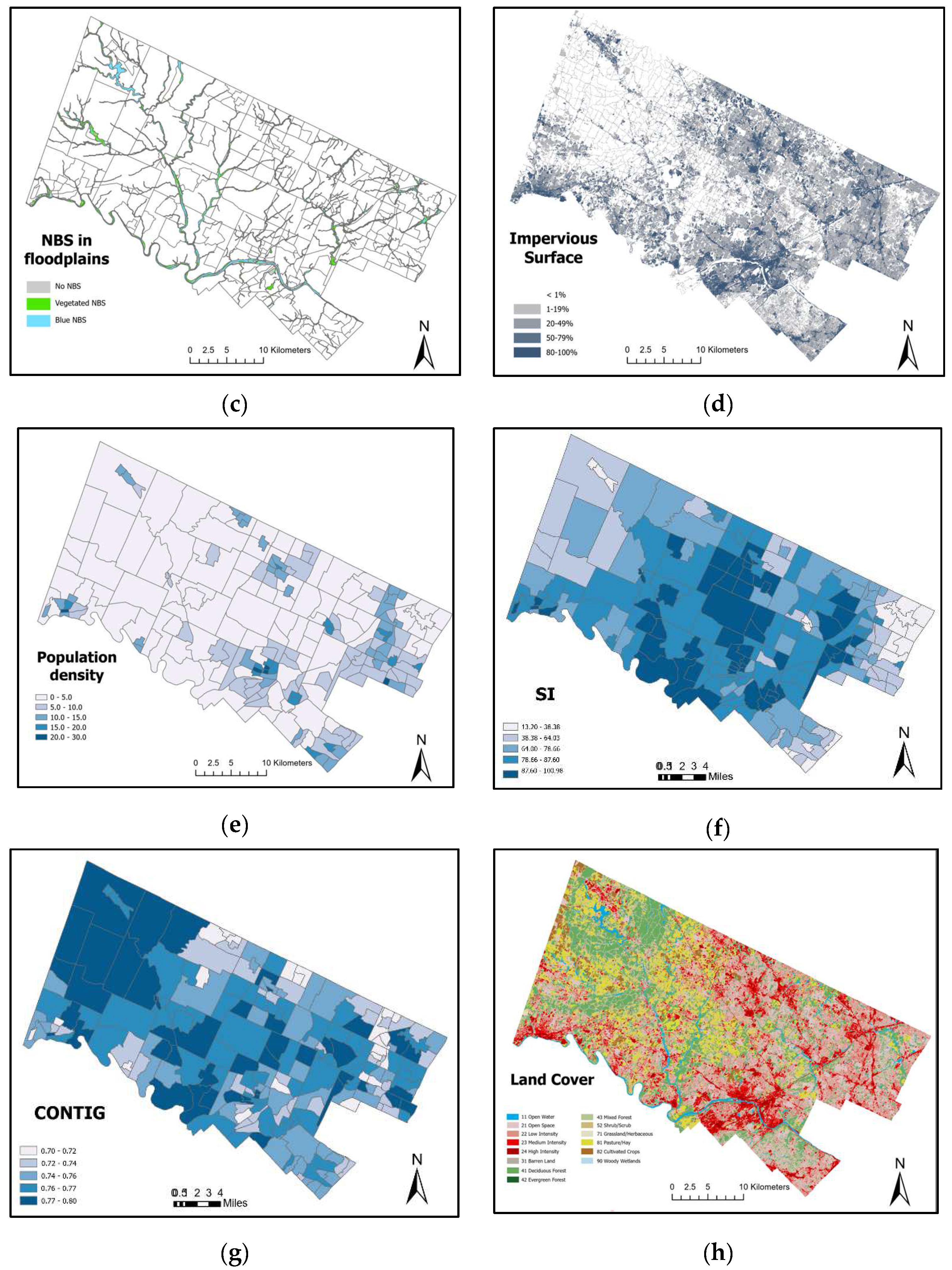
Table 3 presents the relationship between EALS and NBS and population density as per the GWR model. The overall R-square coefficient of determination nearly doubles in comparison to the GLR model, reaching a R2 of 0.44. The local R2 values in the GWR map range from 0.34 to 0.53. The higher local R2 values occurred in West Montgomery (Figure 3a). The lower AICc value and higher R2 suggests that GWR is more effective in identifying the local-scale association between EALS and independent variables. Furthermore, the analysis using Global Moran’s I test showed a significant clustering pattern in the standardized residuals (Moran’s I = 0.103; z score = 3.059).
When comparing the GLR model’s result for population density (PD) to GWR model, it becomes evident that the GWR model reveals more nuanced information, as depicted in Figure 3b. Surprisingly, a significant negative correlation between the PD and EALS was observed in 100.00% of the neighborhoods. The average GWR coefficient for this relationship was −0.312, with a standard deviation of 0.0318. It shows the smallest mean of GWR coefficients (−0.391). The influence of PD on EALS is particularly pronounced in the northern districts of the county. These findings suggest that the impact of population density on flood risk at a local scale is counterintuitive.
Regarding the amount of NBS in floodplains on a global scale, there is great evidence suggesting that a higher amount of NBS located within floodplains can increase the expected annual loss of flooding. Similarly, the GWR result demonstrates in all (100.00%) census tracts a positive significant relationship with ELAS. It is worth noting that this factor exhibits the highest mean of GWR beta coefficients (at 0.6244) compared to other variables. This disparity is particularly pronounced in a small part of East Montgomery. As one moves outward from this area to the west, the degree of association gradually decreases (refer to Figure 3c). In terms of impervious surface, in contrast to the global GLR model, the GWR model reveals a higher level of detail (see Figure 3d). It uncovers a significant positive correlation between the percentage of impervious surface and EALS in all census tracts (100.00%), with the mean GWR coefficient being 0.362 (SD = 0.029). The most significant association among the census tracts is observed in the southern part of the county, specifically in Upper Meridian Township, and as one moves to the left or right from this central area, the association diminishes, forming a distinct focal pattern.
In 21.90% of neighborhoods, a significant positive correlation was discovered between the CONTIG (contiguity) and EALS (expected annual loss score) variables. This finding suggests that higher connectivity among NBS patches can lead to an increase in the expected annual loss score from flooding. Specifically, the GWR analysis revealed an average coefficient of 0.235 with a standard deviation of 0.281. This relationship was particularly observed in the densely populated urban areas of Pottstown and Conshohocken cities (Figure 3e). Lastly, regarding the shape index (SI), there is no evidence that more complex shapes of NBS patches are associated with a lower or higher amount of EALS from both global and local perspectives. The highest level of association within the SI is concentrated in the northern districts of the county, gradually diminishing as we move outward from this central area (Figure 3f).
5. Discussion
The results of this study show that there is a strong positive association in all census tracts (100.00%) between each of the two variables of impervious surface and NBS size in floodplains with the expected annual loss of flooding in the study area, while population density significantly and negatively affects EALS. In contrast, the study findings reveal that irregular NBS patches show limited effectiveness in reducing total loss from flooding. Despite their presence, they do not yield a significant reduction in flood damage. However, the study uncovers a concerning trend with connected NBS patches in nearly one-fifth of the census tracts (21.90%), particularly in densely populated urban areas located in the southeast and southwest regions of the county. Surprisingly, the presence of connected NBS patches in these areas significantly amplifies the magnitude of flood loss, exacerbating the damage caused by flooding events.
One notable finding is the positive and statistically significant relationship between the percentage of impervious surface and EALS. The higher flood loss arises from the predominance of impervious surfaces within urban areas, which leads to increased surface runoff and places strain on the drainage system, consequently amplifying the risk of flood hazards. Therefore, it is crucial to consider incorporating “green” elements into gray infrastructure in urban areas across the county. This integration aims to mitigate the impact of impervious surfaces such as roads, buildings, and artificial facilities on flood risk. This finding aligns with previous research that has often observed an increase in flood risk and damage associated with higher levels of imperviousness [59].
Furthermore, the study results show a significant positive correlation between the size of NBS in floodplains and EALS, which is inconsistent with previous findings [18]. While scholarly evidence to support the physical basis of this causal relationship is lacking, a theoretical rationale is conceivable. According to the theory of Gilbert White (1945), which was referred to as the “levee effect,” the presence of more structural facilities like levees can lead to an increase in human activities and development in flood-prone areas. Similarly, an increase in vegetated areas in floodplains, while it may reduce population density and building construction, could lead to more agricultural and economic activities, which are considered in the EALS analysis. In other words, by having more accessible NBS in floodplains, with the tidal effects of rivers serving as the main source of irrigation, it is plausible that farmers may produce a greater quantity of crop products, which in turn might be at risk of flooding. Also, this result could be linked to the inadequate quality of NBS implementations and their lack of adaptability to the local ecosystem, leading to a heightened vulnerability of the natural environment to flooding risks [60]. Further research is warranted to investigate various types of NBS implemented in floodplains and to understand the intricate human–nature relationships unfolding in these regions, as observed in the case of Chenab River in Pakistan [61].
This study found a significant positive correlation between CONTIG and EALS, suggesting that NBS patterns featuring large contiguous and successive patches contribute to heightened total loss from flooding in some certain geographic locations, which is occupied by a denser development. The intensified impact of floods on immediate adjacent buildings loss may be attributed to the presence of larger interconnected nature-based solution (NBS) patches within dense urban areas, which influence the direction of surface water flow. Alternatively, this finding might be associated with the specific type of hydraulic conductivity between agricultural lands. It is plausible that the interconnected agricultural lands amplify the transfer of floodwater and debris flow to adjacent lands, thereby leading to increased damages (see O’Connell et al., 2007). Lastly, SI is a landscape metric providing information about the complexity and irregularity form of NBS, and a high value of SI indicates a more complex patch shape. Accordingly, there is no evidence showing a significant relationship between shape index and EALS in the study area, which is inconsistent with the results of recent studies [46,62], showing a relationship between the shape complexity of NBS with flood damage and vulnerability.
6. Conclusions
This study contributes to the existing knowledge by examining the complex spatial relationships between NBS and the expected annual loss score (EALS) of flooding in Montgomery County in Pennsylvania. Firstly, the primary focus is on addressing total property, agriculture, and population loss from flooding rather than simply considering insured claims which includes property damage. In addition, this research aims to explore the spatial heterogeneity of NBS in floodplains, NBS shape, and NBS contiguity through local spatial regression analysis by employing the GWR model, which offers a more comprehensive analysis compared to GLR model to uncover the spatial variations in NBS configuration and composition. By doing so, the areas with a high impact of NBS on flood loss reduction were identified.
The findings emphasize the significance of four key variables: population density, impervious surface, NBS size in floodplains, and CONTIG metric, which collectively account for approximately 45% of the variance in the expected annual loss score resulting from flooding. Although this may appear moderate, it aligns well with similar regression models that explain flood loss at the county jurisdictional level (as observed in Brody et al., 2007). The major results from this study are: (1) a higher amount of NBS in floodplains may have the negative impact on reducing the total damage from flooding; (2) more disconnected NBS patches effectively reduce the annual flood loss in denser areas; (3) lower percentage of impervious surface effectively decrease the annual loss of flooding; and (4) shape complexity of NBS patches does not affect flood loss. Results from the Generalized Linear Regression (GLR) and Geographically Weighted Regression (GWR) models also demonstrate non-stationarity in the relationship among these variables, with the GWR model exhibiting a superior model fit when compared to the GLR model.
While this study takes an important first step to consider the potential impact of NBS on total flood loss in one of the fastest growing counties in the U.S., further study is needed on the topic. First, it is important to note that while efforts were made to consider optimal parameters, there is still a possibility that certain parameters were not included in the models. Including additional socioeconomic and environmental variables as well as more landscape metrics and comparing their performances over time could further enhance the study. Second, future research should include variables quantifying specific characteristics of buildings and agricultural lands, such as size, type, building materials, degree of development, etc.- Third, I evaluated each metric at the census tract level due to the NRI availability in this level. Additional work should seek to overcome this limitation by examining different metrics at finer scales, particularly at the census block scale by using density-based approaches to downscale the data such as dasymetric mapping. Fourth, future investigations should look within specific urban areas and rural hinterlands to better contextualize the results of this more regional study. Finally, this study has focused on analyzing Montgomery County in the U.S. However, to obtain a more comprehensive understanding, further research should consider larger samples of counties or concentrate on more specific geographic areas for in-depth investigation.
Funding
This research received no external funding.
Data Availability Statement
The data presented in this study are available on request from the corresponding author.
Conflicts of Interest
The author declares no competing financial interest or personal relationships that could have appeared to influence the work reported in this paper.
References
- O’Donnell, E.C.; Thorne, C.R. Drivers of future urban flood risk. Philos. Trans. R. Soc. A 2020, 378, 3782019021620190216. [Google Scholar] [CrossRef]
- Pattison, I.; Lane, S.N. The link between land-use management and fluvial flood risk: A chaotic conception? Prog. Phys. Geogr. Earth Environ. 2012, 36, 72–92. [Google Scholar] [CrossRef]
- Venter, Z.S.; Krog, N.H.; Barton, D.N. Linking green infrastructure to urban heat and human health risk mitigation in Oslo, Norway. Sci. Total Environ. 2020, 709, 136193. [Google Scholar] [CrossRef]
- Zuniga-Teran, A.A.; Gerlak, A.K.; Mayer, B.; Evans, T.P.; Lansey, K.E. Urban resilience and green infrastructure systems: Towards a multidimensional evaluation. Curr. Opin. Environ. Sustain. 2020, 44, 42–47. [Google Scholar] [CrossRef]
- Tellman, B.; Sullivan, J.A.; Kuhn, C.; Kettner, A.J.; Doyle, C.S.; Brakenridge, G.R.; Erickson, T.A.; Slayback, D.A. Satellite imaging reveals an increased proportion of the population exposed to floods. Nature 2021, 596, 80–86. [Google Scholar] [CrossRef]
- IPCC. IPCC WGII Sixth Assessment Report: Chapter 6: Cities, Settlements and Key Infrastructure; IPCC: Geneva, Switzerland, 2021. [Google Scholar]
- National Weather Service. NWS Preliminary US Flood Fatality Statistics. 2022. Available online: https://www.weather.gov/arx/usflood (accessed on 9 August 2023).
- Wing, O.E.; Bates, P.D.; Smith, A.M.; Sampson, C.C.; Johnson, K.A.; Fargione, J.; Morefield, P. Estimates of present and future flood risk in the conterminous United States. Environ. Res. Lett. 2018, 13, 034023. [Google Scholar] [CrossRef]
- CoreLogic. Hurricane Report. 2021. Available online: https://www.preventionweb.net/publication/2021-hurricane-report (accessed on 23 July 2022).
- UN Habitat. Working for a Better Urban Future; UN Habitat: Nairobi, Kenya, 2018. [Google Scholar]
- Seto, K.C.; Güneralp, B.; RHutyr, L. Global forecasts of urban expansion to 2030 and direct impacts on biodiversity and carbon pools. Proc. Natl. Acad. Sci. USA 2012, 109, 16083–16088. [Google Scholar] [CrossRef]
- Chen, G.Z.; Li, X.; Liu, X.; Chen, Y.; Liang, X.; Leng, J.; Xu, X.; Liao, W.; Qiu, Y.; Wu, Q.; et al. Global projections of future urban land expansion under shared socioeconomic pathways. Nat. Commun. 2020, 11, 537. [Google Scholar] [CrossRef]
- Ferreira, C.S.S.; Kalantari, Z.; Hartmann, T.; Pereira, P. Conclusions. In Nature-Based Solutions for Flood Mitigation; Ferreira, C.S.S., Kalantari, Z., Hartmann, T., Pereira, P., Eds.; The Handbook of Environmental Chemistry; Springer: Cham, Switzerland, 2021; Volume 107. [Google Scholar]
- Hoyer, J.; Dickhaut, W.; Kronwitter, L.; Weber, B. Water Sensitive Urban Design: Principles and Inspiration for Sustainable Stormwater Management in the City of the Future; Jovis: Berlin, Germany, 2011. [Google Scholar]
- Samuels, P. The rise of natural flood management. J. Flood Risk Manag. 2022, 15, e12837. [Google Scholar] [CrossRef]
- Woodruff, S.; Bae, J.; Sohn, W.; Newman, G.; Tran, T.; Lee, J.; Wilkins, C.; Van Zandt, S.; Ndubisi, F. Planning, development pressure, and change in green infrastructure quantity and configuration in coastal Texas. Land Use Policy 2022, 114, 105893. [Google Scholar] [CrossRef]
- Razzaghi Asl, S.; Pearsall, H. How do Spatial Factors of Green Spaces Contribute to Flood Regulation in Urban Areas? A Systematic Mapping Approach. Prog. Phys. Geogr. Earth Environ. 2023, 47, 702–720. [Google Scholar] [CrossRef]
- Kim, M.; Song, K.; Chon, J. Key coastal landscape patterns for reducing flood vulnerability. Sci. Total Environ. 2021, 759, 143454. [Google Scholar] [CrossRef]
- Sakieh, Y. Understanding the effect of spatial patterns on the vulnerability of urban areas to flooding. Int. J. Disaster Risk Reduct. 2017, 25, 125–136. [Google Scholar] [CrossRef]
- Lallemant, D.; Hamel, P.; Balbi, M.; Ning Lim, T.; Schmitt, R.; Win, S. Nature-based solutions for flood risk reduction: A probabilistic modeling framework. One Earth 2021, 4, 1310–1321. [Google Scholar] [CrossRef]
- Latrubesse, E.M.; Park, E.; Sieh, K.; Dang, T.; Nina Lin, Y.; Yun, S.H. Dam failure and a catastrophic flood in the Mekong basin (Bolaven Plateau), southern Laos, 2018. Geomorphology 2020, 362, 107221. [Google Scholar] [CrossRef]
- Dottori, F.; Mentaschi, L.; Bianchi, A.; Alfieri, L.; Feyen, L. Cost-effective adaptation strategies to rising river flood risk in Europe. Nat. Clim. Chang. 2021, 13, 196–202. [Google Scholar] [CrossRef]
- IUCN. Position Paper for UNFCCC COP15, Copenhagen; IUCN: Gland, Switzerland, 2009. [Google Scholar]
- Prudencio, L.; Null, S. Stormwater management and ecosystem services: A review. Environ. Res. Lett. 2018, 13, 033002. [Google Scholar] [CrossRef]
- Brody, S.D.; Highfield, W.E.; Blessing, R.; Makinoc, T.; Shepard, C.C. Evaluating the effects of open space configurations in reducing flood damage along the Gulf of Mexico coast. Landsc. Urban Plan. 2017, 167, 225–231. [Google Scholar] [CrossRef]
- Castellar, J.A.C.; Popartan, L.A.; Pueyo-Ros, J.; Atanasova, N.; Langergraber, G.; Säumel, I.; Corominas, L.J.; Comas Acuña, V. Nature-based solutions in the urban context: Terminology, classification and scoring for urban challenges and ecosystem services. Sci. Total Environ. 2021, 779, 146237. [Google Scholar] [CrossRef]
- Zölch, T.; Henze, L.; Keilholz, P.; Pauleit, S. Regulating urban surface runoff through nature-based solutions—An assessment at the micro-scale. Environ. Res. 2017, 157, 135–144. [Google Scholar] [CrossRef]
- Kousky, C.; Walls, M. Floodplain conservation as a flood mitigation strategy: Examining costs and benefits. Ecol. Econ. 2014, 104, 119–128. [Google Scholar] [CrossRef]
- Sörensen, J.; Emilsson, T. Evaluating Flood Risk Reduction by Urban Blue-Green Infrastructure Using Insurance Data. J. Water Resour. Plan. Manag. 2019, 145, 04018099. [Google Scholar] [CrossRef]
- Brody, S.D.; Peacock, W.G.; Gunn, J. Ecological indicators of flood risk along the Gulf of Mexico. Ecol. Indic. 2012, 18, 493–500. [Google Scholar] [CrossRef]
- Bhattacharjee, K.; Behera, B. Does forest cover help prevent flood damage? Empirical evidence from India. Glob. Environ. Chang. 2018, 53, 78–89. [Google Scholar] [CrossRef]
- Forman, R.T.T. Some general principles of landscape and regional ecology. Landsc. Ecol. 1995, 10, 133–142. [Google Scholar] [CrossRef]
- Gill, S.E.; Handley, J.F.; Ennos, A.R.; Pauleit, S. Adapting cities for climate change: The role of green infrastructure. Built Environ. 2007, 33, 115–133. [Google Scholar] [CrossRef]
- Zhang, B.; Xie, G.; Li, N.; Wang, S. Effect of urban green space changes on the role of rainwater runoff reduction in Beijing, China. Landsc. Urban Plan. 2015, 140, 8–16. [Google Scholar] [CrossRef]
- Yao, L.; Chen, L.; Wei, W. Exploring the Linkage between Urban Flood Risk and Spatial Patterns in Small Urbanized Catchments of Beijing, China. Int. J. Environ. Res. Public Health 2017, 14, 239. [Google Scholar] [CrossRef]
- Lee, H.K. A panel data analysis of a spatial measurement of green infrastructure and its potential effectiveness on peak streamflow. Environ. Dev. Sustain. 2020, 22, 469–500. [Google Scholar] [CrossRef]
- Li, L.; Eetvelde, V.V.; Cheng, X.; Uyttenhove, P. Assessing stormwater runoff reduction capacity of existing green infrastructure in the city of Ghent. Int. J. Sustain. Dev. World Ecol. 2020, 27, 749–761. [Google Scholar] [CrossRef]
- Peng, Z.; Jinyan, K.; Wenbin, P.; Xin, Z.; Yuanbin, C. Effects of Low-Impact Development on Urban Rainfall Runoff under Different Rainfall Characteristics. Pol. J. Environ. Stud. 2019, 28, 771–783. [Google Scholar] [CrossRef]
- U.S. Census Bureau. Selected Population Characteristics, 2016–2020 American Community Survey 5-Year Estimates. 2020. Available online: http://factfinder2.census.gov/faces/tableservices/jsf/pages/productview.xhtml?pid=ACS_11_5YR_DP04 (accessed on 9 November 2023).
- Rossi, M.L.; Kremer, P.; Cravotta, C.A.; Scheirer, K.E.; Goldsmith, S.T. Long-term impacts of impervious surface cover change and roadway deicing agent application on chloride concentrations in exurban and suburban watersheds. Sci. Total Environ. 2022, 851, 157933. [Google Scholar] [CrossRef]
- Montgomery County Department of Emergency Services. Montgomery County Hazard Mitigation Plan; Montgomery County Department of Emergency Services: Norristown, PA, USA, 2022.
- The Reporter. Year in Review: Ida Leaves Mark in Montgomery County with Historic Flooding, Tornado Damage. 2021. Available online: https://www.thereporteronline.com/2021/12/31/year-in-review-ida-leaves-mark-on-montgomery-county-with-historic-flooding-tornado-damage/ (accessed on 17 July 2023).
- Kunkel, K.E.; Karl, T.R.; Squires, M.F.; Yin, X.; Stegall, S.T.; Easterling, D.R. Precipitation extremes: Trends and relationships with average precipitation and precipitable Water in the contiguous United States. J. Appl. Meteorol. Climatol. 2020, 59, 125–142. [Google Scholar] [CrossRef]
- FEMA. National Risk Index: Technical Documentation. 2023. Available online: https://www.fema.gov/sites/default/files/documents/fema_national-risk-index_technical-documentation.pdf (accessed on 6 November 2023).
- Zuzak, C.; Mowrer, M.; Goodenough, E.; Burns, J.; Ranalli, N.; Rozelle, J. The national risk index: Establishing a nationwide baseline for natural hazard risk in the US. Nat. Hazards 2022, 114, 2331–2355. [Google Scholar] [CrossRef]
- Sohn, W.; Bae, J.; Newman, G. Green infrastructure for coastal flood protection: The longitudinal impacts of green infrastructure patterns on flood damage. Appl. Geogr. 2021, 135, 102565. [Google Scholar] [CrossRef]
- Park, Y.; Guldmann, J.M. Understanding disparities in community green accessibility under alternative green measures: A metropolitan-wide analysis of Columbus, Ohio, and Atlanta, Georgia. Landsc. Urban Plan. 2020, 200, 103806. [Google Scholar] [CrossRef]
- Bai, T.; Mayer, A.L.; Shuster, W.D.; Tian, G. The Hydrologic Role of Urban Green Space in Mitigating Flooding (Luohe, China). Sustainability 2018, 10, 3584. [Google Scholar] [CrossRef]
- Kim, H.W.; Park, Y. Urban green infrastructure and local flooding: The impact of landscape patterns on peak runoff in four Texas MSAs. Appl. Geogr. 2016, 77, 72–81. [Google Scholar] [CrossRef]
- McGarigal, K. FRAGSTATS Help; University of Massachusetts: Amherst, MA, USA, 2015. [Google Scholar]
- McCullagh, P.; Nelder, J.A. Generalized Linear Models, 2nd ed.; CRC Press: Boca Raton, FL, USA, 1989. [Google Scholar]
- Pearsall, H.; Christman, Z. Tree-lined lanes or vacant lots? Evaluating non-stationarity between urban greenness and socio-economic conditions in Philadelphia, Pennsylvania, USA at multiple scales. Appl. Geogr. 2012, 35, 257–264. [Google Scholar] [CrossRef]
- Jongman, B.; Ward, P.J.; Aerts, J.C.J.H. Global exposure to river and coastal flooding: Long-term trends and changes. Glob. Environ. Chang. 2014, 22, 823–835. [Google Scholar] [CrossRef]
- Brody, S.D.; Highfield, E. Open space protection and flood mitigation: A national study. Land Use Policy 2013, 32, 89–95. [Google Scholar] [CrossRef]
- Anselin, L. Spatial econometrics. In Methods and Models; Kluwer Academic Publishers: Dordrecht, The Netherlands, 1988. [Google Scholar]
- Fotheringham, A.; Brunsdon, C.F.; Charlton, M. Geographically Weighted Regression: The Analysis of Spatially Varying Relationships; John Wiley & Sons: West Sussex, UK, 2002. [Google Scholar]
- Brundson, C.; Fotheringham, A.S.; Charlton, M. Geographically weighted regression: A method for exploring spatial non-stationarity. Geogr. Anal. 1996, 28, 281–298. [Google Scholar]
- Bagstad, K.J.; Villa, F.; Johnson, G.W.; Voigt, B. ARIES (Artificial Intelligence for Ecosystem Services) v2.1. User Guide and Technical Documentation; The Nature Conservancy: Arlington, VA, USA; Conservation Biology Institute: Corvallis, OR, USA; World Wildlife Fund: Morges, Switzerland, 2013. [Google Scholar]
- Brody, S.D.; Zahran, S. Examining the impact of the built environment on flood losses in Texas. WIT Trans. Ecol. Environ. 2007, 102, 389–398. [Google Scholar]
- Seddon, N.; Chausson, A.; Berry, P.; Girardin, C.A.J.; Smith, A.; Turner, B. Understanding the value and limits of nature-based solutions to climate change and other global challenges. Philos. Trans. R. Soc. B 2020, 375, 20190120. [Google Scholar] [CrossRef]
- Tariq, M.A.; Rajabi, Z.; Muttil, N. An Evaluation of Risk-Based Agricultural Land-Use Adjustments under a Flood Management Strategy in a Floodplain. Hydrology 2021, 8, 53. [Google Scholar] [CrossRef]
- Kim, H.Y. Analyzing green space as a flooding mitigation—Storm Chaba case in South Korea. Geomat. Nat. Hazard Risk 2021, 12, 1181–1194. [Google Scholar] [CrossRef]
Figure 1.
Study area of Montgomery County, Pennsylvania, USA with delineated Schuylkill River, local creeks, and subregions.
Figure 1.
Study area of Montgomery County, Pennsylvania, USA with delineated Schuylkill River, local creeks, and subregions.
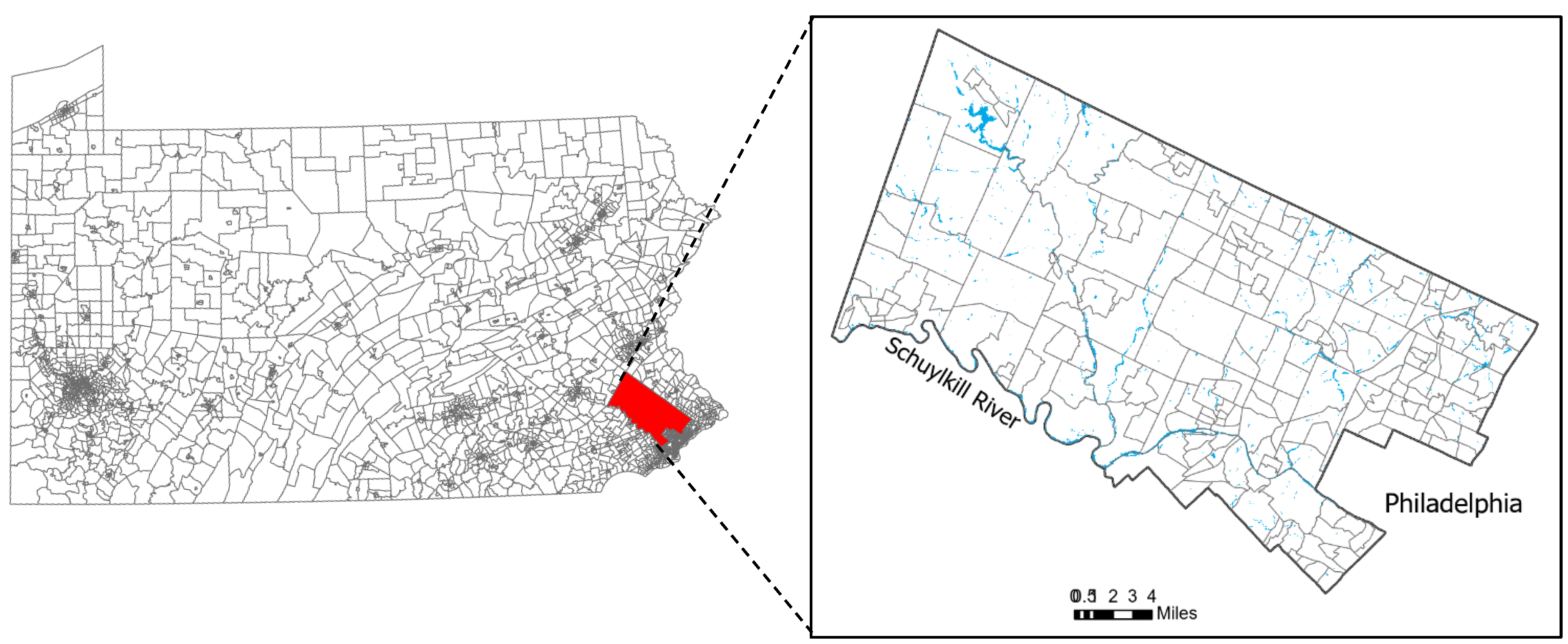
Figure 2.
NBS and Impervious surfaces distribution in study area, including (a) Expected Annual Loss Score, (b) NBS distribution in the whole study area, (c) NBS distribution in 100-year flood zone area distribution, (d) Impervious surface percentage in study area, (e) Population density, (f) Shape index, (g) Contiguity index, and (h) Land cover map.
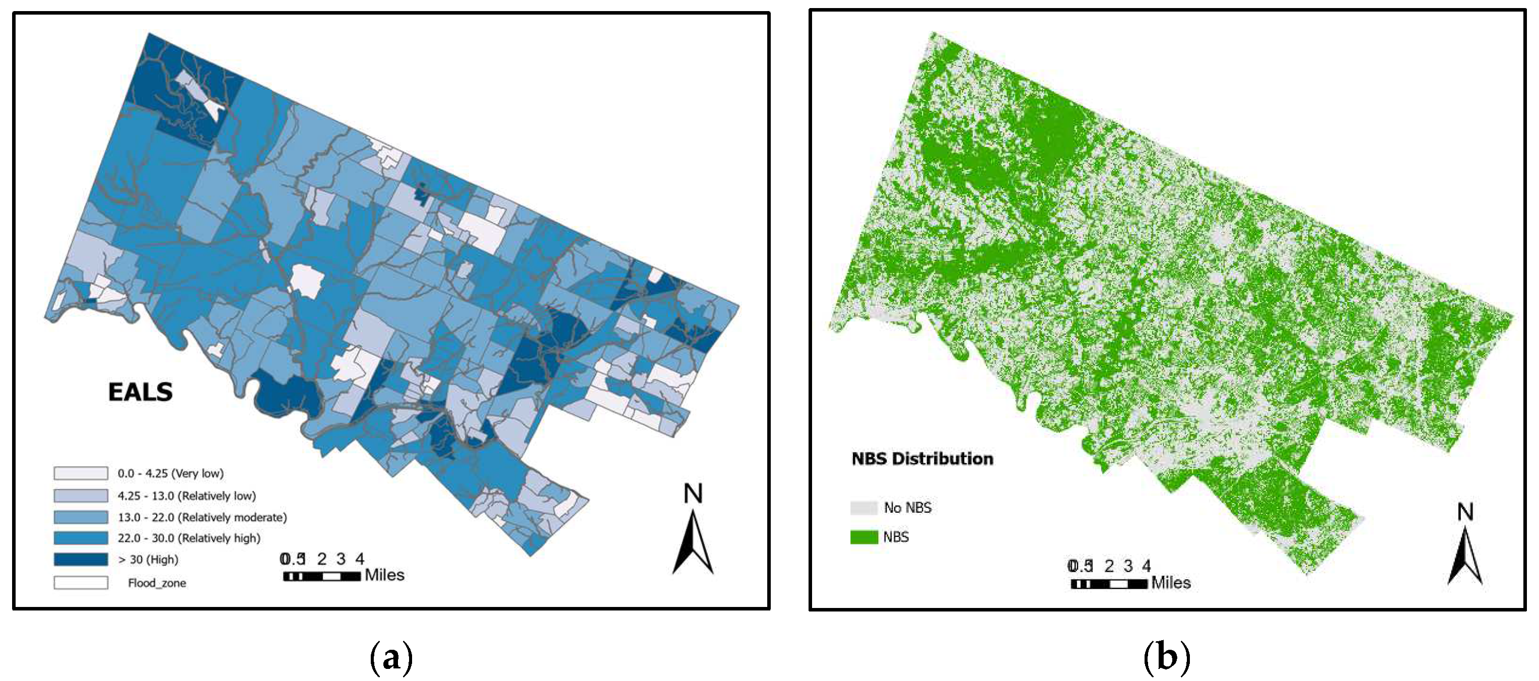

Figure 3.
Spatially explicit GWR results, including (a) Local R2, (b) GWR coefficient, population density, (c) GWR coefficient, NBS in floodplains, (d) GWR coefficient, impervious surface percent, (e) GWR coefficient, contiguity index, and (f) GWR coefficient, shape index.
Figure 3.
Spatially explicit GWR results, including (a) Local R2, (b) GWR coefficient, population density, (c) GWR coefficient, NBS in floodplains, (d) GWR coefficient, impervious surface percent, (e) GWR coefficient, contiguity index, and (f) GWR coefficient, shape index.


Table 1.
Datasets and main variables.
| Variable | Source | Range | Mean |
|---|---|---|---|
| Dependent variable Expected Annual Loss Score (EALS) | National Risk Index dataset for flooding | 0~38 | 13.4 |
| Independent variables NBS in floodplains (NBSF) area (km2) Impervious area (IA) percentage Shape index (SI) Contiguity index (CONTIG) Control variable Population density (per acre) (PD) | National Flood Hazard Layer (NFHL) NLCD 2019 NLCD 2019 NLCD 2019 U.S. census tract data | 0~3.2 1.83~74.1 13.2~100.98 0.7~0.8 0.31~30.32 | 0.31 27.7 74 0.75 5.55 |
Table 2.
Results of Generalized Linear Regression (GLR) model for Expected Annual Loss Score.
| Variable | Coefficient | Robust SE | Robust t | Robust P | VIF | Moran’s I |
|---|---|---|---|---|---|---|
| Intercept | −44.44 | 19.07 | −2.32 | 0.020 | --- | ---- |
| NBSF | 6.428 | 1.264 | 5.083 | 0.000 * | 1.504 | 0.21 * |
| IA | 0.175 | 0.059 | 2.961 | 0.0034 * | 2.823 | 0.402 * |
| SI | −0.018 | 0.0242 | −0.780 | 0.435 | 1.071 | 0.598 * |
| CONTIG | 72.587 | 24.892 | 2.915 | 0.0039 * | 1.244 | 0.297 * |
| PD | −0.451 | 0.148 | −3.046 | 0.0026 * | 1.996 | 0.299 * |
| Model Diagnostics | ||||||
Note: SE = standard error; VIF = variance inflation factor. * Significant at the 0.01 level. Multiple R2: 0.240, adjusted R2: 0.222, AICc: 1399.10, Koenker (BP): 30.952 *, Jarque-Bera: 5.590 *.
Table 3.
Local-scale association between Expected Annual Loss Score and NBS status based on the GWR model.
Table 3.
Local-scale association between Expected Annual Loss Score and NBS status based on the GWR model.
| Variable | GWR Coefficients | Directions of Relationship in the GWR Model | ||||||
|---|---|---|---|---|---|---|---|---|
| Min | Max | Mean | SD | + (%) | +sig. (%) | − (%) | −sig. (%) | |
| Intercept | 0.2085 | 0.3209 | 0.1337 | 0.1672 | --- | --- | --- | --- |
| NBSF | 0.3087 | 1.0887 | 0.6244 | 0.2090 | 100.00% | 100.00% | 0.00% | 0.00% |
| IA | 0.2856 | 0.4167 | 0.3624 | 0.0294 | 100.00% | 100.00% | 0.00% | 0.00% |
| SI | −0.1718 | −0.0309 | −0.1015 | 0.0313 | 0.00% | 0.00% | 100.00% | 00.00% |
| CONTIG | 0.3387 | 1.0227 | 0.2353 | 0.2816 | 80.00% | 21.90% | 20.00% | 0.00% |
| PD | −0.3912 | −0.2416 | −0.312 | 0.0318 | 0.00% | 0.00% | 100.00% | 100.00% |
| Model Diagnostics | ||||||||
Note: +sig. (%) and −sig. (%) refer to the proportion of 5% significance for positive correlation and negative correlation, respectively. Multiple R2: 0.442, adjusted R2: 0.372, AICc: 530.865, Moran’s I: 0.103.
Disclaimer/Publisher’s Note: The statements, opinions and data contained in all publications are solely those of the individual author(s) and contributor(s) and not of MDPI and/or the editor(s). MDPI and/or the editor(s) disclaim responsibility for any injury to people or property resulting from any ideas, methods, instructions or products referred to in the content. |
© 2023 by the author. Licensee MDPI, Basel, Switzerland. This article is an open access article distributed under the terms and conditions of the Creative Commons Attribution (CC BY) license (https://creativecommons.org/licenses/by/4.0/).
Share and Cite
MDPI and ACS Style
Razzaghi Asl, S. To What Extent Have Nature-Based Solutions Mitigated Flood Loss at a Regional Scale in the Philadelphia Metropolitan Area? Urban Sci. 2023, 7, 122. https://doi.org/10.3390/urbansci7040122
AMA Style
Razzaghi Asl S. To What Extent Have Nature-Based Solutions Mitigated Flood Loss at a Regional Scale in the Philadelphia Metropolitan Area? Urban Science. 2023; 7(4):122. https://doi.org/10.3390/urbansci7040122
Chicago/Turabian StyleRazzaghi Asl, Sina. 2023. "To What Extent Have Nature-Based Solutions Mitigated Flood Loss at a Regional Scale in the Philadelphia Metropolitan Area?" Urban Science 7, no. 4: 122. https://doi.org/10.3390/urbansci7040122