Machine Learning Methods in CFD for Turbomachinery: A Review

Abstract

Computational Fluid Dynamics is one of the most relied upon tools in the design and analysis of components in turbomachines. From the propulsion fan at the inlet, through the compressor and combustion sections, to the turbines at the outlet, CFD is used to perform fluid flow and heat transfer analyses to help designers extract the highest performance out of each component. In some cases, such as the design point performance of the axial compressor, current methods are capable of delivering good predictive accuracy. However, many areas require improved methods to give reliable predictions in order for the relevant design spaces to be further explored with confidence. This paper illustrates recent developments in CFD for turbomachinery which make use of machine learning techniques to augment prediction accuracy, speed up prediction times, analyse and manage uncertainty and reconcile simulations with available data. Such techniques facilitate faster and more robust searches of the design space, with or without the help of optimization methods, and enable innovative designs which keep pace with the demand for improved efficiency and sustainability as well as parts and asset operation cost reduction.

1. Introduction

Turbomachines, and in particular Gas Turbines (GT), have been widely used in the last decades for propulsion, both aviation and marine, power generation and mechanical drive; while Steam Turbines (ST) have been used mostly for large scale power generation, both standalone and in conjunction with GT in combined cycles [1]. GT technology is nearing maturity and efficiency, reliability, availability, and operating range are now close to entitlement. Consequently, further improvement becomes increasingly complex and expensive. Most of these units are fossil fuels fired, and the increasing pressure to reduce their carbon footprint [2] calls for changes that require innovations in many technology areas to drastically reduce, or zero, emissions and interface seamlessly with renewable resources. Some examples to cite a few are:

• Fuel flexibility (methane, hydrogen, ammonia, oxi-combustion, and a blend of these with low NO${}_x$ emissions),
• Part load performance (when operating below 50% of nominal power),
• Fast start-up and shut-down (which should take less than a minute to allow interfacing with intermittent renewables),
• Better efficiency (higher firing temperatures and pressures and improved materials properties),
• Reduced maintenance (for operation in remote areas close to wind or solar farms),
• Improved interface with bottom cycles (operated with steam or organic fluids),
• Interfacing with Carbon Capture and Sequestration (CCS).

Consequently, designers are faced with the prospect of moving away from well-established comfort-zone designs, either by applying conventional design to uncharted applications, or by designing new units in uncharted design spaces [3]. All of these challenge the entire design process, from the early conceptual to the preliminary and detailed design stages.

In the specific areas of aerodynamics, aeromechanics (both forced response and flutter), heat transfer, and combustion, design systems are evolving from correlation-based designs, relying heavily on companies’ proprietary experimental data, to more complex multidimensional and multidisciplinary approaches that require Computational Fluid Dynamics (CFD) [3,4]. Correlation-based designs are naturally bound to the investigated design space envelope and are not suited for exploring design opportunities outside this space. As a more complex design verification tool based on first principles, CFD has the potential to investigate any design space. Unfortunately, conventional CFD such as steady and unsteady Reynolds-averaged Navier–Stokes (RANS and URANS), which are the main subject of this paper, also suffer from fundamental weaknesses. These can be imputed primarily to turbulence and heat transfer models, and secondly to the geometry and operating condition simplifications often made to reduce the computational effort [5,6]. To overcome such deficiencies, most companies develop so-called “best practices” to run CFD and minimize the deviation from measured data, which apply only to the design space in which reliable data are available. Consequently, conventional CFD reliability as a general design tool, although much more powerful compared to correlation-based and simple 1D and 2D methods, is undermined and design safety margins are applied as a measure of the “ignorance” of designers and the tools [6].

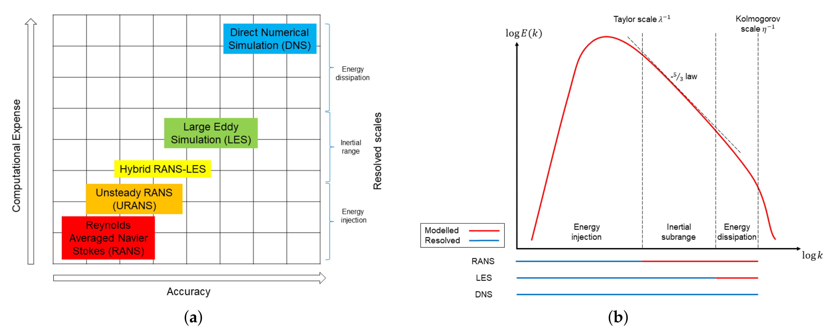
In previous years, scale resolving simulations such as Large Eddy Simulation (LES) and Direct Numerical Simulation (DNS), as opposed to time-averaging methods like (U)RANS, emerged as a viable design aid (see, for example, applications to low-pressure turbines [7,8,9], and combustion systems [10]). Figure 1a shows where each method lies on the trade-off between accuracy and computational expense and Figure 1b shows the correlation of these methods to the energy spectrum. LES resolves the majority of the fluid flow energy spectrum and models only the finer dissipation scales where the assumption of quasi-isotropic turbulence is acceptable [11]. Despite their undeniable superiority to (U)RANS, LES with appropriate grid resolution is still computationally prohibitive for wall-driven and statistically periodic flows such as those in multistage compressors and turbines, while it is more common for the wall-bounded and statistically steady flows present in combustion chambers [12]. Scale resolving simulations offer superior resolution allowing designers to determine not only what is happening in the fluid flow, but also why it is happening [6,11]. This distinction has unlocked an alternative use of scale resolving simulations as accurate datasets to benchmark and improve (U)RANS models. It is important to remember that the most popular two-equation model, k-$ϵ$ [13], was originally developed and calibrated for boundary layers and free jet flows, and has since been applied with a fair degree of accuracy to much more complex flows. Therefore, LES and DNS provide the perfect databases to improve lower-order models, especially when using different forms of machine learning (ML).

Improved (U)RANS predictability, as well as both Hybrid-LES (HLES) and LES in narrower application ranges, allows the design space to be extended with less fear of running into inaccurate predictions. A potential by-product of such improvement is represented by design optimization methods, from simple airfoils aero and aeromechanics [14], to more advanced multidimensional topology optimization [15] that can ultimately be used with more confidence while overcoming the excessive computational effort of scale-resolved simulations. With this premise, this paper attempts to describe current research activities to evolve CFD methods with the aid of high-fidelity simulation and ML, to further improve accuracy in both academic and industrial applications.

2. Application of Machine Learning Methods to CFD for Turbomachinery Design

The accurate prediction of flow fields is key to the development of new technologies and products in the critical early phase where a wide design space needs to be explored. Such necessity does not apply only to turbomachines, but to each application in which a fluid flow is required to store or convert various forms of energy into various forms of power. Industry, more than academia, has always faced the challenge of handling heterogeneous datasets with varying levels of fidelity. These range from simple scaled-down tests, to full-scale full-system tests, as well as field data from the results of associated computational design tools. Moreover, the quality of both experimental and computational tools is continuously improving (for example advanced ceramic probes for high-pressure high-temperature flows, or LES with appropriate discretization for real geometries and operating conditions) as is the cost of running experiments and high-fidelity simulations. Given the sheer size of the heterogeneous datasets present in industry, an updated engineering approach based on ML methods is required to leverage the available data efficiently. With an eye on the application of improved prediction methods, several key avenues currently being explored to various extents, but which nevertheless are worthy of due consideration, are described below:

• How can ML indicate ways to improve accuracy at various levels of physics resolution? With reference to Figure 1a, DNS can be used to improve the subgrid-scale (SGS) model in LES, which can be used to improve Reynolds-averaged models in (U)RANS. In particular, we focus on Artificial Neural Networks (ANNs) and Gene Expression Programming (GEP) based methods that use data from DNS or LES to improve the accuracy of (U)RANS in some respect.
• Are ML methods a viable strategy for reduction of computational cost associated with a single CFD simulation by accelerating the convergence of solvers?
• Uncertainty quantification (UQ) is employed during the design of new products to determine the impact of different sources of uncertainty on the performance of a design. Computing the statistical moments of an uncertain Quantity of Interest (QoI) does not generally admit analytical solutions, but instead requires meta-models that are not only accurate but can scale well with the number of uncertain system parameters. These models must also be able to handle large, heterogeneous datasets containing data with varying levels of uncertainty. Furthermore, the results of the uncertainty analysis must be clearly communicated to multi-disciplinary teams who are stakeholders in the project. How can ML based methods be used to address these challenges?
• Finally, is the model able to incorporate multi-fidelity data and help match scarce experimental measurements affected by errors? Is the model generalisable to a range of flow features (for instance adverse or favourable pressure gradients), geometries (wall-bounded vs. wall-driven) and flow conditions (statistically steady vs. statistically periodic)?

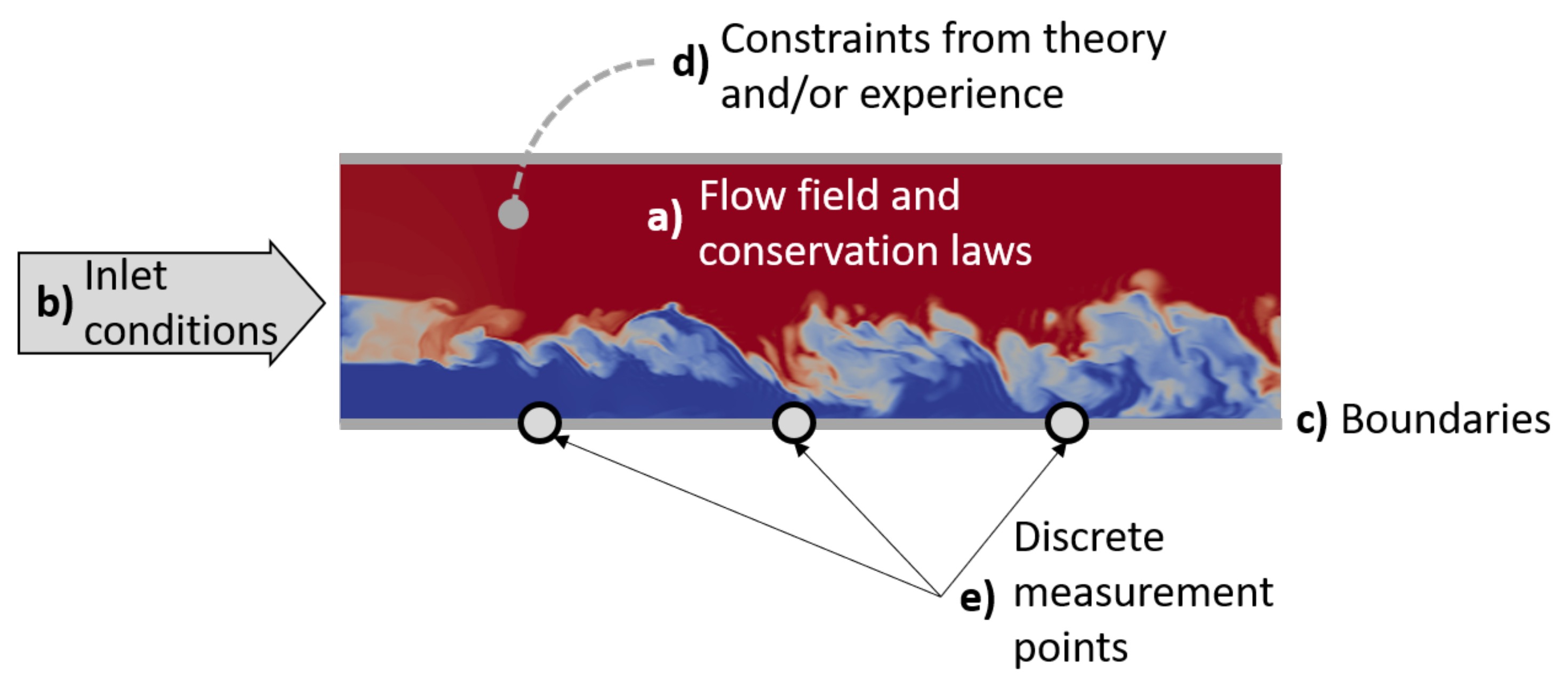
To facilitate the discussion of these points, reference is made to Figure 2, showing an instantaneous snapshot of the thermal field in proximity to the trailing edge of a high-pressure turbine (HPT). The figure summarizes the different sets of information available, including the flow field computed employing CFD methods with different levels of resolution.

3. Turbulence Modeling with Machine Learning

The modelling of turbulence effects in the internal flows of turbomachines is particularly complex due to the interaction of a wide range of frequencies and the associated flow structures. Although captured sufficiently in simple cases by classical (U)RANS methods, regions of high anisotropy and wide ranges of interacting length scales cause the inherent assumptions relied upon in the development of the RANS closures to break down. The aim of machine learning in this context is to improve the accuracy of CFD calculations without resorting to high-fidelity, scale resolving and computationally expensive techniques. This simple premise has driven the development of a vast range of techniques over the last 10 years each underpinned by a simple philosophy; use data generated from experiments and, mostly, from high-fidelity simulations to inform on uncertainty and corrections to existing LES, HLES, and (U)RANS data, and eventually to develop improved models.

In this scenario, with reference to Figure 2, the flow field $\left(a\right)$ is available from high-fidelity simulations with a good degree of accuracy, as well as inlet conditions $\left(b\right)$ and boundaries $\left(c\right)$ while discrete measurements points, $\left(e\right)$, may be available only to validate the high-fidelity data. The constraints from theory, $\left(d\right)$, are generally considered in the model learning phase. Approaches can then be largely split into two distinct categories:

• Those that find corrective functions for the Reynolds stress or other quantities of interest and apply these in one predictive step to the baseline model. This involves introducing the corrected Reynolds stress into lower-order closures (DNS to LES or HLES, and LES to (U)RANS) as a static field from which the velocity and pressure field can be converged.
• Those that make inherent changes to lower-order closures (mostly (U)RANS), either through terms in the turbulence equations or by learning nonlinear models for the Reynolds stresses based on mean flow features, as discussed in [16]. These models are then inferenced at every iteration in a subsequent (U)RANS calculation.

Each approach has merits and deficiencies although it is considered that, at convergence, they both yield similar results. Methods using the first approach can learn discrepancies and make corrections to the quantity of interest in an environment completely removed from CFD. Just one additional solver is required to predict the mean flow variables which solves the RANS equations injected with a static Reynolds stress field. This modularity keeps implementation simpler and allows the CFD engineer and the machine learning engineer to operate individually. The second approach requires the machine learning and the RANS calculations to be more intrinsically linked [17]. As the model must be inferenced at every step, the machine learnt model must be implemented in the RANS solver. This can introduce a significant amount of overhead code as different models may need different implementations. However, once developed, the model is self-contained and can be run independently.

3.1. The Energy Spectrum in Turbomachinery

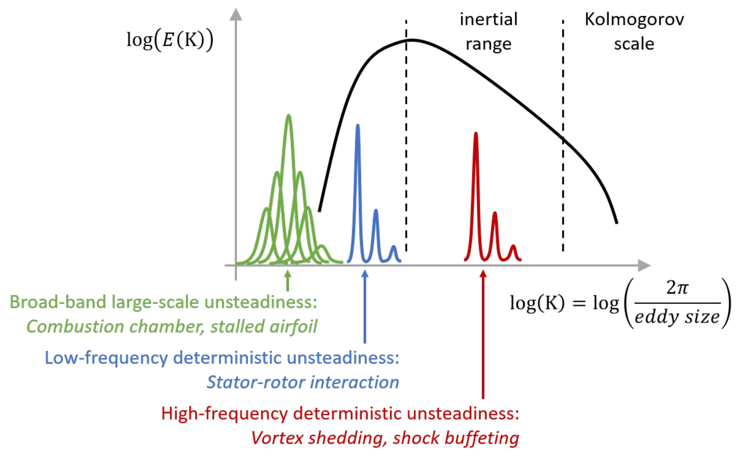
Figure 3 illustrates the typical energy plot as a function of the wavenumber $\left(K\right)$ for homogeneous turbulence. The solid black line shows a peak that corresponds to the maximum energy eddies that, moving to the right, progressively transfer energy to smaller eddies down to the Kolmogorov scale at which viscous dissipation becomes dominant. Figure 4 sketches the range of different modelling paths, which will be illustrated with the help of Figure 3.

3.2. DNS to Improve LES

A well-resolved DNS constitutes a formidable dataset to develop turbulence models as it resolves the majority of the Kolmogorov scales at which turbulence is substantially isotropic. The resolution in LES in terms of K sits in the inertial scale range, as close as possible to the Kolmogorov scale limit to minimize the importance of the SGS model. While the open literature offers a wide range of models [18], a good example of the development of an SGS model with the help of ML based on a DNS database is described by Park and Joi [19], who used a Neural Network trained on a DNS of a $R{e}_{\tau }=178$ flow. They proved that the resulting SGS model could be applied to channel flows at much larger Reynolds numbers. With reference to Figure 4, this is the branch A in which the conservation of a generic quantity f requires the introduction of the additional SGS term in its transport equation

$$\frac{Df}{Dt}=\underset{\mathrm{resolved}}{\underbrace{\frac{\partial f\left(\mu ,▿f_i\right)}{\partial x_j}}}+\underset{\mathrm{SGS} \mathrm{spatial} \mathrm{average}}{\underbrace{\frac{\partial f\left({\mu }_{\mathrm{SGS}},▿f_i\right)}{\partial x_j}}}.$$

(1)

In case the resolution in space and time is enough for DNS, the diffusion process depends on the viscosity $\mu$, which is a fluid property. When the resolution is not enough, it is necessary to introduce the SGS viscosity ${\mu }_{\mathrm{SGS}}$ that is a flow property averaged over the length scale of the spatial grid resolution.

3.3. DNS and LES to Improve HLES

Branch B covers the so-called hybrid-LES (HLES) approach in which models switch to RANS where the grid resolution in space is insufficient. This approach requires cumbersome interfacing of LES, which is a space-averaged method, with RANS, which is a time-averaged method. Weatheritt and Sandberg [20] used machine learning, in particular Gene Expression Programming (GEP), to tune their HLES approach with the help of a companion LES and obtained very encouraging results for the flow past twin cylinders.

3.4. DNS and LES to Improve (U)RANS

Potentially the most common path by which machine learning has been employed in CFD to date is via inference of (U)RANS turbulence closures from higher-fidelity DNS and LES databases. To this end, Weatheritt and Sandberg [21] developed a novel form of GEP capable of regressing tensorial expressions. As a symbolic regression technique, GEP provides explicit algebraic expressions for the quantity of interest which in this case is the anisotropy. Using the explicit algebraic Reynolds stress (EASM) framework of Pope [22], they learnt improved nonlinear expressions for the anisotropy which showed promise in predictive circumstances where the included physics is similar. The GEP methodology has since been applied to flows relevant in the turbomachinery space, looking at the HPT cascade [23] and extended the approach to develop nonlinear scalar-flux models for heat transfer analysis by developing a general form of the scalar-flux based on functional dependence [24]. Applying GEP to LES data of a jet in crossflow representative of film cooling techniques, they observed significant improvement in the prediction of the scalar-flux term, culminating in adiabatic effectiveness values more accurately reproducing experiments for a range of blowing ratios.

Hammond et al. [25] looked to further the GEP methodology introduced by Weatheritt and Sandberg to validate its capability on more complex 3D flows, such as those generated by topology optimisation. Using a topology optimised heat exchanger duct as a test case for a complex internal cooling system, they showed an improved assessment of the aerodynamic blockage when compared to DES reference data. This analysis is performed with the intention of applying data-driven closures in fluid optimisation methods, to achieve designs representative of high-fidelity flow prediction at a fraction of the computational cost. Whilst GEP has the merit of providing the user with an explicit expression which can be easily assimilated and assessed, the functional forms that can be expressed are sometimes limited. ANNs provide the option of greater flexibility and are potentially able to perform wider searches of the parameter space. Frey et al. [26] built on the work of Ling et al. [27] and used relatively shallow neural networks trained on DNS data to improve the eddy viscosity term in the Boussinesq approximation. They applied this approach to a serpentine channel representative of internal cooling channels in turbine blades. Using a hierarchical agglomerative clustering algorithm to separate regions of the flow for training, they showed that improved results were achieved when the separation regions around each bend were excluded from training. This was attested to the importance of accurately predicting turbulent mixing in the flow preceding the separation point and just outside the rear part of the bubble.

Therefore, ML can be used to develop Reynolds-averaged models using LES (and DNS when available) by using both different forms of ANNs and GEP, as discussed in [28]. However, different ways to evaluate the fit of the model when introduced in RANS [17] may also be explored, as summarized in Figure 5. Zhao et al. [17] observed that it was convenient to verify the trained ${\tau }_{i,j}^{ML}$ by using the updated flow field resulting from a new RANS calculation with the latest candidate constitutive flow as opposed to testing it with the frozen velocity field from LES. Obviously, the training effort increases significantly, but it overcomes the problems of the nonlinear response of the NS equations to changes in the constitutive law.

Additionally, as turbomachinery flows are inherently unsteady, it is necessary to distinguish between RANS and URANS. In this class of models, fine-scale high frequency motion effects are entirely filtered out and replaced with the so-called Reynolds-stresses that apply to both turbulent diffusion of momentum and thermal energy.

The filtering process assumes a canonical spectrum, similar to the black line in Figure 3 representative of isotropic turbulence decay. In turbomachines, the energy spectrum may change due to several possible reasons listed in Figure 3. Combustion systems generate “broad-band” large-scale unsteadiness that alters the fundamental process of extracting energy from the mean flow field, and large-scale flow structures are also generated in axial compressors and turbines post-stall. In this case, RANS may be accurate as long as the broad-band low frequency energy is small, although it is unclear if the Reynolds-averaging process based on the canonical spectrum will still work, and an unsteady RANS that resolves the low frequencies may be a better choice. This is represented by branches C and D in Figure 4. The energy spectrum of Figure 3 may also change due to the large scale “deterministic” unsteadiness generated by stator–rotor interaction, trailing edge vortex shedding, and shock buffeting.

Stator–rotor interaction is driven by the blade-passing frequency that depends on the airfoil count and the rotational speed, and it generally sits outside the inertial range. Therefore, the so-called spectral gap (the gap between the deterministic frequency and the frequency range that defines the inertial range) is preserved and the Reynolds-averaging process is appropriate [11,29]. In spite of the spectral gap, complex constitutive laws may still be required to capture the airfoil–wake interaction, as documented by Michelassi et al. [30] due to curvature and pressure gradient effects. This scenario is represented by branches E and F in Figure 4.

With high frequencies, like in high-pressure turbine trailing edge vortex shedding or in supersonic flows with shock buffeting, the deterministic contribution may sit inside the inertial range and the spectral gap vanishes. Consequently, there is a strong interaction between the deterministic unsteadiness and the turbulence energy cascade. In this scenario, Reynolds-averaging will wrongly filter the deterministic contribution, and it will fail (branches E and F). In this case, the conservation of a generic quantity f can be formulated as

$$\frac{Df}{Dt}=\underset{\mathrm{laminar}}{\underbrace{\frac{\partial f\left(\mu ,▿f_i\right)}{\partial x_j}}}+\underset{\mathrm{Reynolds} \mathrm{average}}{\underbrace{\frac{\partial f\left({\mu }_t,▿f_i\right)}{\partial x_j}}}.$$

(2)

Similarly to Equation (1), the molecular viscosity $\mu$ depends on the fluid, while the turbulent viscosity ${\mu }_t$ is a flow property averaged in time.

To overcome the difficulties that a turbulence model has to mimic both deterministic and stochastic unsteadiness, Akolekar et al. [7] and Lav et al. [31] adopted different approaches. In [7], the authors applied GEP to develop a RANS turbulence closure based on several phase-locked averaged flow fields from the LES of a low-pressure turbine with discrete incoming wakes. The results showed a substantial improvement compared to a standard two-equation model, although the gap with LES was still evident. In [31], the authors used the LES past an infinite plate to reproduce the vortex shedding typical of a low-pressure turbine. The developing wake has both large stochastic unsteadiness (i.e., turbulence) and large coherent unsteadiness due to the shedding of discrete vortices. The authors proposed a triple decomposition in which the flow field is split into a steady time-averaged flow, a periodic component extracted by FFT, and a stochastic component in a way similar to the so-called Partially-Averaged Navier–Stokes (PANS) equations. They concluded that the best match with LES was obtained by running URANS with a turbulence model trained only on the stochastic component of the LES flow field.

In the past, Van de Wall et al. [32] extended the Reynolds stresses that model the effect of stochastic unsteadiness due to turbulence on the mean flow field, to the so-called deterministic stresses meant to model the effect of deterministic unsteadiness due to stator–rotor interaction on the mean flow field, represented by branch G in Figure 4. Therefore, the resulting conservation equation becomes

$$\frac{Df}{Dt}=\underset{\mathrm{laminar}}{\underbrace{\frac{\partial f\left(\mu ,▿f_i\right)}{\partial x_j}}}+\underset{\mathrm{Reynolds} \mathrm{average}}{\underbrace{\frac{\partial f\left({\mu }_t,▿f_i\right)}{\partial x_j}}}+\underset{\mathrm{deterministic} \mathrm{average}}{\underbrace{\frac{\partial f\left({\mu }_{\mathrm{DET}},▿f_i\right)}{\partial x_j}}},$$

(3)

in which the deterministic average term is averaged over the low frequency periodic flow and accounts for the unsteadiness generated by stator–rotor interaction. While $\mu$ is a fluid property, both ${\mu }_t$ and ${\mu }_{\mathrm{DET}}$ are flow properties as discussed for both Equations (1) and (2).

4. Acceleration of the CFD Solver

The second avenue for ML which has received significant attention in the context of CFD is through the acceleration of solvers. The computational cost of running a CFD simulation, neglecting mesh generation, is driven by: the total number of elements; the time taken to solve the system of equations (the algorithm); and the number of time steps. These factors are driven by the approach used, from RANS at one end through to DNS at the other. As discussed in the previous sections, RANS models struggle to accurately describe large scale separations (i.e., compressors near stall, flow in the secondary airflow system, and internal coolant systems). For this reason, attention turns to scale-resolving LES and DNS despite computational expense considerations rendering them infeasible for design space exploration, uncertainty quantification and optimisation methods (although advances in the latter are being made using data-driven turbulence modelling, see [33] for example). The trade-off between required regional mesh resolution and computational expense has been explored by many authors [34,35,36]. Whilst such approaches are feasible in low and high-pressure turbines without consideration of the full coolant system, it is still prohibitive to analyse component-to-component interactions on a regular basis [37]. As such, ML methods currently under development may be able to provide the necessary relaxation to computational constraints to shift scale-resolving simulations into a range more suited to industrial design processes.

The directions explored can be split into two broad categories: spatial discretization and temporal discretization. Spatial discretization approaches aim to speed up the solver by leveraging coarse meshes with ML to provide super-resolution of the missing details. In contrast, temporal discretization approaches use ML to forecast the temporal evolution of a numerical scheme with speeds much faster than the time stepping of the underlying CFD algorithm. Both approaches will be discussed in detail in the following sections.

4.1. Spatial Discretization Acceleration

The idea behind the acceleration of solvers by considering spatial discretization is conceptually simple. As mentioned, one of the main driving factors of computational time in a CFD simulation is the total number of elements. To reduce computational time then, it is intuitive to reduce the number of elements. However, this comes with a deterioration of the prediction accuracy. Recently, several formulations [38,39] have been proposed that use ML to improve the accuracy of prediction on coarse meshes with the result of a massive speed up in simulation time for the same accuracy. The ML component in the solver is trained on high-fidelity simulation and the methodology described acts as a general multiscale framework that can be used to speed up scale resolving LES and DNS simulations.

A secondary advantage of super-resolution methods is the improvement that can be made in overall I/O cost. The datasets generated by DNS are very large. For instance, up to 20Tb of data may be stored per time step for wall-bounded flows with $Re={10}^4$, present in low-pressure turbine stages. The overall I/O cost can be significantly reduced by storing a fraction of this dataset and using super-resolution to reconstruct the missing data.

The approach presented by Kochkov et al. [38] aims to predict the accurate evolution of a CFD simulation, using a mesh with an order of magnitude coarser resolution in each spatial dimension and learned interpolation to achieve a computational speed up around 40 times. However, the success of this technique is highly dependent on the availability of large datasets of high-resolution data. One approach with aims to mitigate the need for large high-resolution training sets is offered by Gao et al. [39]. They aim to reconcile sparse, noisy training datasets using convolutional neural networks where the physics are injected by constraining the network to match conservation laws and boundary conditions; this method is based on PINNs which will be described in detail in Section 6.

4.2. Temporal Discretization Acceleration

The other avenue by which ML can be utilised to accelerate CFD solvers is through forecasting the temporal evolution of the solution. A detailed comparison of such methods is offered by Fotiadis et al. [40] who investigate the performance of four different neural networks for solving the inviscid 2D shallow water equations, equivalent to compressible wave propagation problem. The authors compared three recurrent networks (LSTM, ConvLSTM, PredRNN++) and one feed-forward U-Net model.

The LSTM (long-short term memory) model was initially proposed for the prediction of wave propagation by Sorteberg et al. [41]. Their network comprised a convolutional encoder and decoder structure with three LSTM blocks in between. The vector output of the encoder branch is then propagated forward in time by the LSTMs before being decoded to obtain the forecasted fields. Both the ConvLSTM and PredRNN++ models use convolution operations inside a recurrent cell to find a connection between temporal and spatial modelling. PredRNN+ also utilizes spatial memory that traverses the stacked cells in the network, hence increasing short-term accuracy [42]. Whilst CovLSTM and PredRNN++ have been empirically demonstrated as suitable for short-term spatio-temporal prediction, accuracy inevitably deteriorates in longer-term forecasting.

The final model compared by the authors, U-Net, has been used in various spatio-temporal prediction problems. For instance, to infer optical flows, motion fields and velocity fields [43,44,45]. The model is trained end to end and is conditional on its own prediction. The fact that the input of the network depends on its former predictions allows a significant improvement in the long-term accuracy.

4.3. Reduced-Order Models

Many of the approaches proposed in the literature for accelerating fluid simulations use the fact that the underlying model is a surrogate of the real one, with an approximate solution of Navier–Stokes equations. To give a real advantage, these so-called Reduced-order models (ROMs), which have been used for many years in turbomachinery flows, must be faster than the original Navier–Stokes equations [46]. There are two main aspects of a ROM: the identification of different scales and the identification of a suitable formulation within which to describe them. Machine learning methods, mainly through image recognition development, have expanded both areas in recent years. In turbomachinery, the segregation of scales is evident, particularly in multistage simulations, wakes, boundary layers, and local separations where a range of length scales exist simultaneously.

It can be shown that a shallow linear autoencoder acts as a Proper Orthogonal Decomposition (POD) method, while, increasingly, deep nonlinear autoencoders are being used. After the appropriate system is defined, the dynamics of these systems need to be defined. Several ML methods can be utilised here, including sparse identification of nonlinear dynamics, SINDy that has been used for a wide range of applications, from laminar and turbulent flows to wakes [47].

A further approach has been provided by CFDNet [48]. Standard CFD solvers are used to warm up the solutions and CFDNet then forecasts the evolution, before leaving the CFD solver to construct the final output. The authors explained how these three steps (warmup, inference, and refinement) contribute to generating an ML framework capable of dealing with unseen cases. The refinement case uses the CFD solver to refine the inference output of the neural network, ensuring that the model is consistent with physics. A more general version of this framework is proposed by Leer and Kempf [49]. The authors proposed a combination of a minimalistic multilayer perceptron (MLP) and a radial-logarithmic filter mask (RLF) to generate a surrogate model able to predict internal and external flows. The RLF encodes the geometry into a compressed form to be interpreted by the MLP and allows fast estimation of flow fields for various applications.

Whilst all the above methods show promising features, it should be highlighted that they are, for the most part, applied only to simple canonical situations. For wide scale integration in the field of turbomachinery, their capabilities must now be demonstrated consistently on complex cases representative of flows present in an industrial setting.

5. Uncertainty Quantification and Management

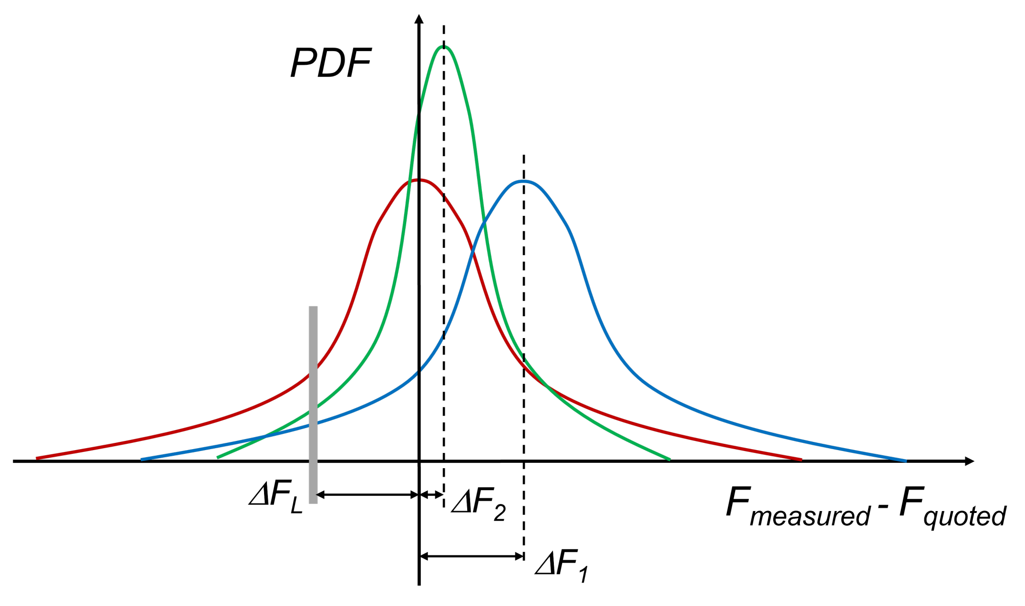
A potential area of application for the machine learning methods discussed in the previous sections is in the quantification and management of uncertainties during the design process. In order to develop a robust design that can deliver good performance across a range of operating conditions, it is necessary to consider the uncertainties affecting the system [50]. Figure 6 illustrates the importance of this for industry, through a probability density function (PDF) that represents the variation between the measured and quoted performance. Examples of performance metrics include the efficiency, life, or operability of a product. The quoted performance, $F_{\mathrm{quoted}}$, is defined as the predicted performance, $F_{\mathrm{predicted}}$, minus a safety margin that includes all uncertainties, $F_{\mathrm{quoted}}=F_{\mathrm{predicted}}-\Delta F_1$. The safety margin is introduced to avoid falling below contractually accepted limits, $\Delta F_L$ (for example 4% on power). The tail of the PDF left of the vertical grey line indicates cases in which a unit does not meet the performance acceptance limit. The red curve assumes $\Delta F_1=0$ and the risk of not meeting the quoted performance is large. The blue curve sets $\Delta F_1>0$ to reduce such risk. In other words, the average expected performance is penalized by shifting the red curve to the right. The amount of shift is directly proportional to the overall uncertainty. The more truncated tails of the green curve show the case in which uncertainty is reduced, or controlled, and the performance prediction is more accurate. The probability mass to the left of the grey line is identical for both the blue and green curves, i.e., both distributions have the same risk of not meeting contractual performance; however, the safety margin of the green curve is smaller ($\Delta F_2<\Delta F_1$) and therefore it is possible to quote a higher performance with the same risk.

The uncertainties affecting a product are typically divided into two categories: aleatoric and epistemic. Aleatoric uncertainties refer to uncertainties arising from random fluctuations in the environment. In the context of turbomachinery, these might arise from: uncertain operating conditions [51]; variations or imperfections introduced in the geometry during manufacturing or caused by wear [52]; and noise present in experimental measurements [53] (constraints $\left(b\right)$, $\left(c\right)$, and $\left(e\right)$ in Figure 2). On the other hand, epistemic uncertainties refer to uncertainties introduced by the simplifications necessary to model a real world system. In addition to numerical effects introduced by truncation, uncertainties introduced by applying theoretical assumptions, a lack of available data, or constraints to a turbulence model come under this category (point $\left(d\right)$ in Figure 2). While aleatoric uncertainties are irreducible, in principle, epistemic uncertainties are reducible and could be minimised, for instance by collecting more data or developing models that more accurately capture the physics.

5.1. Quantifying Aleatoric Uncertainty

The goal of Uncertainty Quantification (UQ) is to estimate the impact of uncertainties on the performance of a product, which might be expressed as a probability distribution or a confidence interval for a given Quantity of Interest (QoI). We first consider the forward propagation of aleatoric uncertainties, in which a joint density over the uncertain parameters affecting the system, $\mathit{\xi }$, is available. At a minimum, the designer is concerned with estimating the first two statistical moments of a QoI, i.e., the mean and standard deviation performance of a design operating in uncertain conditions [54]. Reliability analysis, in which the relatively low probability of the uncertain conditions leading to failure is estimated, is something of an exception to this as this probability will be determined by the distribution tails [55,56]. Nevertheless, the example of estimating the mean and standard deviation of a QoI is instructive, as it illustrates the need for accurate meta-models of expensive CFD simulations for UQ in an industrial setting.

Evaluating the first two statistical moments of an uncertain QoI entails solving the integral for the mean:

$$\mathbb{E}(w)=\int w(\mathit{\xi })f(\mathit{\xi })d\mathit{\xi },$$

(4)

and for the variance:

$$\mathrm{Var}(w)=\int {(w\left(\mathit{\xi }\right)-\mathbb{E}(w))}^{2}f(\mathit{\xi })d\mathit{\xi },$$

(5)

where w represents the QoI and $\mathit{\xi }\in {\Re }^{n_u}$ the uncertain parameters with joint density $f\left(\mathit{\xi }\right)$. These integrals are unlikely to admit an analytical solution. Numerical methods such as stochastic collocation may be employed for low-dimensional uncertain spaces [57]; however, these become computationally intractable for large scale problems. In such cases, Monte Carlo sampling is a popular strategy for approximating these integrals and is particularly effective if the computational model $w\left(\mathit{\xi }\right)$ is cheap to evaluate. An accurate assessment of the aleatoric uncertainties affecting a product requires the evaluation of n Monte Carlo samples, perhaps on the order of n ≈ ${10}^5$–${10}^6$, with the confidence of the estimate of the mean converging as $n^{-\frac{1}{2}}$ [58]. Given the computational costs associated with a single CFD simulation, the statistical assessment of a design using direct Monte Carlo sampling is impractical; a surrogate model or meta-model of the system is required. This meta-model is trained using a limited dataset of CFD simulations, after which the meta-model may be evaluated at what is assumed to be negligible cost. Methods such as non-intrusive Polynomial Chaos Expansions (niPCEs), while effective for low-dimensional uncertain spaces [59], suffer from the curse of dimensionality, where the minimum number of simulations required to determine the coefficients of the expansion grows rapidly with $n_u$. While there is current research targeted at mitigating this aspect of niPCEs (see, e.g., [60,61]), at present, niPCEs are generally infeasible for the high-dimensional problems faced by industry. On the other hand, intrusive Polynomial Chaos Expansions, which require alterations to the CFD code, are criticised for being difficult to implement in an industrial context, although again academics working to mitigate this critique (see, e.g., [62,63]). Addressing these issues presents an opportunity to employ machine learning methods, which have been demonstrated to scale well to high-dimensional spaces, as meta-models that can be used to accelerate simulations, allowing for the accurate statistical assessment of the uncertainties affecting a product.

5.2. Quantifying Epistemic Uncertainty

Quantifying the effects of epistemic uncertainty can be difficult [64]. However, quantifying the structural uncertainties in RANS is a key challenge for industrial CFD simulations as the constraints introduced by theory or experience on a turbulence model are largely responsible for mismatches between simulations and experiments [5,6]. There are already works in the literature that have addressed the issue of model form uncertainty in RANS simulations, which we group into three strategies: perturbation-based; Bayesian-based; or discrepancy modelling.

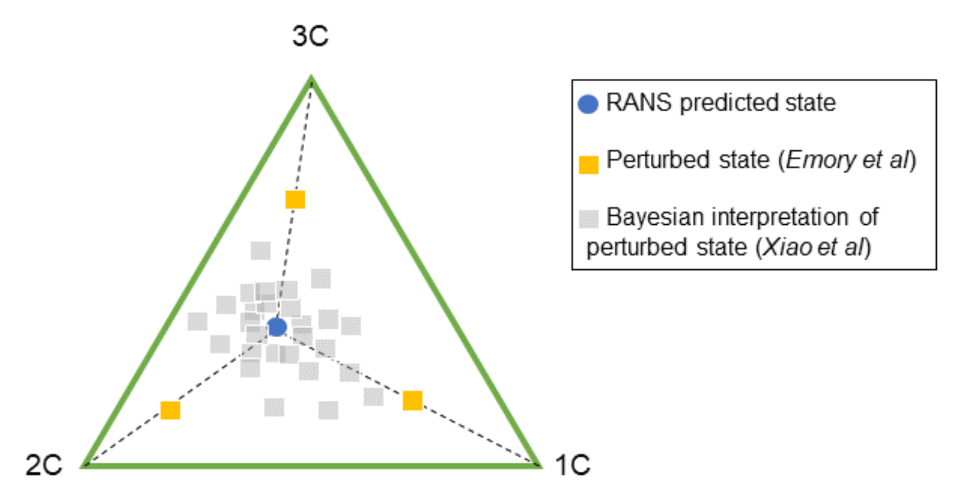
Banerjee et al. [65] demonstrated that the three limiting states of the turbulent anisotropy could be represented as a barycentric map. As an example of the first set of approaches, Gorlé et al. [66] and Emory et al. [67] proposed a perturbation based method for quantifying the epistemic uncertainty in RANS turbulent closures. Uniform eigenvalues perturbations were made to the Reynolds stress anisotropy tensor in the direction of the limiting states of turbulence (1, 2, and 3 component turbulence) to produce a conservative upper bound to the upper bound. These perturbations, and the barycentric coordinate system, are illustrated in Figure 7. Later versions of this method incorporated machine learning, employing a random regression forest to vary the size of the eigenvalue perturbation locally according to the feature importance of a set of 12 dimensionless features [68]. An advantage of the perturbation based approach is that UQ can be performed without requiring a high-fidelity dataset to compare the RANS simulations against, as is the case for the other two categories of approaches.

Bayesian frameworks have been proposed that treat the parameters of the Reynolds stress tensor as a set of uncertain parameters [69,70,71]. Beginning from a set of prior distributions and a joint PDF for the likelihood, posterior probability distributions for these parameters are inferred through a calibration process, in which the predictions of the RANS model are compared against a dataset of high-fidelity observations [72,73]. Figure 7 illustrates this change in perspective using the barycentric coordinate system referenced above. The workflow for the Kalman inversion scheme in Xiao et al. [72] is represented schematically in Figure 8. Rather than perturbing the RANS predicted state towards each of the three limiting cases, in the Bayesian interpretation of the problem, new, physically realisable states are sampled from a posterior distribution. As has been mentioned, a pre-requisite for these Bayesian based methods is that a set of high-fidelity data is available to compare the RANS simulations against. This could be the results of experiments [74,75] or from DNS data.

Finally, there are those methods that develop a statistical model for the discrepancy between RANS and high-fidelity data. In the work of Dow and Wang, for instance, the discrepancy between the turbulent viscosity field predicted by RANS and the field inferred from the DNS data via inverse RANS is modelled as a Gaussian random field [77]. Similarly, the work of Duraisamy et al. [78,79,80] uses field inversion and machine learning methods to develop a functional form of the discrepancies in the model. For further discussion on the topic of quantifying the model form uncertainty in RANS models, we refer the reader to the excellent reviews of Duraisamy et al. [81] and Xiao and Cinella [82]. Section 3 of this paper details recent developments in using machine learning to improve RANS simulations by leveraging high-fidelity data from LES. Often, this is achieved by using machine learning to estimate a set of invariant quantities that can be combined linearly to form the anisotropy tensor in the turbulent closure. The majority of these methods do not consider the uncertainty introduced by this mapping, although some progress has been made in this regard. Geneva and Zabaras [83] introduced a Bayesian formulation of the neural network used by Ling et al. [27] to compute the anisotropy tensor. Through Monte Carlo sampling of a Bayesian Neural Network, they were able to quantify the uncertainty in this term and consequently place probabilistic bounds on the estimated pressure and velocity fields.

5.3. Quantifying Mixed Uncertainty and Visualisation

The methods that have been described so far in this section target the quantification of aleatoric and epistemic (specifically model form) uncertainty separately. Ultimately, tools will need to be developed for industries capable of processing both types of uncertainties simultaneously. This is a challenging problem. However, some progress has been made in this direction within the turbomachinery space [84]. Quantifying the effects of mixed uncertainty may require engineers to reconsider how uncertainty is visualised and communicated. Rather than specifying a single probability distribution for the QoI, a p-box approach that can be used to bound families of likely Cumulative Distribution Functions (CDFs) might be more effective [85,86]. A disadvantage of these methods is that p-boxes are an abstract concept, the meaning of which is difficult to convey to non-experts. Ling and Townsend [87] proposed a classification based approach, using ML classifiers such as Support Vector Machines, to identify the regions of the greatest uncertainty in RANS simulations of flows over several geometries. An advantage of this method is that the levels of uncertainty present in a simulation may be presented intuitively, as can be seen in Figure 9. In risk-averse industries such as aeronautics, new products are heavily scrutinised by regulators before they can be certified [88]. As part of the process of certification, it is necessary to justify the design decisions with the evidence that was available to the designers at the time. For machine learning methods to become incorporated within the design process, it will be essential for the uncertainty present in these methods to be clearly indicated, particularly the predictive uncertainty that can account for epistemic uncertainties arising from a lack of data. At present, the majority of machine learning methods provide point estimations with no way of quantifying the uncertainty in the estimate. As is discussed in the reviews of Hüllermeier and Waegeman [89] and Psaros et al. [90], moving away from ‘black-box’ models and accounting for aleatoric and epistemic uncertainty will be crucial for the massive industrial application of machine learning. The papers review methods that currently accomplish this, such as Bayesian Neural Networks.

5.4. Multi-Fidelity Methods

Finally, industry usually has a wealth of heterogeneous data from the manufacturing, assembly, operation, and servicing of components. These data will be affected by uncertainty to various extents (see, e.g., [91]). It would be beneficial if these data could be used to inform future designs, particularly at the conceptual design phase where the resources available to evaluate candidate designs are limited, but where the decisions taken have a significant impact on the final product [92,93]. Exploiting these data are the motivating philosophy behind the digital twin approach to design, in which sustainable practices throughout the lifecycle of a product are encouraged [94]. However, using a large heterogeneous dataset of historic data is a challenging task due to both the size of the datasets involved and the varying levels of epistemic uncertainty associated with the collection of the data. This is especially true if uncertainty must be propagated between computational models at multiple scales or levels [95]. There is currently a great deal of research within the UQ community directed at multi-fidelity methods, in which generative models that are informed by heterogeneous datasets are developed. Approaches based on Gaussian processes (co-kriging) [96,97], multi-fidelity Polynomial Chaos Expansions [98,99], multi-level Monte Carlo [100], and different forms of physics informed neural networks such as those by Wang and Zhang [101] and Yang et al. [102] have all been proposed for the solution of the PDEs that govern fluid flows. More recently, Pepper et al. [103] presented a Knowledge-Based Neural Network (KBaNN) capable of computing additive corrections to the output of a model based on a coarse computational mesh. The KBaNN was able to generalise to flows that share similar physics. In principle, this approach can be used to add more advanced modelling features and make it possible to develop a bi-fidelity method that leverages data from any existing simulation database.

Of these methods, co-kriging has proved to be particularly popular due to the natural way in which the heterogeneous uncertainties may be handled. An additional advantage is that the predictive uncertainty may be expressed through the kriging variance (see, e.g., [104,105,106,107] for examples in the aeronautics and turbomachinery spaces). In recent years, there has also been emphasis placed on developing ML methods for multi-scale [108,109,110] or multi-level [111,112] uncertainty propagation. However, many of these papers aim at improving low-fidelity model evaluations with datasets from high-fidelity model evaluations, rather than experimental data which is likely to be noisier and more difficult to reconcile due to unresolved physics in the computational models. One approach might be to focus on identifying the “worst offenders” in the low-fidelity model to target. For instance, Lengani et al. used Proper Orthogonal Decomposition (POD) to construct a reduced-order model of a turbine wake in which the modes that contributed the most to unsteady losses could be identified [113]. Nevertheless, for a more comprehensive improvement in the accuracy of simulations, it may be necessary to consider more drastic machine learning approaches. This new paradigm of machine learning methods might offer a means to reconcile simulations of a complex flow field with the available experimental data while simultaneously satisfying the remaining constraints in Figure 2. These new forms of machine learning are discussed in more detail in the following section.

6. New Forms of Machine Learnt Tools

The overwhelming complexity of turbulent flows requires a technology step change to overcome the inherent limits of the approaches followed to date. The so-called turbulence models required by the (U)RANS approach do not attempt to model turbulence; instead, they model the effect of turbulence on a Reynolds-averaged flow field. Such models proved reasonably accurate for engineering applications [5,114], but they have difficulties predicting axial compressor operability [115], heat transfer, aeromechanics, and more generally any off-design operation of aerodynamic bodies [5]. Therefore, the seamless application of (U)RANS is model accuracy limited. The obvious cure is to switch from modelling to resolving the high frequency broad spectrum turbulent motion by LES or DNS. Regretfully, the associated computational cost of realistic scale-resolving simulation is excessive, and the practical application of high-fidelity simulations in industry is computational resources limited.

As discussed earlier in this paper, various forms of machine learning have been used to improve turbulence models—first, for example, GEP and ANNs trained on data from scale-resolving simulations. More recently, an evolution of ANNs, known as Physics Informed Neural Networks (PINNs), introduced a step change in the computer simulation of complex flow fields. Karniadakis et al. [116] provided a detailed explanation of the potential offered by PINNs. This may be understood with reference to the practical example schematized in Figure 2, which describes the mixing of cold and hot streams and represents a typical GT hot-gas-path design problem. The flow field, $\left(a\right)$, must obey fundamental conservation principles such as mass, momentum, and enthalpy balances, under a combined set of inlet conditions, $\left(b\right)$, and boundaries, $\left(c\right)$. The combined set of $\left(a\right)$, $\left(b\right)$, $\left(c\right)$ is enough to perform a computer simulation of the flow and the accuracy of their specification is key to the quality of the final result. However, the physics models adopted in the simulation may not necessarily satisfy the constraints dictated by theory and experience, $\left(d\right)$, and may not guarantee a good match with measurements, $\left(e\right)$. In this case, the only option left to a designer is to start a long and tedious set of iterations to determine the impact of the mesh, model assumptions and boundary conditions on the results, in an attempt to match measurements better. Following from [116], Cai et al. [117] illustrate a way to overcome this bottleneck by training a neural network capable of reproducing the flow field of Figure 2 by using all the available sets of information. With reference to the specific fluid dynamics case of Figure 2, a PINN may be trained to

(a)

Obey the basic conservation principles of the time-averaged Navier–Stokes equations (PDE);

(b)

Match inlet operating conditions (IC);

(c)

Match boundary and geometrical conditions (BC);

(d)

Obey the fundamental turbulence constraints for theory (see, for example, turbulence invariants formulated by Lumley [118]), (TC);

(e)

Match measurements obtained from experiments (ME).

The overall training process may be followed with the help of Figure 10 in which a Neural Network is trained to fulfil the constraints that concur in a penalty function $\Sigma$, which measures the quality and maturity of the PINN training process

$$\Sigma ={\pi }_{\mathrm{PDE}}{\Sigma }_{\mathrm{PDE}}+{\pi }_{\mathrm{IC}}{\Sigma }_{\mathrm{IC}}+{\pi }_{\mathrm{BC}}{\Sigma }_{\mathrm{BC}}+{\pi }_{\mathrm{TC}}{\Sigma }_{\mathrm{TC}}+{\pi }_{\mathrm{ME}}{\Sigma }_{\mathrm{ME}}.$$

(6)

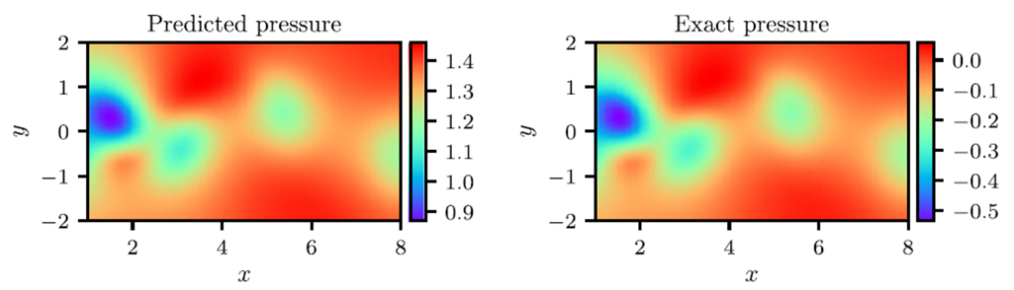
The quantities ${\Sigma }_{\varphi }$ represent the deviation from the expected value (for example, the PDE conservation error), and ${\pi }_{\varphi }$ are a set of weights used to control the severity of the deviation from each separate constraint. The advantage of training a Neural Network based model with this approach is its ability to account for all the information, data, and constraints simultaneously. In fact, the flow field predicted by a PINN trained with this approach will match the measured data $\left(e\right)$ while fulfilling all theoretical constraints and the boundary conditions. The results reported in [116,117] suggest that this is possible, although PINNs and their training process are not ready for massive industrial application. In particular, Cai et al. [117] followed the approach summarized in Equation (6) for the simulation of a portion of the incompressible vortex shedding flow downstream of a cylinder. The set-up of the training dataset had to be appropriately selected, but the results indicated the method was able to capture the most relevant flow features with an $L_2$-norm error ranging from 1% to ≈$10\%$ depending on the velocity component. They further verified their approach on a bow-shock case showing similar accuracy. Eivazi et al. [119] followed a similar approach for the simulation of a boundary layer with adverse, zero, and favourable pressure gradients, confirming that the PINN approach could replicate the boundary layer development with a fair degree of accuracy. The authors also tackled the challenging problem of periodic hills where a sizeable flow separation develops. The predicted flow field, which required inlet conditions, geometry, and boundary values of the static pressure in selected locations, compared well with a reference DNS dataset. In their detailed paper, Raissi et al. [120] described how the solution of well known PDEs, such as the Schrodinger, the Allen-Cahn, and Navier–Stokes equations can be reproduced with PINNs. Their approach differed from that summarized by Equation (6) as they trained the PINN using 200 initial data points randomly sampled from the exact solution available at the initial time step. They used a relatively light network with four hidden layers and 200 neurons per layer to ensure a very good match with the reference exact solution. This is illustrated in Figure 11, highlighting the excellent match between the instantaneous static pressure field downstream of a circular cylinder predicted by the direct solution of the Navier–Stokes equations, and by the PINN.

Although the applications seen to date are relatively simple, they show the huge potential of this method that is not to be seen as a viable replacement for CFD models, but rather as a model capable of incorporating and reconciling multi-fidelity data from different sources, as summarized by Equation (6).

7. Summary and Outlook

Design systems, and particularly turbomachinery design, are increasingly aided by first-principle CFD tools and by general multi-disciplinary optimization methods. This paper summarizes the avenues along which design methods and performance optimization tools can be further improved.

• In a design optimization loop, the quality of a design is measured by interrogating an estimator, in this case, CFD. The quality and robustness of the optimal solution are dictated by the reliability of CFD, the accuracy of which can be boosted by ML.
• Each design iteration, especially when dealing with multidisciplinary verification, is very computationally intensive. ML can improve optimizer convergence by reducing the number of iterations and, more importantly, the cost associated with each design performance analysis.

Along these lines, this paper begins by focusing on the areas in which machine learning is already making a direct impact on CFD within the space of turbomachinery—specifically, where data from higher-fidelity simulations are used to train models which augment lower-fidelity calculations in an attempt to reconcile the model accuracy limiting of (U)RANS with the computational resource limiting of LES or DNS. Machine learning has been successfully used mostly to overcome the difficulties stemming from the modelling of turbulence, the driving mechanism of entropy change. These methods have shown significant promise with improved prediction observed for flows including but not limited to high and low-pressure turbines, cooling flows such as jet in crossflow and turbine internal cooling ducts, waste heat recovery systems, carbon capture and sequestration systems.

Despite their clear potential, it is recognized that at present such methods rarely consider the epistemic uncertainties introduced by these mappings, whilst also assuming single-point specification of initial and boundary conditions. In risk-averse industries such as aviation and marine, as well as power generation for civil and industrial applications where turbomachines are often employed, this uncertainty needs to be quantified and managed to support design decisions and allow certification of products by regulatory bodies. Considering this, current methods are reviewed that account for the uncertainty of some Quantity of Interest in the presence of both aleatoric and epistemic uncertainties. The methods shed light on how UQ can be leveraged to provide some level of assessment of the predictive confidence of these machine learnt models, when applied in previously unseen cases. Improved accuracy will help determine the effect of single components’ performance on the overall engine (i.e., compressor operability, combustion emissions, high-pressure-turbine durability, power turbine efficiency) and eventually aid decisions on the most appropriate corrective action in case of problems. More accurate CFD with a manageable computational effort will also allow the analysis of component to-component interaction, often a cause of unexpected problems (i.e., inlet system and axial compressor instability, combustion chamber and high-pressure turbine durability, power turbine and exhaust system noise, aeroacoustic cavity excitation, to cite a few).

These approaches demonstrate an underutilized but highly important aspect of predictive models if they are to be accepted for large scale integration in an industrial setting. They also bring attention to a fundamental question: how can traditional computational simulation be seamlessly reconciled with the wealth of heterogeneous data often available in industry, each contaminated by varying levels of resolution in space and time, and aleatoric and epistemic uncertainty during their collection. This is by no means a straightforward task. Specification of conservation laws, initial and boundary conditions for some geometry may be sufficient to run a computational simulation but does not guarantee agreement with measured data and design experience.

A recent development that offers the potential to unify these two opposing facets of industrial design comes through the introduction of Physics-Informed Neural Networks (PINNs). PINNs offer a unique opportunity to combine all sources of available information in a single constrained optimisation network. Measured data, data from high-fidelity sources, theoretical physical laws and tried and tested empirical relationships can all be considered simultaneously by incorporating them, with appropriately selected weightings, in the loss function of a learning machine. The development of PINNs brings the field of machine learning in fluid dynamics to a very exciting juncture, where seamless data fusion appears to present itself as a serious contender. Whilst currently in their infancy and applied only to relatively simple applications to date, researchers will inevitably exploit the rich vein that PINNs uncover. This will no doubt come through application to a multitude of more complex problems, to show their pertinence in a general setting and provide novel perspectives to old challenges. Whilst this may be a clear direction, a more thoughtful approach is encouraged at this point, particularly within the industrial setting of turbomachines.

Future data-driven approaches should endeavor to account for the wealth of prior knowledge to reduce the vast high dimensional parameter spaces and reduce the computational complexity of the search for optimal solutions. Predictions using developed models should also be presented with an uncertainty caveat such that practitioners have confidence in the results obtained and can justify the design decisions taken as a result. Although fully replacing current conventional methods will take time, there is already a clear path toward new methods with a wider validity range—those that, with the help of ML, make the best use of measurements from both dedicated scaled-down tests and high-fidelity field data, enforce theory and improve the prediction accuracy of computational tools from early to detailed design.

References

- Gas Turbine World 2020 GTW Handbook; Pequot Publishing Inc.: Fairfield, CT, USA, 2020.
- Sources of Greenhouse Gas Emissions. Available online: https://www.epa.gov/ghgemissions/sources-greenhouse-gas-emissions (accessed on 26 October 2021).
- Michelassi, V.; Ling, J. Challenges and opportunities for artificial intelligence and high-fidelity simulations in turbomachinery applications: A perspective. J. Glob. Power Propuls. Soc. 2021, 1–14. [Google Scholar] [CrossRef]
- Denton, J.D.; Dawes, W.N. Computational fluid dynamics for turbomachinery. J. Mech. Eng. Sci. 1998, 213, 107–124. [Google Scholar] [CrossRef]
- Sandberg, R.D.; Michelassi, V. The current state of high-fidelity simulations for main gas path turbomachinery components and their industrial impact. Flow Turbul. Combust. 2019, 102, 797–848. [Google Scholar] [CrossRef]
- Laskowski, G.; Kopriva, J.; Michelassi, V.; Shankaran, S.; Paliath, U.; Bhaskaran, R.; Wang, Q.; Talnikar, C.; Wang, Z.; Jia, F. Future Directions of High Fidelity CFD for Aerothermal Turbomachinery Analysis and Design. In Proceedings of the 46th AIAA Fluid Dynamics Conference, Washington, DC, USA, 13–17 June 2016; p. 3322. [Google Scholar]
- Akolekar, H.D.; Sandberg, R.D.; Hutchins, N.; Michelassi, V.; Laskowski, G. Machine-Learnt Turbulence Closures for Low-Pressure Turbines with Unsteady Inflow Conditions. J. Turbomach. 2019, 141, 101009. [Google Scholar] [CrossRef]
- Michelassi, V.; Chen, L.; Pichler, R.; Sandberg, R.D.; Bhaskaran, R. High-fidelity simulations of low-pressure turbines: Effect of flow coefficient and reduced frequency on losses. ASME J. Turbomach. 2016, 138, 111006. [Google Scholar] [CrossRef]
- Pichler, R.; Michelassi, V.; Sandberg, R.D.; Ong, J. Highly Resolved LES Study of Gap Size Effect on Low-Pressure Turbine Stage. ASME J. Turbomach. 2017, 140, 021003. [Google Scholar]
- Meloni, R.; Ceccherini, G.; Michelassi, V.; Riccio, G. Analysis of the self-excited dynamics of a heavy-duty annular combustion chamber by large-eddy simulation. J. Eng. Gas Turbines Power 2019, 141, 111016. [Google Scholar] [CrossRef]
- Sandberg, R.D.; Michelassi, V. Fluid Dynamics of Axial Turbomachinery: Blade- and Stage-Level Simulations and Models. Annu. Rev. Fluid Mech. 2022, 54, 255–285. [Google Scholar] [CrossRef]
- Slotnick, J.; Khodadoust, A.; Alonso, J.; Darmofal, D. CFD Vision 2030 Study: A Path to Revolutionary Computational Aerosciences; Technical Report; NASA Langley Research Center: Hampton, VA, USA, 2014. [Google Scholar]
- Jones, W.; Launder, B. The calculation of low-Reynolds-number phenomena with a two-equation model of turbulence. Int. J. Heat Mass Transf. 1973, 16, 1119–1130. [Google Scholar] [CrossRef]
- Lopez, D.I.; Ghisu, T.; Shahpar, S. Global Optimisation of a Transonic Fan Blade Through AI-Enabled Active Subspaces. J. Turbomach. 2021, 14, 011013. [Google Scholar]
- Gaymann, A.; Montomoli, F.; Pietropaoli, M. Robust Fluid Topology Optimization Using Polynomial Chaos Expansions: TOffee. In Turbo Expo: Power for Land, Sea, and Air; Turbomachinery: London, UK, 2018; Volume 2D. [Google Scholar] [CrossRef]
- Gatski, T.; Speziale, C. On explicit algebraic stress models for complex turbulent flows. J. Fluid Mech. 1993, 254, 59–78. [Google Scholar] [CrossRef] [Green Version]
- Zhao, Y.; Akolekar, H.D.; Weatheritt, J.; Michelassi, V.; Sandberg, R.D. RANS turbulence model development using CFD-driven machine learning. J. Comput. Phys. 2020, 411, 109413. [Google Scholar] [CrossRef] [Green Version]
- Wallin, S.; Johansson, A. An explicit algebraic Reynolds stress model for incompressible and compressible turbulent flows. J. Fluid Mech. 2000, 403, 89–132. [Google Scholar] [CrossRef]
- Park, J.; Choi, H. Toward neural-network-based large eddy simulation: Application to turbulent channel flow. J. Fluid Mech. 2021, 914, A16. [Google Scholar] [CrossRef]
- Weatheritt, J.; Sandberg, R.D. Hybrid Reynolds-Averaged/Large-Eddy Simulation Methodology from Symbolic Regression: Formulation and Application. AIAA J. 2017, 55, 3734–3746. [Google Scholar] [CrossRef]
- Weatheritt, J.; Sandberg, R.D. A novel evolutionary algorithm applied to algebraic modifications of the RANS stress-strain relationship. J. Comput. Phys. 2016, 325, 22–37. [Google Scholar] [CrossRef]
- Pope, S.B. A more general effective-viscosity hypothesis. J. Fluid Mech. 1975, 72, 331–340. [Google Scholar] [CrossRef] [Green Version]
- Weatheritt, J.; Pichler, R.; Sandberg, R.D.; Laskowski, G.; Michelassi, V. Machine Learning for Turbulence Model Development Using a High-Fidelity HPT Cascade Simulation. In Proceedings of the Turbomachinery Technical Conference and Exposition, Charlotte, NC, USA, 26–30 June 2017; pp. 1–12. [Google Scholar] [CrossRef]
- Weatheritt, J.; Zhao, Y.; Sandberg, R.D.; Mizukami, S.; Tanimoto, K. Data-driven scalar-flux model development with application to jet in cross flow. Int. J. Heat Mass Transf. 2019, 147, 118931. [Google Scholar] [CrossRef]
- Hammond, J.; Montomoli, F.; Pietropaoli, M.; Sandberg, R.; Michelassi, V. Machine Learning for the Development of Data Driven Turbulence Closures in Coolant Systems. J. Turbomach. 2022, 144, 081003. [Google Scholar] [CrossRef]
- Frey Marioni, Y.; Ortiz, E.A.D.T.; Cassinelli, A.; Montomoli, F.; Adami, P.; Vazquez, R. A machine learning approach to improve turbulence modelling from DNS data using neural networks. Int. J. Turbomach. Propuls. Power 2021, 6, 17. [Google Scholar] [CrossRef]
- Ling, J.; Kurzawski, A.; Templeton, J. Reynolds averaged turbulence modelling using deep neural networks with embedded invariance. J. Fluid Mech. 2016, 807, 155–166. [Google Scholar] [CrossRef]
- Weatheritt, J.; Sandberg, R.D.; Ling, J.; Saez, G.; Bodart, J. A Comparative Study of Contrasting Machine Learning Frameworks Applied to RANS Modeling of Jets in Crossflow. In Proceedings of the ASME Turbo Expo 2017: Turbomachinery Technical Conference and Exposition, Charlotte, NC, USA, 26–30 June 2017. GT2017-63403. [Google Scholar]
- Tucker, P. Computation of unsteady turbomachinery flows: Part1–Progress and Challenges. Prog. Aerosp. Sci. 2011, 47, 522–545. [Google Scholar] [CrossRef]
- Michelassi, V.; Pichler, R.; Chen, L.; Sandberg, R.D. Compressible Direct Numerical Simulation of Low-Pressure Turbines: Part II—Effect of Inflow Disturbances. ASME J. Turbomach. 2015, 137, 071005-1–071005-12. [Google Scholar] [CrossRef]
- Lav, C.; Sandberg, R.D.; Philip, J. A framework to develop data-driven turbulence models for flows with organised unsteadiness. J. Comp. Phys. 2019, 383, 148–165. [Google Scholar] [CrossRef]
- Van de Wall, A.G.; Kadambi, J.R.; Adamczyk, J.J. A transport model for the deterministic stresses associated with turbomachinery blade row interactions. J. Turbomach. 2000, 122, 593–603. [Google Scholar] [CrossRef]
- Hammond, J.; Pietropaoli, M.; Montomoli, F. Topology optimisation of turbulent flow using data-driven modelling. Struct. Multidiscip. Optim. 2022, 65, 49. [Google Scholar] [CrossRef]
- Ali, Z.; Tyacke, J.; Tucker, P.G.; Shahpar, S. Block Topology Generation for Structured Multi-block Meshing with Hierarchical Geometry Handling. Procedia Eng. 2016, 163, 212–224. [Google Scholar] [CrossRef] [Green Version]
- Toosi, S.; Larsson, J. Grid-adaptation and convergence-verification in large eddy simulation: A robust and systematic approach. In Proceedings of the 2018 Fluid Dynamics Conference, Atlanta, GA, USA, 25–29 June 2018; pp. 1–24. [Google Scholar] [CrossRef]
- Rezaeiravesh, S.; Liefvendahl, M. Effect of grid resolution on large eddy simulation of wall-bounded turbulence. Phys. Fluids 2018, 30, 055106. [Google Scholar] [CrossRef] [Green Version]
- Tyacke, J.; Vadlamani, N.R.; Trojak, W.; Watson, R.; Ma, Y.; Tucker, P.G. Turbomachinery simulation challenges and the future. Prog. Aerosp. Sci. 2019, 110, 100554. [Google Scholar] [CrossRef]
- Kochkov, D.; Smith, J.A.; Alieva, A.; Wang, Q.; Brenner, M.P.; Hoyer, S. Machine learning—Accelerated computational fluid dynamics. Proc. Natl. Acad. Sci. USA 2021, 118, e2101784118. [Google Scholar] [CrossRef]
- Gao, H.; Sun, L.; Wang, J.X. Super-resolution and denoising of fluid flow using physics-informed convolutional neural networks without high-resolution labels. Phys. Fluids 2021, 33, 073603. [Google Scholar] [CrossRef]
- Fotiadis, S.; Pignatelli, E.; Valencia, M.L.; Cantwell, C.; Storkey, A.; Bharath, A.A. Comparing Recurrent and Convolutional Neural Networks for Predicting Wave Propagation. arXiv 2020, arXiv:2002.08981. [Google Scholar]
- Sorteberg, W.E.; Garasto, S.; Cantwell, C.C.; Bharath, A.A. Approximating the Solution of Surface Wave Propagation Using Deep Neural Networks. In Proceedings of the 32nd Conference on Neural Information Processing Systems (NeurIPS), Montreal, QC, Canada, 3–8 December 2018; pp. 246–256. [Google Scholar] [CrossRef]
- Wang, Y.; Gao, Z.; Long, M.; Wang, J.; Yu, P.S. PredRNN++: Towards a resolution of the deep-in-time dilemma in spatiotemporal predictive learning. Int. Conf. Mach. Learn. 2018, 11, 8122–8131. [Google Scholar]
- Thuerey, N.; Weissenow, K.; Prantl, L.; Hu, X. Deep learning methods for reynolds-averaged navier–stokes simulations of airfoil flows. AIAA J. 2020, 58, 25–36. [Google Scholar] [CrossRef]
- Dosovitskiy, A.; Fischer, P. FlowNet: Learning Optical Flow with Convolutional Networks. arXiv 2015, arXiv:1504.06852. [Google Scholar]
- De Bézenac, E.; Pajot, A.; Gallinari, P. Deep learning for physical processes: Incorporating prior scientific knowledge. In Proceedings of the 6th International Conference on Learning Representations, ICLR 2018—Conference Track Proceedings, Vancouver, BC, Canada, 30 April–3 May 2018; IOP Publishing: Bristol, UK, 2018. [Google Scholar]
- Vinuesa, R.; Brunton, S.L. The Potential of Machine Learning to Enhance Computational Fluid Dynamics. arXiv 2021, arXiv:2110.02085. [Google Scholar]
- Brunton, S.L.; Noack, B.R.; Koumoutsakos, P. Machine Learning for Fluid Mechanics. Annu. Rev. Fluid Mech. 2020, 52, 477–508. [Google Scholar] [CrossRef] [Green Version]
- Obiols-Sales, O.; Vishnu, A.; Malaya, N.; Chandramowliswharan, A. CFDNet: A deep learning-based accelerator for fluid simulations. In Proceedings of the International Conference on Supercomputing, Barcelona, Spain, 29 June–2 July 2020. [Google Scholar] [CrossRef]
- Leer, M.; Kempf, A. Fast Flow Field Estimation for Various Applications with A Universally Applicable Machine Learning Concept. Flow Turbul. Combust. 2021, 107, 175–200. [Google Scholar] [CrossRef]
- Bertini, F.; Credi, M.; Marconcini, M.; Giovannini, M. A Path Toward the Aerodynamic Robust Design of Low Pressure Turbines. J. Turbomach. 2012, 135, 021018. [Google Scholar] [CrossRef]
- Satish, T.; Murthy, R.; Singh, A. Analysis of uncertainties in measurement of rotor blade tip clearance in gas turbine engine under dynamic condition. Proc. Inst. Mech. Eng. Part G J. Aerosp. Eng. 2014, 228, 652–670. [Google Scholar] [CrossRef]
- Montomoli, F.; Massini, M.; Salvadori, S. Geometrical uncertainty in turbomachinery: Tip gap and fillet radius. Comput. Fluids 2011, 46, 362–368. [Google Scholar] [CrossRef]
- Notaristefano, A.; Gaetani, P.; Dossena, V.; Fusetti, A. Uncertainty Evaluation on Multi-Hole Aerodynamic Pressure Probes. J. Turbomach. 2021, 143, 091001. [Google Scholar] [CrossRef]
- Montomoli, F.; Carnevale, M.; Massini, M.; D’Ammaro, A.; Salvadori, S. Uncertainty Quantification in Computational Fluid Dynamics and Aircraft Engines; Springer: London, UK, 2015. [Google Scholar]
- Sepe, M.; Graziano, A.; Badora, M.; Di Stazio, A.; Bellani, L.; Compare, M.; Zio, E. A physics-informed machine learning framework for predictive maintenance applied to turbomachinery assets. J. Glob. Power Propuls. Soc. 2021, 1–15. [Google Scholar] [CrossRef]
- Gottschalk, H.; Saadi, M.; Doganay, O.T.; Klamroth, K.; Schmitz, S. Adjoint Method to Calculate the Shape Gradients of Failure Probabilities for Turbomachinery Components. In Turbo Expo: Power for Land, Sea, and Air; Turbomachinery: London, UK, 2018; Volume 7A. [Google Scholar] [CrossRef]
- Eldred, M.; Burkardt, J. Comparison of Non-Intrusive Polynomial Chaos and Stochastic Collocation Methods for Uncertainty Quantification. In Proceedings of the 47th AIAA Aerospace Sciences Meeting Including the New Horizons Forum and Aerospace Exposition, Orlando, FL, USA, 5–8 January 2009. [Google Scholar] [CrossRef] [Green Version]
- Hanson, J.; Beard, B. Applying Monte Carlo Simulation to Launch Vehicle Design and Requirements Verification. In Proceedings of the AIAA Guidance, Navigation, and Control Conference, Toronto, ON, Canada, 2–5 August 2010. [Google Scholar]
- Knio, O.M.; Maître, O.P.L. Uncertainty propagation in CFD using polynomial chaos decomposition. Fluid Dyn. Res. 2006, 38, 616–640. [Google Scholar] [CrossRef]
- Zhou, Y.; Lu, Z.; Hu, J.; Hu, Y. Surrogate modeling of high-dimensional problems via data-driven polynomial chaos expansions and sparse partial least square. Comput. Methods Appl. Mech. Eng. 2020, 364, 112906. [Google Scholar] [CrossRef]
- Salis, C.; Zygiridis, T. Dimensionality Reduction of the Polynomial Chaos Technique Based on the Method of Moments. IEEE Antennas Wirel. Propag. Lett. 2018, 17, 2349–2353. [Google Scholar] [CrossRef]
- Papageorgiou, A.K.; Papoutsis-Kiachagias, E.M.; Giannakoglou, K.C. Development and assessment of an intrusive polynomial chaos expansion-based continuous adjoint method for shape optimization under uncertainties. Int. J. Numer. Methods Fluids 2022, 94, 59–75. [Google Scholar] [CrossRef]
- Chatzimanolakis, M.; Kantarakias, K.D.; Asouti, V.; Giannakoglou, K. A painless intrusive polynomial chaos method with RANS-based applications. Comput. Methods Appl. Mech. Eng. 2019, 348, 207–221. [Google Scholar] [CrossRef]
- Uusitalo, L.; Lehikoinen, A.; Helle, I.; Myrberg, K. An overview of methods to evaluate uncertainty of deterministic models in decision support. Environ. Model. Softw. 2015, 63, 24–31. [Google Scholar] [CrossRef] [Green Version]
- Banerjee, S.; Krahl, R.; Durst, F.; Zenger, C. Presentation of anisotropy properties of turbulence, invariants versus eigenvalue approaches. J. Turbul. 2007, 8, N32. [Google Scholar] [CrossRef]
- Gorlé, C.; Emory, M.; Larsson, J.; Iaccarino, G. Epistemic Uncertainty Quantification for RANS Modeling of the Flow over a Wavy Wall; Annual Research Briefs; Center for Turbulence Research: Stanford, CA, USA, 2012; pp. 81–91. [Google Scholar]
- Emory, M.; Larsson, J.; Iaccarino, G. Modeling of structural uncertainties in Reynolds-averaged Navier–Stokes closures. Phys. Fluids 2013, 25, 110822. [Google Scholar] [CrossRef]
- Heyse, J.F.; Mishra, A.A.; Iaccarino, G. Estimating RANS model uncertainty using machine learning. J. Glob. Power Propuls. Soc. 2021, 1–14. [Google Scholar] [CrossRef]
- Cheung, S.H.; Oliver, T.A.; Prudencio, E.E.; Prudhomme, S.; Moser, R.D. Bayesian uncertainty analysis with applications to turbulence modeling. Reliab. Eng. Syst. Saf. 2011, 96, 1137–1149. [Google Scholar] [CrossRef]
- Oliver, T.A.; Moser, R.D. Bayesian uncertainty quantification applied to RANS turbulence models. J. Phys. Conf. Ser. 2011, 318, 042032. [Google Scholar] [CrossRef] [Green Version]
- Oliver, T.; Moser, R. Uncertainty Quantification for RANS Turbulence Model Predictions. In APS Division of Fluid Dynamics Meeting Abstracts; American Physical Society: College Park, MD, USA, 2009; Available online: http://meetings.aps.org/link/BAPS.2009.DFD.LC.4 (accessed on 2 February 2022).
- Xiao, H.; Wu, J.L.; Wang, J.X.; Sun, R.; Roy, C. Quantifying and reducing model-form uncertainties in Reynolds-averaged Navier–Stokes simulations: A data-driven, physics-informed Bayesian approach. J. Comput. Phys. 2016, 324, 115–136. [Google Scholar] [CrossRef] [Green Version]
- Edeling, W.N.; Cinnella, P.; Dwight, R.P.; Bijl, H. Bayesian estimates of parameter variability in the k-ϵ turbulence model. J. Comput. Phys. 2014, 258, 73–94. [Google Scholar] [CrossRef] [Green Version]
- Edeling, W.; Cinnella, P.; Dwight, R.P. Predictive RANS simulations via Bayesian model-scenario averaging. J. Comp. Phys. 2014, 275, 65–91. [Google Scholar] [CrossRef] [Green Version]
- Li, J.P.; Zeng, F.Z.; Chen, S.S.; Zhang, K.L.; Yan, C. Bayesian model evaluation of three k–ω turbulence models for hypersonic shock wave–boundary layer interaction flows. Acta Astronaut. 2021, 189, 143–157. [Google Scholar] [CrossRef]
- Xiao, H.; Wang, J.X.; Ghanem, R.G. A random matrix approach for quantifying model-form uncertainties in turbulence modeling. Comput. Methods Appl. Mech. Eng. 2017, 313, 941–965. [Google Scholar] [CrossRef] [Green Version]
- Dow, E.; Wang, Q. Quantification of structural uncertainties in the k-ω turbulence model. In Proceedings of the AIAA/ASME/ASCE/AHS/ASC Structures, Structural Dynamics and Materials Conference, Denver, CO, USA, 4–7 April 2011. [Google Scholar] [CrossRef] [Green Version]
- Tracey, B.D.; Duraisamy, K.; Alonso, J.J. A machine learning strategy to assist turbulence model development. In Proceedings of the 53rd AIAA Aerospace Sciences Meeting, Kissimmee, FL, USA, 5–9 January 2015; p. 1287. [Google Scholar]
- Parish, E.J.; Duraisamy, K. A paradigm for data-driven predictive modeling using field inversion and machine learning. J. Comput. Phys. 2016, 305, 758–774. [Google Scholar] [CrossRef] [Green Version]
- Singh, A.P.; Duraisamy, K. Using field inversion to quantify functional errors in turbulence closures. Phys. Fluids 2016, 28, 045110. [Google Scholar] [CrossRef]
- Duraisamy, K.; Iaccarino, G.; Xiao, H. Turbulence Modeling in the Age of Data. Ann. Rev. Fluid Mech. 2019, 51, 357–377. [Google Scholar] [CrossRef] [Green Version]
- Xiao, H.; Cinnella, P. Quantification of model uncertainty in RANS simulations: A review. Prog. Aerosp. Sci. 2019, 108, 1–31. [Google Scholar] [CrossRef] [Green Version]
- Geneva, N.; Zabaras, N. Quantifying model form uncertainty in Reynolds-averaged turbulence models with Bayesian deep neural networks. J. Comput. Phys. 2019, 383, 125–147. [Google Scholar] [CrossRef] [Green Version]
- McKeand, A.M.; Gorguluarslan, R.M.; Choi, S.K. Stochastic analysis and validation under aleatory and epistemic uncertainties. Reliab. Eng. Syst. Saf. 2021, 205, 107258. [Google Scholar] [CrossRef]
- Pepper, N.; Montomoli, F.; Sharma, S. Data fusion for Uncertainty Quantification with Non-Intrusive Polynomial Chaos. Comput. Methods Appl. Mech. Eng. 2021, 374, 113577. [Google Scholar] [CrossRef]
- He, Q. Model validation based on probability boxes under mixed uncertainties. Adv. Mech. Eng. 2019, 11, 1687814019847411. [Google Scholar] [CrossRef]
- Ling, J.; Templeton, J. Evaluation of machine learning algorithms for prediction of regions of high Reynolds averaged Navier Stokes uncertainty. Phys. Fluids 2015, 27, 085103. [Google Scholar] [CrossRef]
- Freeman, R. 1—New welding techniques for aerospace materials. In Welding and Joining of Aerospace Materials, 2nd ed.; Woodhead Publishing Series in Welding and Other Joining Technologies; Chaturvedi, M., Ed.; Woodhead Publishing: Cambridge, UK, 2021; pp. 1–19. [Google Scholar] [CrossRef]
- Hüllermeier, E.; Waegeman, W. Aleatoric and epistemic uncertainty in machine learning: An introduction to concepts and methods. Mach. Learn. 2021, 110, 457–506. [Google Scholar] [CrossRef]
- Psaros, A.F.; Meng, X.; Zou, Z.; Guo, L.; Karniadakis, G.E. Uncertainty Quantification in Scientific Machine Learning: Methods, Metrics, and Comparisons. arXiv 2022, arXiv:2201.07766. [Google Scholar]
- McCroskey, W. A critical Assessment of Wind Tunnel Results for the NACA 0012 Airfoil; Technical Report; National Aeronautics and Space Administration: Moffett Field, CA, USA, 1987. [Google Scholar]
- Mavris, D.; DeLaurentis, D. Methodology for Examining the Simultaneous Impact of Requirements, Vehicle Characteristics, and Technologies on Military Aircraft Design. ICAS 2000, 144, 1–12. [Google Scholar]
- Saravi, M.; Newnes, L.; Mileham, A.; Goh, Y. Estimating Cost at the Conceptual Design Stage to Optimize Design in terms of Performance and Cost. In Collaborative Product and Service Life Cycle Management for a Sustainable World; Advanced Concurrent Engineering; Curran, R., Chou, S., Trappey, A., Eds.; Springer: Berlin, Germany, 2008. [Google Scholar]
- Xie, R.; Chen, M.; Liu, W.; Jian, H.; Shi, Y. Technologies for Turbomachinery in a Life Cycle Perspective: A Review. Sustainability 2021, 13, 2495. [Google Scholar] [CrossRef]
- Babuška, I.; Nobile, F.; Tempone, R. Reliability of computational science. Numer. Methods Partial. Differ. Equ. 2007, 23, 753–784. [Google Scholar] [CrossRef] [Green Version]
- Kennedy, M.C.; O’Hagan, A. Bayesian calibration of computer models. J. R. Stat. Soc. Ser. B (Stat. Methodol.) 2001, 63, 425–464. [Google Scholar] [CrossRef]
- Forrester, A.I.; Sóbester, A.; Keane, A.J. Multi-fidelity optimization via surrogate modelling. Proc. R. Soc. A Math. Phys. Eng. Sci. 2007, 463, 3251–3269. [Google Scholar] [CrossRef]
- Eldred, M.S.; Ng, L.W.T.; Barone, M.F.; Domino, S.P. Multifidelity Uncertainty Quantification Using Spectral Stochastic Discrepancy Models. In Handbook of Uncertainty Quantification; Ghanem, R., Higdon, D., Owhadi, H., Eds.; Springer International Publishing: Cham, Switzerland, 2015; pp. 991–1040. [Google Scholar]
- Yan, L.; Zhou, T. Adaptive multi-fidelity polynomial chaos approach to Bayesian inference in inverse problems. J. Comput. Phys. 2019, 381, 110–128. [Google Scholar] [CrossRef] [Green Version]
- Giles, M.B. Multilevel Monte Carlo methods. Acta Numer. 2015, 24, 259–328. [Google Scholar] [CrossRef] [Green Version]
- Wang, F.; Zhang, Q.J. Knowledge-based neural models for microwave design. IEEE Trans. Microw. Theory Tech. 1997, 45, 2333–2343. [Google Scholar] [CrossRef]
- Yang, L.; Meng, X.; Karniadakis, G.E. B-PINNs: Bayesian physics-informed neural networks for forward and inverse PDE problems with noisy data. J. Comput. Phys. 2021, 425, 109913. [Google Scholar] [CrossRef]
- Pepper, N.; Gaymann, A.; Sharma, S.; Montomoli, F. Local bi-fidelity field approximation with Knowledge Based Neural Networks for Computational Fluid Dynamics. Sci. Rep. 2021, 11, 14459. [Google Scholar] [CrossRef]
- Laurenceau, J.; Sagaut, P. Building efficient response surfaces of aerodynamic functions with kriging and cokriging. AIAA J. 2008, 46, 498–507. [Google Scholar] [CrossRef] [Green Version]
- Wang, Q.; Song, L.; Guo, Z.; Li, J. Transfer Optimization in Accelerating the Design of Turbomachinery Cascades. In Turbo Expo: Power for Land, Sea, and Air; Turbomachinery: London, UK, 2020; Volume 2D. [Google Scholar] [CrossRef]
- Han, Z.H.; Zimmermann, R.; Goretz, S. A New Cokriging Method for Variable-Fidelity Surrogate Modeling of Aerodynamic Data. In Proceedings of the 48th AIAA Aerospace Sciences Meeting Including the New Horizons Forum and Aerospace Exposition, Orlando, FL, USA, 4–7 January 2010. [Google Scholar] [CrossRef] [Green Version]
- Rumpfkeil, M.; Yamazaki, W.; Dimitri, M. A Dynamic Sampling Method for Kriging and Cokriging Surrogate Models. In Proceedings of the 49th AIAA Aerospace Sciences Meeting including the New Horizons Forum and Aerospace Exposition, Orlando, FL, USA, 4–7 January 2011. [Google Scholar] [CrossRef] [Green Version]
- Chan, S.; Elsheikh, A.H. A machine learning approach for efficient uncertainty quantification using multiscale methods. J. Comput. Phys. 2018, 354, 493–511. [Google Scholar] [CrossRef] [Green Version]
- Peng, G.C.; Alber, M.; Tepole, A.B.; Cannon, W.R.; De, S.; Dura-Bernal, S.; Garikipati, K.; Karniadakis, G.; Lytton, W.W.; Perdikaris, P.; et al. Multiscale modeling meets machine learning: What can we learn? Arch. Comput. Methods Eng. 2021, 28, 1017–1037. [Google Scholar] [CrossRef] [PubMed] [Green Version]
- Trehan, S.; Durlofsky, L. Machine-learning-based modeling of coarse-scale error, with application to uncertainty quantification. Comput. Geosci. 2018, 22, 1093–1113. [Google Scholar] [CrossRef]
- Lye, K.O.; Mishra, S.; Molinaro, R. A multi-level procedure for enhancing accuracy of machine learning algorithms. Eur. J. Appl. Math. 2021, 32, 436–469. [Google Scholar] [CrossRef]
- Jabarullah Khan, N.K.; Elsheikh, A.H. A machine learning based hybrid multi-fidelity multi-level Monte Carlo method for uncertainty quantification. Front. Environ. Sci. 2019, 7, 105. [Google Scholar] [CrossRef] [Green Version]
- Lengani, D.; Simoni, D.; Pichler, R.; Sandberg, R.D.; Michelassi, V.; Bertini, F. On the Identification and Decomposition of the Unsteady Losses in a Turbine Cascade. J. Turbomach. 2019, 141, 031005. [Google Scholar] [CrossRef]
- Denton, J. The 1993 IGTI Scholar Lecture: Loss Mechanics in Turbomachines. ASME J. Turbomach. 1993, 115, 621–656. [Google Scholar] [CrossRef]
- Leggett, J.; Priebe, S.; Shabbir, A.; Michelassi, V.; Sandberg, R.; Richardson, E. LES Loss Prediction in an Axial Compressor Cascade at Off-Design Incidences with Free Stream Disturbances. ASME J. Turbomach. 2018, 7, 071005. [Google Scholar] [CrossRef] [Green Version]
- Karniadakis, G.E.; Kevrekidis, I.G.; Lu, L.; Perdikaris, P.; Wang, S.; Yang, L. Physics-informed machine learning. Nat. Rev. Phys. 2021, 3, 422–440. [Google Scholar] [CrossRef]
- Cai, S.; Mao, Z.; Wang, Z.; Yin, M.; Karniadakis, G.E. Physics-informed neural networks (PINNs) for fluid mechanics: A review. arXiv 2021, arXiv:2105.09506. [Google Scholar] [CrossRef]
- Lumley, J. Toward a turbulent constitutive relation. J. Fluid Mech. 1970, 41, 413–434. [Google Scholar] [CrossRef]
- Eivazi, H.; Tahani, M.; Schlatter, P.; Vinuesa, R. Physics-informed neural networks for solving Reynolds-averaged Navier–Stokes equations. arXiv 2021, arXiv:2107.10711. [Google Scholar]
- Raissi, M.; Perdikaris, P.; Karniadakis, G. Physics-informed neural networks: A deep learning framework for solving forward and inverse problems involving nonlinear partial differential equations. J. Comput. Phys. 2019, 378, 686–707. [Google Scholar] [CrossRef]
Figure 1.
Comparison of the different approaches for modelling turbulence: (a) Computational expense against accuracy for each approach; (b) the correlation of each method to the energy spectrum, highlighting which portion of the spectrum is resolved or modelled in each case.
Figure 2.
Data and constraints contributing to the definition of the flow field. The picture illustrates a snapshot of the mixing of cold and hot streams.
Figure 3.
Energy spectrum for turbomachinery showing the different scales at which deterministic frequencies can contaminate the canonical spectrum.
Figure 4.
Schematic of the branches by which higher-fidelity scale-resolving simulations can be used as datasets to inform the development of lower-order models.
Figure 5.
Training verification strategies which can broadly be split into two main categories: frozen training and RANS-in-the-loop.
Figure 6.
Effect of uncertainty on quoted performance. The red line corresponds to an uncertain parameter with no saftety margin and high probability of failing performance standards. The blue line shows the same uncertain parameter with a large saftey margin required to reduce failure probability to an acceptable level. The green line shows how the safety margin achieving same failure probability can be reduced by reducing the overall uncertainty.
Figure 7.
Barycentric map of the physically realisable states of turbulence as a combination of three limiting states of turbulence: one, two, and three components (1C, 2C, and 3C, respectively) and represented the perspectives for pertubation based and Bayesian based methods of UQ in this space. Adapted from [67,76]. Copyright 2016 Elsevier B.V.
Figure 8.
A schematic illustrating the Kalman inverison scheme: the posterior distribution for the uncertain parameters in RANS is adjusted to reconcile the ensemble of propagated states as closely as possible with the observations. Adapted from [72]. Copyright 2016 Elsevier Inc.
Figure 9.
Perspectives for visualising the results of uncertainty analyses: illustration of a p-box (top) and representation of RANS uncertainty from Ling and Townsend (bottom, adapted from [87]. Copyright 2015 AIP Publishing LLC.).
Figure 10.
A generalized schematic of the Physics Informed Neural Network (PINN) approach.
Figure 11.
Instantaneous static pressure in the vortex shedding region downstream of circular cylinder. Reproduced with permission from [120]. Copyright 2018 Elsevier Inc.
Publisher’s Note: MDPI stays neutral with regard to jurisdictional claims in published maps and institutional affiliations. |
© 2022 by the authors. Licensee MDPI, Basel, Switzerland. This article is an open access article distributed under the terms and conditions of the Creative Commons Attribution (CC BY-NC-ND) license (https://creativecommons.org/licenses/by-nc-nd/4.0/).
Share and Cite
MDPI and ACS Style
Hammond, J.; Pepper, N.; Montomoli, F.; Michelassi, V. Machine Learning Methods in CFD for Turbomachinery: A Review. Int. J. Turbomach. Propuls. Power 2022, 7, 16. https://doi.org/10.3390/ijtpp7020016
AMA Style
Hammond J, Pepper N, Montomoli F, Michelassi V. Machine Learning Methods in CFD for Turbomachinery: A Review. International Journal of Turbomachinery, Propulsion and Power. 2022; 7(2):16. https://doi.org/10.3390/ijtpp7020016
Chicago/Turabian StyleHammond, James, Nick Pepper, Francesco Montomoli, and Vittorio Michelassi. 2022. "Machine Learning Methods in CFD for Turbomachinery: A Review" International Journal of Turbomachinery, Propulsion and Power 7, no. 2: 16. https://doi.org/10.3390/ijtpp7020016