Experimental and Numerical Investigation of a Turbine Vane Frame with Splitters at Different Operating Points ^†

Abstract

A turbine vane frame is a special type of intermediate turbine duct, and is one option to improve the efficiency and reduce the length and weight of an aero-engine. However, due to its geometry, it features a complex flow field, and therefore in-depth aerodynamic investigations are necessary. Especially for aviation, every component needs to function reliably during all operating points. To perform this study at the Institute for Thermal Turbomachinery at the Graz University of Technology, the Subsonic Test Turbine Facility for Aerodynamic, Aeroacoustic and Aeroelastic Investigations was equipped with a turbine vane frame and a low-pressure turbine located downstream. Measurements were taken with aerodynamic five-hole probes for three operating points, and were compared with steady-state and transient simulations as well as analytic solutions for the pressure drop in the TVF. Finally, the most important loss mechanisms are described.

1. Introduction

While for short-haul flights, conversion to electric power units is technically possible, for long-haul flights, aero-engines equipped with gas turbines will remain the norm in the medium run. However, according to the goals and roadmap demanded by the Strategic Research and Innovation Agenda (SRIA) and specified in the Flightpath 2050 report [1], a 75% reduction in ${\mathrm{CO}}_2$ emissions per passenger kilometer compared to the year 2000 technology standard must be available by 2050. To reach this target, the efficiency of modern aero-engines has to be significantly increased, making design and concept changes necessary.

One concept to improve the efficiency goals of aero-engines and therefore to help reach the specified goals is a turbine vane frame (TVF). It is a transition duct in-between the high-pressure turbine (HPT) and the low-pressure turbine (LPT) and has three major purposes: guiding the flow to higher radii, incorporating the function of stator guide vanes of the first stage of the LPT, and passing structural components and oil pipes through the flow channel. Due to the integration of a stator vane row’s functionality into the TVF, not only the weight and the length of an aero-engine, but also manufacturing costs, can be reduced. A weight reduction leads directly to lower fuel consumption and, therefore, less ${\mathrm{CO}}_2$ emissions. Further, an increase in radius allows for a higher circumferential velocity of the LPT blades at lower rotational speeds of the shaft. A high circumferential speed of the blades is necessary to keep their aerodynamic loading low and avoid a high number of stages. However, a low rotational speed of the shaft is favorable to allow for a larger fan in a direct-drive aero-engine. Larger fans make larger bypass ratios and less specific fuel consumption of aero-engines possible.

From an aerodynamic point of view, a TVF is a complex component with multiple problematic areas where flow separations can occur. The first problematic area is located at the shroud (first bend) in the meridional section of the TVF, where the radius starts to increase. In this diffusing part of the TVF, the risk of separations increases further due to the deceleration of the flow. With the turning of the vanes and a decrease in static pressure at the vane’s suction sides, another problematic area arises. However, because of the acceleration of the flow in the loaded part of the vanes, the TVF is less susceptible to flow separations in that section. The wide chord vanes necessary for the structural components and oil pipes also provoke strong secondary flow structures. To reduce the negative effects of secondary flow, the TVF investigated in the present paper features aft-loaded vanes and a pair of loaded splitter vanes between each of them. Figure 1 shows a sketch of the investigated setup.

To experimentally investigate the aerodynamic performance of the mentioned component, the subsonic test turbine facility (STTF) at the Graz University of Technology was equipped with a TVF and downstream LPT rotor. Aerodynamic measurements with five-hole probes at five measurement planes and static pressure taps in the TVF were conducted for multiple operating points representing an aircraft’s start, cruise, and landing. In the present paper, the results of these measurements are discussed and compared to the results of numerical simulations. The settings of the numerical solver and turbulence model were optimized to increase the accuracy of the numerical results and to achieve a better agreement with the measurements.

A turbine vane frame with splitter vanes was already investigated by Spataro [2]. One of their most important findings was reducing secondary flow using splitter vanes. Later, the design of this component was further improved, and some optimization studies were performed by Clark et al. [3] and Russo et al. [4]. They used different design optimization techniques and analyzed the aerodynamic flow field in the ducts.

In the last year, a lot of research on turbine vane frames has been performed at the Graz University of Technology. The same configuration as in the present paper was already investigated by Pramstrahler et al. [5]. In that paper, the impact of different inflow yaw angles on the aerodynamic flow field in the TVF was investigated. The flow field in the TVF was found to be robust for lower yaw angle variations between $\pm 15$ ${}^{\circ }$, and the splitter vanes were found to work well for a large range of inflow angles. Further investigations on the same configuration were performed by Pramstrahler et al. [6]. The paper provides an in-depth insight into the formation of the vortices inside the TVF and deals with the impact of different inflow total pressure profiles on the performance of the TVF. An inlet profile with high momentum fluid concentrated closer to the shroud was found to cause higher losses than an inlet profile with high momentum fluid concentrated closer to the hub. Compared to these two studies, the present study is more focused on experimental investigations. It deals with the comparison of different operating points for turbine vane frames.

Some studies investigating operating points for other types of intermediate turbine ducts were performed by Axelsson and Johansson [7], Arroyo Osso et al. [8], and Zhang et al. [9]. However, the used geometries are different from the geometry used in the present study, since they feature ducts without vanes or ducts with non-turning vanes.

This paper is an extended version of the paper by Pramstrahler et al. [10], published in Proceedings of the 15th European Turbomachinery Conference, Budapest, Hungary, 24–28 April 2023.

2. Materials and Methods

2.1. Experimental Test Facility

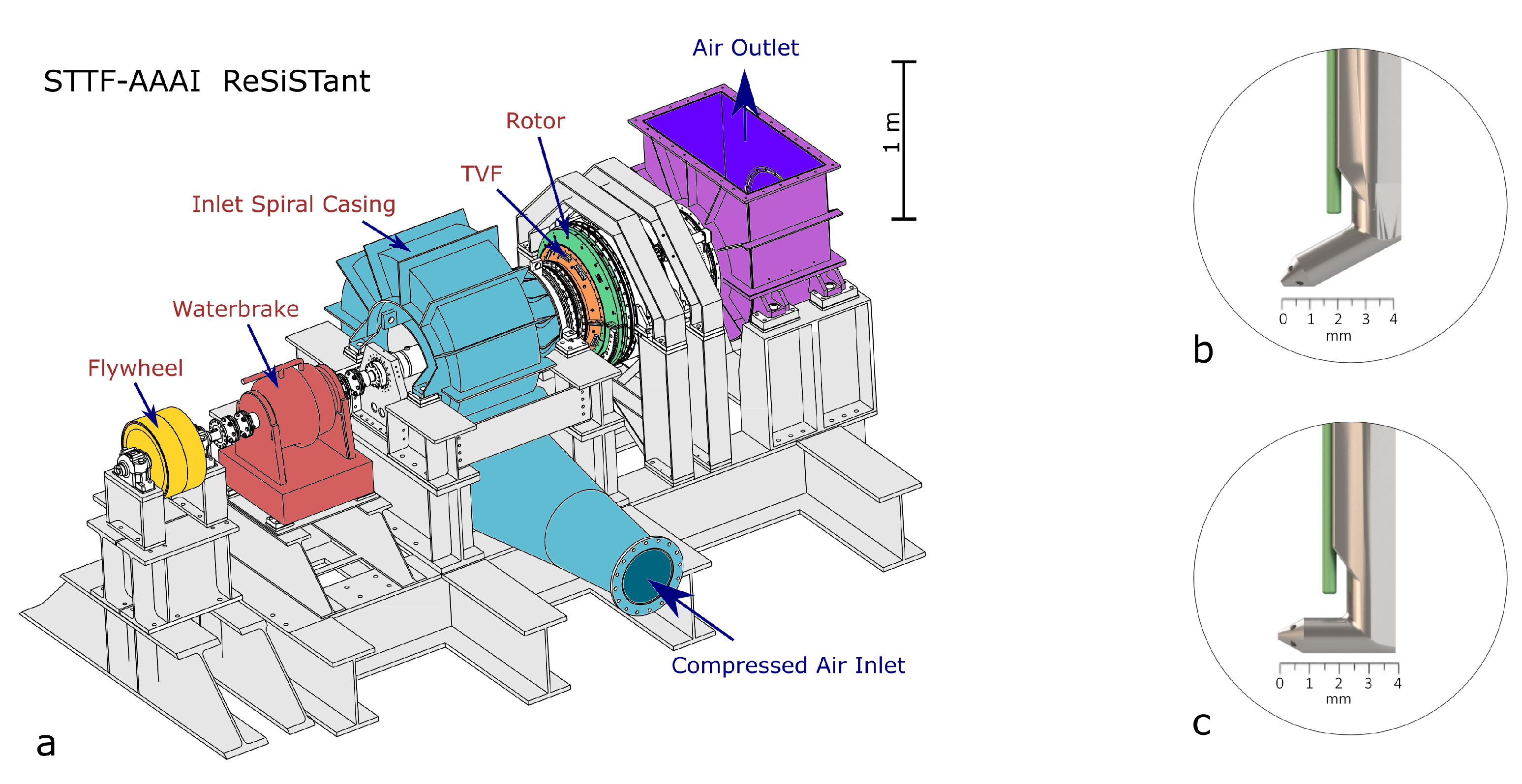
At the Institute for Thermal Turbomachinery and Machine Dynamics (ITTM) at the Graz University of Technology, multiple test turbine facilities are operated to investigate different parts of aero-engines. One of these test facilities is the Subsonic Test Turbine Facility for Aerodynamic, Aeroacoustic and Aeroelastic Investigations (STTF-AAAI), which was used for the investigations in the present paper. In the framework of the ReSiSTant project, big parts of the test facility were changed. While for past projects, it was used to test the last stage of an LPT and different turbine exit casings (TEC), it is now used to test a TVF and the first stage of an LPT. Thanks to the facility’s modular design, core components like the inlet casing, the waterbrake, the flywheel, and the outlet casing did not have to be changed.

The design of the test facility also allows for a complete change from the TEC setup to the TVF setup within a few days. Such fast swaps of setups can only be performed because the bigger parts of the TVF setup assembly are conducted outside the testrig. The TVF assembly incorporates a complete shaft with bearings, oil supply, and vibration monitoring system supporting the LPT. This assembly can then be installed on the test facility using a crane, and the shaft of the LPT and the waterbrake can be connected by a coupling.

Figure 1 shows a cross-section, and Figure 2a an isometric view of the test facility. Air from a compressor station enters the testrig through an inlet spiral casing with deswirler vanes, which turn the flow into the axial direction and allow for a uniform flow field in the circumferential direction. Downstream of the spiral casing, a perforated plate with a porosity of 0.58 and hole diameters of 8 mm is located to further equalize flow inhomogeneities before the air flows through the investigated components. In the present case, those components are a TVF with splitter vanes and an LPT with a shrouded tip. Further downstream, a set of outlet guide vanes is located to turn the flow in the axial direction again. Finally, the air passes two sets of struts—necessary for structural reasons—and leaves the testrig through the exhaust casing.

The test facility features five circumferentially traversable measurement planes for all kinds of aerodynamic probes depicted with red lines and letters (B, C, D, E, and F) in Figure 1. Downstream of the perforated plate, a non-traversable measurement plane (Plane 0) equipped with combi-rakes for total pressure and total temperature used to set the operating point of the test facility is located. Further, more than 1200 static pressure taps located at the endwalls and the airfoils of the TVF vanes are integrated into the test facility. A telemetry system is attached to the downstream end of the rotor shaft to perform vibration measurements of the rotor blades.

A waterbrake is used to break the turbine rotor. The flywheel with a mass of 400 kg depicted on the left side in the isometric view is used to stabilize the shafts’ rotational speed and to reduce the rotating parts’ accelerations in case of brake failure. The testrig is supplied by compressed air generated by a compressor station consisting of two radial compressors and a rotary screw compressor with a combined peak electrical power consumption of 3 MW. A heat exchanger and a recooling system are used to reduce the temperature of the air coming from the compressor station. With a set of valves, the air flowing through the heat exchanger can be controlled to adjust the air temperature at the inlet of the testrig.

The measurements for the present paper were carried out using different five-hole probes with thermocouples. The five-hole probe with a 90${}^{°}$ head depicted in Figure 2b was used for the measurements in planes C and D, and the probe with a 120${}^{°}$ head depicted in Figure 2c was used for the measurements in planes B, E, and F.

2.2. Numerical Setup

For the numerical simulations, an element-based finite volume method with a commercial fully implicit coupled solver was used. The system of equations is solved in an iterative way using a multigrid accelerated factorization technique. More details on the solver can be found in [11].

As a working fluid, air with properties of state of an ideal gas and viscosity according to Sutherland’s Law was chosen. Conservation equations were solved for mass, momentum, energy, turbulent kinetic energy, and specific turbulence dissipation rate. As a turbulence model, the two-equation SST k-$\omega$ eddy viscosity model developed by Menter [12] was used. Additionally, the modification of the production term of the turbulence model called Curvature Correction, suggested by Spalart and Shur [13], was used.

The numerical mesh consists of two domains: The first domain, containing the TVF and the splitter-vanes, starts immediately downstream of the perforated plate and ends shortly upstream of the LPT. The second domain starts where the first domain ends, and ends shortly upstream of the deswirler-vanes. The second domain is located in the rotating frame of reference. The dashed lines in Figure 1 represent the boundaries of the numerical domains. The numerical mesh was created using an in-house mesh generator and consists of about two million hexahedra elements for one passage of the TVF and about 0.6 million for one passage of the LPT. The mesh features yplus values of around three and inflation ratios of around 1.1 normal to the walls in the boundary layers. A mesh-independence study was performed using meshes with different sizes and different mesh generators. In this paper, the described results were found to be independent of the used meshes.

As boundary conditions at the inlet, the total pressure and the total temperature distributions obtained from measurements at measurement plane B were used. The inlet flow direction was chosen to be parallel to the endwalls and zero in the circumferential direction. The turbulence intensity used for the final simulation was determined iteratively so that the turbulence intensity of the CFD calculation in plane B matches the turbulence intensity measured using a hot-fiber-film probe in the same measurement plane. The turbulent length scale has a value of 8 mm, corresponding to the diameter of the holes of the perforated plate upstream of the inlet. At the outlet, a static pressure profile distribution obtained from another CFD simulation containing also the deswirler vanes downstream of the rotor was used. At the endwalls and airfoils, adiabatic no-slip boundary conditions were used.

For the steady-state simulations, a mixing-plane interface was used between the TVF and the LPT. A mixing plane is a common approach to reduce computational resources by averaging the flow variables in the circumferential direction. Consequently, only one passage needs to be simulated for each domain. However, the downside of this approach is that no wakes or other flow structures are transported to downstream components. Therefore, additionally, transient simulations using a profile transformation interface were performed. In the literature, transient simulations are also called unsteady RANS or URANS. This interface allows for a simulation of two domains with slightly different angular sectors in the circumferential direction by stretching one of the domains. To keep the scaling of the interface minimal, multiple instances of LPT blades were used so that the difference between the angular sectors was small. More information on the interface can be found in the manual of the solver [11]. For the transient simulations, 100 timesteps per period were solved.

2.3. Operating Points

For the investigation of the turbine vane frame, measurements and simulations at three operating points have been performed. The first operating point is called aero design point (ADP), and represents the operating point with the lowest losses. For a real engine, this is usually during cruise flight. The second operating point is called cutback (Cut). For a real engine, it represents the operating point after the climb, when the pilot reduces the power of the engine for legal reasons due to noise. Compared to ADP, the inlet Mach number and the rotational speed of the rotor are lower. The last operating point is called approach (App), and represents landing. The inlet Mach number is similar to cutback. However, the inlet total temperature and the rotational speed of the rotor are reduced by about half.

3. Results

3.1. Comparison Experiment: CFD

One goal of the present study was to use the CFD simulations to understand better the flow structures and the different loss mechanisms of the TVF. Therefore, a good agreement between experiment and simulation is necessary. Different types of measurements and visualizations were performed to compare experimental data and CFD.

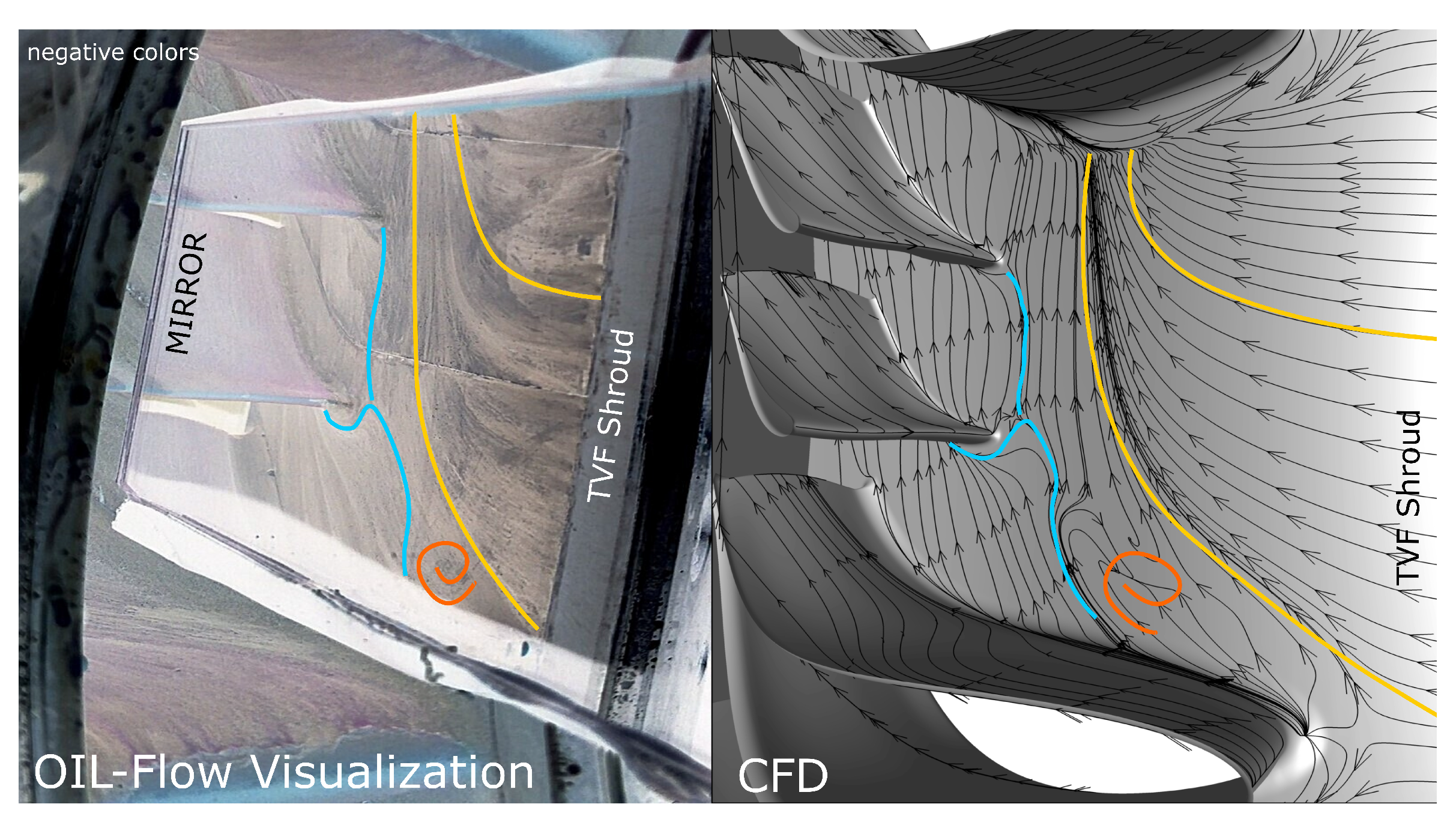
For a qualitative comparison of the trajectories of the wall shear stress at the endwalls, oil-flow visualizations were performed in the test facility. In the left image in Figure 3, the results of the oil-flow visualization are reported. For better visibility of the trajectories, the colors of the original image were inverted. As a result, dark areas show locations with a higher amount of mixture on the surface, which means a lower wall shear stress. A mirror was used to take the reported photography to obtain a better view of the shroud surface.

By enabling the curvature correction described by Spalart and Shur [13], the strong turn of the trajectories of the wall-shear stress marked with yellow lines in Figure 3 and the separation marked with an orange line could be reproduced by the CFD simulation.

For a further comparison of CFD and experiment, plots of the spanwise distributions in the three measurement planes for the total pressure and the Mach number are reported in Figure 4. The values are normalized with the average of the values of each plot. The bars at the bottom of the figure indicate the max uncertainties of the measurement results.

For the Mach Number, a good agreement was observed in measurement panes B and C. For those measurement planes, no significant differences in the profiles for the different operating points are present. In measurement plane D, the experiment shows fewer distinct peaks near the endwalls. Next to the hub, the transient simulation shows a better agreement with the experiment.

The total pressure profile of the simulation in plane B matches the profile of the experiment, since it was used as a boundary condition at the inlet. In plane C, the simulation was able to capture all the major structures visible also in the measurement. However, also here, the structures are more pronounced in the CFD. As expected, no significant differences between steady-state and transient simulations can be observed in the measurement planes upstream of the rotor. In measurement plane D, also for the total pressure, a better agreement of transient simulation with the experiment can be observed. In this plane, the spot with lower total pressure at around 80$\%$ span for all operating points captured by CFD is not visible in the measurement results.

3.2. Losses in the Turbine Vane Frame

To describe the spatial location of losses in the TVF and some of the mechanisms causing them, different graphs are represented in Figure 5. The graphs in Figure 5a represent the following data:

• The dash-dotted graphs show the mass-flow-averaged levels of the total pressure in different slices in the streamwise direction of the TVF for the operating points. They give a rough insight into the pressure levels for the operating points approach, cutback, and ADP, and show how the total pressure levels evolve through the TVF. The pressure levels for approach are the lowest, and the pressure level of ADP is the highest.
• The dots represent the values of the mass-flow-averaged total pressure measured in measurement planes 0 and C in the test facility. For all the operating points the measured total pressure agrees well with the simulation.
• To better understand the mechanisms of the losses, an analytical approach for calculating the pressure drops in the TVF using Darcy friction factor formulae was added to the graph as a dashed line. The pressure drop was calculated for multiple slices in the streamwise direction using the following formula, where p is the pressure, x the streamwise direction, $\lambda$ the friction factor, $\rho$ the density of the flow taken from the numerical simulation, v the mass-flow averaged absolute velocity of the flow taken from the numerical simulation and D the hydraulic diameter calculated for every slice in the TVF.

  $$\frac{\mathrm{d}p}{\mathrm{d}x}=\lambda \frac{\rho v^2}{2D}$$
  The friction factor $\lambda$ was calculated using Blasius’ equation for turbulent flow (Blasius [14]), where $Re$ represents Reynold’s Number calculated for every slice in the TVF.

  $$\lambda =\frac{0.3164}{R{e}^{0.25}}$$
• Finally, the percentage of the areas with backflow in the TVF are represented as solid lines, since they were found to have a significant impact on the losses in the TVF. The backflow was calculated by integrating the areas in each slice in the streamwise direction where the velocity vector is pointing against the direction of the main flow. The areas below the graphs represent the volume of separated flow in the TVF. Areas with backflow are located at the leading edges of strut and splitter vanes and also at the trailing edges. At those locations, the amount of backflow is similar for all operating points. However, the largest areas with backflow are located downstream of the leading edges of the strut vanes at a streamwise location of around $0.7$. These areas are also visible in Figure 3 and are marked in orange. The simulation shows the separation to differ in size for the different operating points.

Figure 5. Losses in the TVF over the streamwise direction. (a) shows the total pressure and the amount of backflow for the three operating points ADP, approach, and cutback over the streamwise direction. The dash-dotted lines represent the total pressure of the CFD results, the dashed lines represent the total pressure calculated according to Darcy’s model, and the dots represent the total pressure from the experiment. The solid lines represent the amount of backflow in for the corresponding streamwise location. (b) shows the pressure loss coefficients for the three operating points for the CFD, the analytical model, and the experiment over the streamwise direction. The graphs for the different operating points are almost perfectly collapsed. (c) shows the streamwise gradients of the pressure loss coefficients for the three operating points for the CFD and the analytical model over the streamwise direction. The graph indicates the amount of losses in each streamwise position.

Figure 5. Losses in the TVF over the streamwise direction. (a) shows the total pressure and the amount of backflow for the three operating points ADP, approach, and cutback over the streamwise direction. The dash-dotted lines represent the total pressure of the CFD results, the dashed lines represent the total pressure calculated according to Darcy’s model, and the dots represent the total pressure from the experiment. The solid lines represent the amount of backflow in for the corresponding streamwise location. (b) shows the pressure loss coefficients for the three operating points for the CFD, the analytical model, and the experiment over the streamwise direction. The graphs for the different operating points are almost perfectly collapsed. (c) shows the streamwise gradients of the pressure loss coefficients for the three operating points for the CFD and the analytical model over the streamwise direction. The graph indicates the amount of losses in each streamwise position.

In Figure 5b, the total pressure coefficients $C_{pt}$ for the data from Figure 5a were calculated using the following formula, where $p_t$, $p_{t0}$ and $p_0$ are the total pressure at the correspondent streamwise location, the total pressure in plane 0, and the static pressure in plane 0, respectively.

$$C_{pt}=\frac{p_{t0}-p_t}{p_{t0}-p_0}$$

When applying this equation, the graphs of the different operating points collapse, meaning the losses mostly relate to the flow velocity at the inlet. This is true for the CFD solution and the analytical solution, as well as the measurement. The graphs for the CFD solution show higher pressure losses than the analytical solution, which is not a surprise since the analytical solutions only take the pipe losses into account. The measured losses appear again higher than the losses predicted by the CFD. The absolute difference between the experiment and the simulation is small, however, since the overall pressure loss in the TVF is also small. The differences in the pressure losses for the experiment for the different operating points lie within the measurement accuracy.

To compare the losses in more detail, in Figure 5c, the gradients of the graphs from Figure 5b are represented. Comparing the analytical solution of the pipe loss with the CFD solution, some similarities can be observed. High gradients are present at the leading and trailing edges of the vanes, where separations occur and the wetted surface increases. A decrease in the gradients occurs downstream of the struts leading edges, where the flow decelerates. High gradients are located upstream of the trailing edges, where the flow accelerates due to the turning of the vanes. Starting at the streamwise location of $0.9$ for the CFD solution, the graphs start to diverge, which can be explained by the different sizes of the separations observed in Figure 3 and Figure 5a. The separations increase the strength of the vortex structure shown with yellow lines in the figure of the oil-flow visualization. However, the vortex structure gets transformed into losses only as soon as the flow accelerates downstream of the splitters’ leading edges.

3.3. Differences between the Operating Points

To describe the differences between the operating points, different contour plots of the normalized total pressure in measurement plane D are reported in Figure 6. The upper plots show the simulation, while the lower plots show the experiment. The first column of plots shows the normalized Mach Number of the operating point ADP. Both simulation and experiment show similar structures of the flow field at similar levels. The same plots for the other two operating points are not reported here since, as already described in the previous section, the flow fields for the different operating points are very similar. Instead, plots with the difference of the pressure coefficients $C_{pt}$ and the yaw angles ${\alpha }_{yaw}$ of ADP and approach are reported in the figure.

The most prominent vortices present in this measurement plane are marked in the plot. For all three wakes, a similar wake structure with the same vortices can be observed. However, for the wake of the strut, the upper passage vortex (PV) is positioned at a much lower spanwise position and causes a large loss core. This vortex is increased by the separation and the yellow vortex structure, shown in the oil-flow visualization. For all the wakes, a good agreement of experiment and simulation can be observed. The CFD was able to capture all the main vortices and loss cores.

As shown in Figure 5b, the differences of $C_{pt}$ between ADP and cutback are very small. However, Figure 6c,d show a good agreement of simulation and experiment also for these small quantities. The $C_{pt}$ is higher for the ADP at the pressure sides, while it is lower at the suction sides. The biggest differences between the operating points can be observed in the regions where multiple vortex structures collide in the wakes close to the endwalls. It can therefore be concluded that the mechanisms forming the vortices are affected by the different operating points.

As shown in Figure 6e,f, the differences in the yaw angle between ADP and cutback are only small, but a good overall agreement between simulation and experiment can be observed. The flow turns stronger for ADP than for cutback, which has a lower flow velocity. Other than for the pressure loss coefficient, the differences between the operating points are present in the whole section and not only in the wakes. The spanwise location of the areas with bigger differences differs between the passages of the TVF. While the area with larger flow angles is located closer to the shroud for the passage at the pressure side of the strut, it is located closer to the hub for the passage between the two splitter vanes. In that passage, even an area with larger flow angles for cutback is visible in the contour plots.

More details on the secondary flow inside this TVF were published in Pramstrahler et al. [5], [6].

3.4. Losses in the Low-Pressure Turbine

The rotational speed of a turbine influences the velocity triangles and the angle of attack of the blades. This usually has a strong impact on the performance of the low-pressure turbine. In the case of the investigated setup, the performance of the low-pressure turbine is additionally dependent on the different wake signatures of the TVF, compared to a conventional vane row, with a higher number of vanes.

In Figure 7, contour plots of the normalized total pressure for the three operating points from five-hole probe measurements are represented. The data were normalized using the mass-flow averaged total pressure for each measurement. The blue areas in the plots are locations with lower total pressure and come from the wakes of the TVF vanes, which travel through the rotor. As in measurement plane C, also here in measurement plane D, the wake of the strut is the most prominent. For all operating points, it consists of two loss cores and is located at lower span heights compared to the loss cores originating from the wakes of the splitter vanes. Further, for all operating points, the loss cores of splitter 1 are stronger than the loss core of splitter 2. Comparing the operating points, the loss cores are positioned at different circumferential positions, which can be explained using the velocity triangles. For all the operating points, the yaw angle downstream of the LPT is negative (see Figure 1 for a definition of the angles). For the operating point cutback, the circumferential velocity component downstream of the LPT is the smallest, and for the operating point approach, it is the largest. The different circumferential and axial velocities cause different static pressure distributions downstream of the rotor for the tested operating points. As a result, the spanwise location of the areas with higher levels of total pressure marked with the letters X, Y and Z change. For larger yaw angles, they are pushed more strongly toward the hub. Especially for the operating point approach, the area marked with the letter X extends over a big area of the span and pushes the loss cores originating from the strut wakes toward the hub.

In Figure 8, the normalized total pressure from the transient numerical simulation for the operating point ADP in plane D is shown. In Figure 8a, the data were time-averaged, and in Figure 8b, a single time frame of the simulation is shown. Surprisingly, the differences between the two plots are quite small, and the wakes of the rotor blades are almost not visible. The biggest differences can be seen in the areas with higher total pressures marked with the letters X, Y and Z. In areas with low total pressure, almost no differences can be spotted comparing the two plots.

Comparing the measurement from Figure 7a and the experiment from Figure 8a, a good overall agreement can be observed. The CFD was able to capture all the most prominent structures. The biggest differences between CFD and the experiment are at the shroud, where the experiment shows areas with lower total pressure. By simulating the cavities of the shrouded rotor blades, the agreement of CFD and experiment could probably be further improved in this area.

4. Conclusions

In this study, a turbine vane frame and a low-pressure turbine rotor were investigated experimentally and numerically. A detailed comparison of the losses inside the TVF for three different operating points was performed, and the differences were described. It was shown in which streamwise location the losses occur in the TVF, and that the total pressure coefficient is similar for all the investigated operating points. Further, a simple analytical method using the Darcy friction factor was used to find the locations with the highest losses in the TVF. Differences between the operating points have been observed in the wakes and for the yaw angles downstream of the TVF. Downstream of the LPT, the flow structures are mainly influenced by the rotational speed of the rotor. However, the wakes of the TVF have a stronger impact on the flow field than the wakes of the LPT blades in measurement plane D downstream of the LPT.