Article

Turbulence Measurements Downstream of a Combustor Simulator Designed for Studies on the Combustor–Turbine Interaction †

Department of Energy, Politecnico di Milano, 20158 Milano, Italy
*
Author to whom correspondence should be addressed.
This manuscript is an extended version of the ETC2023-323 meeting paper published in the Proceedings of the 15th European Turbomachinery Conference, Budapest, Hungary, 24–28 April 2023.
Int. J. Turbomach. Propuls. Power 2024, 9(1), 4; https://doi.org/10.3390/ijtpp9010004
Submission received: 25 September 2023 / Revised: 13 October 2023 / Accepted: 1 December 2023 / Published: 10 January 2024

Abstract

:
Turbulence intensity impacts the performance of turbine stages and it is an important inlet boundary condition for CFD computations; the knowledge of its value at the turbine inlet is then of paramount importance. In combustor–turbine interaction experimental studies, combustor simulators replace real combustors and allow for the introduction of flow perturbation at the turbine inlet. Therefore, the turbulence intensity of a combustor simulator used in a wide experimental campaign at Politecnico di Milano is characterized using a hot-wire probe in a blow-down wind tunnel, and the results are compared to URANS CFD computations. This combustor simulator can generate a combination of a swirl profile with a steady/unsteady temperature disturbance. In the cold unsteady disturbance case, hot-wire measurements are phase-averaged at the frequency of the injected perturbation. The combustor simulator turbulence intensity is measured at two different axial positions to understand its evolution.

1. Introduction

To reduce pollutant emissions of gas turbines for both propulsive and stationary applications, combustors are designed to burn a lean-premixed mixture. In addition, a strong swirl is imposed on the combustion air to enhance air–fuel mixing and stabilize the flame. Lean-burn combustors release a flow field characterized by unsteady temperature and velocity inhomogeneities in both the radial and circumferential directions. Especially in aeroengines, where compactness is required, such inhomogeneities move downstream until the first turbine stage and, notwithstanding an attenuation in the combustor duct, they impact blade aerodynamics, blade cooling effectiveness [1], and combustion noise [2].
As such an impact cannot be neglected, several experimental and numerical investigations have been performed to identify, describe, and quantify it, with the aim of improving the control of the combustor–turbine interaction [3,4,5,6,7,8,9].
In this context, many combustor simulators (used by [5,7]) have been conceived to mimic the combustor-released flow using non-reactive devices, which allows experimental testing and numerical simulation.
As demonstrated by Khanal et al. [3], individually considering combustor non-uniformities is questionable because the nonlinearity of the process prevents a straightforward superposition of the effects. In addition to these features, the unsteadiness of the temperature pattern makes the study much more complex and requires a dedicated combustor simulator for running experiments. As a matter of fact, nowadays there is a growing interest in studying the combined injection of a swirl profile and hot streaks/entropy waves [3,4,5,6,7,8,9]. Several experimental campaigns have been performed at Politecnico di Milano since 2015 [10], focusing on the transport of entropy waves within an HP turbine stage. The most recent combustor simulator used to generate turbine-inlet non-uniformities was conceived to combine a swirl profile and entropy waves [9]. Such an inlet flow field makes this experimental campaign one of a kind. The results of this wide experimental campaign were partially described in [9,11], and the interested reader is invited to refer to these studies for detailed results.
In the aforementioned papers, information about the turbulence of the flow at the turbine inlet was missing due to the mechanical constraints of the turbine rig that did not allow for the insertion of a hot wire, commonly considered the primary tool for such measurements. As found by previous authors [12,13,14], turbulence intensity impacts turbine loss mechanisms and increases heat transfer. Therefore, this is an important feature that has to be reproduced by combustor simulators. In fact, combustor outlet turbulence can exceed 10% [15,16,17], which is a much higher value than what can be achieved using grids. In [18,19,20], the turbulence intensity generated by combustor simulators was studied. This paper aims to describe the turbulence field released by the combustor simulator used in [9] and its decay as the stream propagates downstream. Experiments were performed at different injection conditions and different distances from the injector. In addition, RANS CFD simulations were carried out to support the physical interpretation and integrate the results of the experimental campaign.

2. Materials and Methods

To investigate the turbulence generated by the combustor simulator used on the turbine test rig at Politecnico di Milano, the simulator is placed in a blow-down wind tunnel that can replicate turbine inlet conditions by imposing the same Mach number. However, due to density effects, the Reynolds number is 30% lower in this setup. Table 1 provides information regarding the mainstream properties. Considering the different flow features, three Reynolds numbers are given: Reduct is computed based on the duct size, Rec,swirler is computed based on the chord of the swirler generator blades, and Red,injecotor is computed based on the injector diameter. The calibrated nozzle of the wind tunnel is fed by compressed stored air and has a 0.08 m square exit section. According to the nozzle calibration, the open jet generated retains a wall-bounded character for an axial distance of two jet widths downstream of the nozzle. The combustor simulator is placed within a straight prolongation added downstream of the exit section (Figure 1). This device includes a swirler generator (highlighted with a circle in Figure 1) that can inject steady/unsteady temperature disturbances. Probes are traversed downstream of the device at two traversing planes: one representative of the plane where measurements are carried out upstream of the turbine stage, which is approximately one chord of the swirl generator blade downstream of the device itself, and the second at a position coincident with the turbine vane LE (in the turbine experiments). Both the planes are inside the axial extension of 2 jet widths. The characterization of the turbulence generated by the combustor simulator is carried out using a slanted hot-wire probe. In addition, a 5-hole probe is used to assess the hot-wire measurements.

2.1. Generated Combustor Disturbances

The combustor simulator allows for studying several steady/unsteady injection cases. In the steady cases, a by-pass valve is opened and only one duct, labeled “duct 1” in Figure 1, is continuously fed. To simulate this condition in CFD, the inlet plane of duct 2 is treated as a wall. In the unsteady cases, a set of automotive valves is used to alternatively feed the two different ducts that are then rejoined at the head of the injector (Figure 1). The air flowing in duct 1 can be heated by an electric heater. At the outlet of the injector, a swirl generator is placed, which acts on both the mainstream air and the steady/unsteady generated disturbances. Further details of the combustor simulator are described in [9].
Flows at ambient temperatures are necessary for hot-wire measurements because temperature affects the hot-wire calibration, and a too-high temperature can burn the wire. As such, the combustor simulator electric heater is switched off and hot cases are only simulated through CFD. Table 1 lists and defines the four injection cases studied. The first case, hot streak (HS), involves a steady injection of a hot flow into injector duct 1. In the second case, referred to as cold streak (CS), duct 1 is fed with a steady flow at an ambient temperature. The third case, entropy wave (EW), features an alternate injection of hot and cold flows in ducts 1 and 2, respectively. Lastly, in the unsteady CS, ducts 1 and 2 are fed alternatively, as in the EW case, but the flow in duct 1 is at an ambient temperature. The feeding pressure of the injector ducts used in turbine tests [9] is rescaled on the basis of the different pressure ratios.

2.2. CFD Setup

A dedicated, fully 3D URANS computational model was developed in the ANSYS-Fluent framework, considering the injector of the combustor simulator immersed in the nozzle airflow. Figure 2 shows a schematic of the boundary conditions. The inlet boundary is placed at the nozzle outlet section. Two further inlet conditions are placed at the head of the injector, where steady/unsteady boundary conditions are set. The inlet boundary conditions include the temperature and velocity magnitude, while the static pressure is specified at the outlet. The injector surfaces are modeled as no-slip walls, and the domain’s four lateral surfaces, i.e., the lateral surfaces of the jet, are modeled as slip walls. According to measurements, at the inlet, the turbulence intensity is assigned equal to 1%, and the turbulence length scale is also assigned at 10% of the relevant inlet boundary scale.
Unsteady RANS CFD simulations are also carried out for the steady injection cases to simulate the vortex shedding downstream of the injector stem, which should play a significant role in the decay of the main properties of the perturbation generated by the simulator. After performing an FFT on the instantaneous mass-flow average at the outlet section, the main periodicity of the problem is identified, and the period is discretized into 40 time steps.
Figure 2 shows a cut of the unstructured 3D mesh. Two meshes are tested, and the results of a grid-independence analysis are shown in Table 2. The two meshes feature the same boundary layer resolutions, characterized by 20 layers and a y+ < 1. The mesh is not further coarsened to accurately catch the mixing that occurs downstream of the injector. Among the two tested meshes, the one with 6 million cells is used, considering the small differences in the outcomes of the grid-independence analysis shown in Table 2.
After several preliminary trials changing numerical schemes, the fluent pressure-based coupled solver is selected, using the k- ω SST turbulence model and the ideal gas as a thermodynamic fluid model. High resolution in the numerical solution is achieved by adopting second-order upwind schemes for the advective fluxes, second-order central differences for the viscous terms, and the second-order implicit discretization of the unsteady term.

2.3. Measuring Technique

This section describes the measurement techniques utilized during the experimental campaign. The pressure drop across the nozzle is measured using a KuliteTM XT190 transducer (Leonia, NJ, USA), which has a full scale of 5 psi. The outlet pressure is the ambient pressure that is read by a FisherTM (Drebach, Germany) model 104 barometer with an average uncertainty of 50 Pa calibrated in the LAT n° 024. In order to phase-average the hot-wire measurements at the frequency of the injected disturbance, the pressure in injector duct 1 is used as a trigger signal and is measured using a KuliteTM XT190 transducer with a full scale of 25 psi. The transducer’s maximum uncertainty is 0.05% of its full scale. The measuring signals are acquired using a National Instrument data acquisition board (PCI 6052E) with a range of ±10 V.
Temperatures are measured using thermocouples: the nozzle supply air temperature is measured using a T type, whereas the injector ducts and ambient temperature are measured using a K type. Temperature uncertainty after calibration is 0.3 °C.
At the traversing planes, a 5-hole probe and a hot-wire anemometer are used.

2.3.1. Five-Hole Probe

A 5-hole pressure probe is used to characterize the steady aerodynamic flow field at the two traversing positions. The probe head has a diameter of 2.2 mm and an overhang of 5 mm.
The probe is aerodynamically calibrated in a Mach number range of 0.1–0.3 and an angular range of ±44° both in pitch and yaw angles, chosen to proficiently characterize the complex 3D field. The yaw angle is the angle around the probe axis, and the pitch angle is the angle of inclination of the probe axis with respect to the main flow direction. The average uncertainties of the 5-hole probe are calculated using the Monte Carlo method described in [21], which predicts an average extended uncertainty of 1.5° for angles, 2.5 m/s for absolute velocity, and 100 Pa for pressure.

2.3.2. Hot-Wire

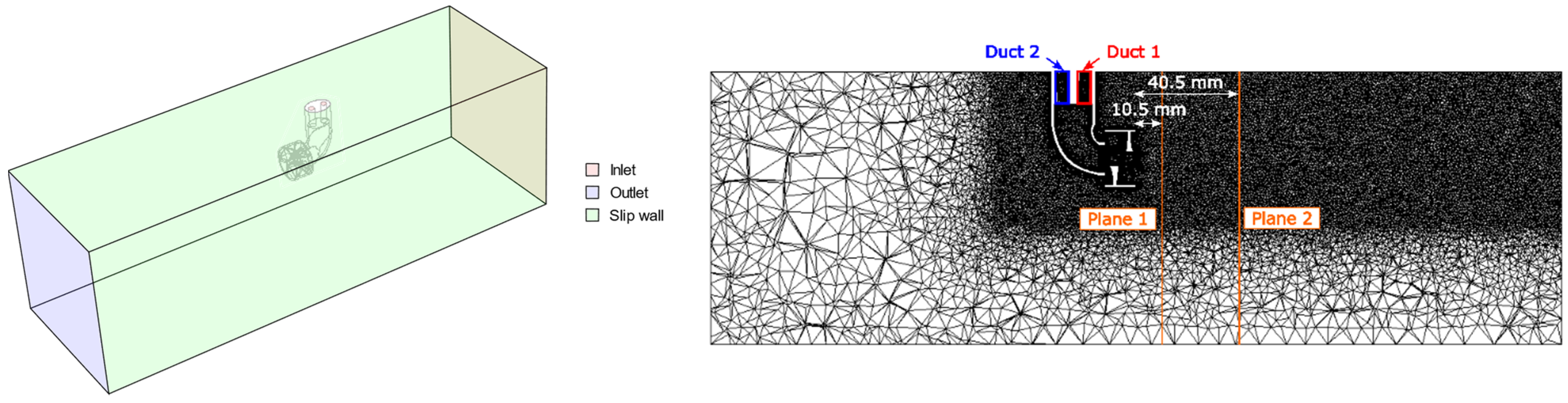
The hot wire used in this experimental campaign is a slanted single-sensor probe with a slanting angle of 45° that is connected to a DISA55M system. The wire diameter of ~5 µm guarantees a very high dynamic response (~30 kHz) in the constant temperature configuration, making this probe suitable for measuring the turbulence structures of both low- and high-speed flows. The probe is mounted on four stepping motors (Figure 1): two control the traversing position, one controls the yaw angle, and one controls the pitch angle.
To keep the wire temperature constant in the presence of an incoming flow, the hot-wire Wheatstone bridge regulates the supply voltage. This well-established response relationship is described by King’s law:
E ¯ c o r r 2 = A + B Q n
where E ¯ c o r r is the mean average of the supply voltage, once corrected to account for temperature drifts; Q is the cooling velocity; and A , B , and n are the calibration constants obtained after a least-square regression of the calibration data. In King’s law, the hot wire is aligned perpendicularly to the main flow so that the cooling velocity Q corresponds to the flow velocity U . In the case of a slanted single-wire probe, this condition is achieved by placing the probe at a pitch angle of −45° and a yaw angle of 0°. In this way, the cooling velocity depends only on the normal component of the flow velocity, and the other velocity components are null; in all other cases, one would need to know the angular sensitivity of the probe, which is normally still unknown at this stage of the calibration. Another constraint for determining King’s law is that the turbulence intensity of the calibrating jet is small (below 5%) because, as shown later, the velocity also depends on the Reynolds tensor components. Both these conditions were properly matched in the calibrations performed for this study.
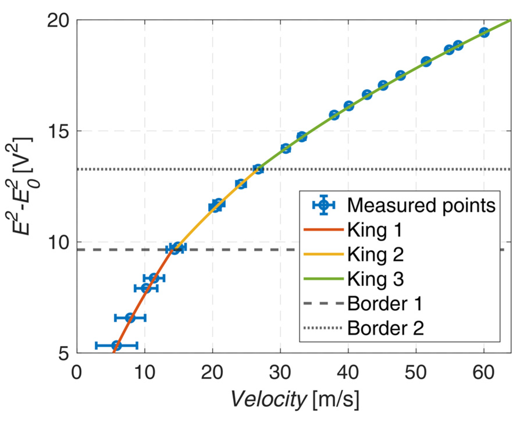
The methodology applied in this work requires careful discussion, as specific actions are taken to improve the results’ reliability. First, King’s law is split into three different voltage ranges (Figure 3) to improve the accuracy of the interpolation. Second, the anemometer output signal E is corrected to account for possible temperature drifts during the calibration using Equation (2), as suggested by Bruun [22]:
E c o r r 2 = E 2 T w T 0 T w T f l o w E 0 2
T w is the constant temperature of the wire (set at 493 K), T 0 is the temperature at which the voltage zero E 0 is performed (at rest conditions), and T f l o w is the temperature of the incoming air.
The fluctuating component of the cooling velocity is derived by decomposing King’s law [23]. It depends on the King’s coefficients and the mean velocity:
q 2 ¯ = 2 E ¯ c o r r n B Q ¯ n 1 2 e 2 ¯
where q   is the fluctuating velocity component and e is the root mean square of the hot-wire voltage measurements.
In real applications, the actual velocity could not be perpendicular to the wire. In this case, the other velocity components impact the cooling velocity of the hot wire in a non-linear way. The influence of these velocity components on the cooling velocity is well described by Jorgensen’s law [23]:
Q 2 = U n 2 + k 2 U t 2 + h 2 U b 2
where n is the normal component, t is the tangential component, and b is the binormal component with respect to the wire (Figure 1). h 2 and k 2 are the two angular calibration coefficients to be defined through an aerodynamic calibration. It must be emphasized that in the definition of King’s law, only the normal component is not null. In fact, the change in the reference system from the hot wire to the nozzle yields:
U n = U ( c o s θ c o s φ s i n α s i n θ c o s α ) U t = U ( c o s θ c o s φ c o s α + s i n θ s i n α )   U b = U c o s θ s i n φ
In the literature, the coefficient k 2 is available for standard probes [24]. In this paper’s application, the choice is to carry out a calibration to also determine the k 2 coefficient by varying the pitch angle. For this purpose, the hot-wire yaw angle is set to zero, that is, U b = 0, and the pitch angle is varied within the calibration range of ±45° every 5°. This is possible after verifying that the dependence of k 2 on the yaw angle is negligible. The k 2 coefficient can be computed according to Equation (6) by imposing the yaw angle φ = 0 ° .
k 2 = Q 2 U 2 c o s θ s i n α s i n θ c o s α c o s θ c o s α + s i n θ s i n α
The last angular calibration coefficient h 2 can be calculated, as shown in Equation (7), by imposing different combinations of the yaw and pitch angles. For each pitch angle, the yaw is moved within the range of ±120° every 5°.
h 2 = Q 2 U 2 c o s θ c o s φ s i n α s i n θ c o s α 2 k 2 c o s θ c o s φ c o s α + s i n θ s i n α 2   c o s θ s i n φ 2
Once the calibration coefficients are defined, the probe can be applied in an unknown flow field to reconstruct its velocity components and the turbulence content. The flow velocity can be decomposed into its three components in the x-y-z reference system that can be correlated to the hot-wire reference system components using Equation (8), where φ r o t is the rotation of the yaw motor.
U n = U 1 c o s α + U 2 c o s φ r o t s i n α + U 3 s i n φ r o t s i n α U t = U 1 s i n α + U 2 c o s φ r o t c o s α + U 3 s i n φ r o t s i n α U b = U 2 s i n φ r o t U 3 c o s φ r o t
Therefore, the cooling velocity can be related to the velocity components in the nozzle reference system by substituting Equation (8) into Equation (4):
Q 2 = A 11 U 1 2 + A 22 U 2 2 + A 33 U 3 2 + A 12 U 1 U 2 + A 23 U 2 U 3 + A 13 U 1 U 3
The A coefficients depend on the yaw angular position and the slanted angle, as well as the calibration coefficients h 2 and k 2 . One single equation is not enough to solve the flow field due to the presence of three unknowns. To obtain reliable results, the system is overdetermined using 13 equations, calculated by varying the probe yaw angle within the range of ±120° every 20°. This set of angles is chosen after proper validation of the procedure, considering different ranges and angle steps. The overdetermined problem is resolved using a Matlab iterative script and the lsqnonlin function. The first estimation for the velocities is a vector [0; Q; 0], where Q is computed using King’s law.
This procedure is valid in the case of low-turbulence intensity flows because the effective cooling velocity depends on the fluctuating components. By expressing each velocity component in terms of mean (denoted with upper-case letters) and fluctuating (denoted with lower-case letters) components, after calculating the mean value (denoted with an overline), Equation (9) becomes:
Q 2 ¯ = A 11 U ¯ 1 2 + u 1 2 ¯ + A 22 U ¯ 2 2 + u 2 2 ¯ + A 33 U ¯ 3 2 + u 3 2 ¯ + A 12 U ¯ 1 U ¯ 2 + u 1 ¯ u 2 ¯ + A 23 U ¯ 2 U ¯ 3 + u 2 u 3 ¯ + A 13 U ¯ 1 U ¯ 3 + u 1 u 3 ¯
This equation does not allow for the separation of the time mean components and the Reynolds stresses. Equation (10) could be rewritten in terms of both mean and Reynolds stress coefficients, considering the largest velocity component as the one in the axial direction (U2):
Q = A 22 1 2 U 2 ¯   1 + 2 u 2 U 2 ¯ + u 2 U 2 ¯ 2 + A 11 A 22 U 1 ¯ + u 1 U 2 ¯ 2 + A 33 A 22 U 3 ¯ + u 3 U 2 ¯ 2 + A 12 A 22 1 + u 2 U 2 ¯ U 1 ¯ + u 1 U 2 ¯ + A 23 A 22 1 + u 2 U 2 ¯ U 3 ¯ + u 3 U 2 ¯ + A 13 A 22 U 1 ¯ + u 1 U 2 ¯ U 3 ¯ + u 3 U 2 ¯ 1 2
After approximating Equation (11) at the first order, the mean velocity and the mean of its fluctuating component can be derived. The assumption is that all other components are much lower than U 2 ¯ so series expansion can be applied. By further neglecting third-order terms or greater, according to Buresti and Di Cocco [25], the mean effective velocity can be expressed as:
Q ¯ = R 2 U 2 ¯ + R 1 U 1 ¯ + R 3 U 3 ¯ + R 4 U 1 ¯ 2 U 2 ¯ + R 5 U 3 ¯ 2 U 2 ¯ + R 6 U 1 ¯   U 3 ¯ U 2 ¯ + R 4 u 1 ¯ 2 U 2 ¯ + R 5 u 3 ¯ 2 U 2 ¯ + R 6 u 1 ¯   u 3 ¯ U 2 ¯
considering that
q 2 ¯ = Q 2 ¯ Q ¯ 2
By subtracting Equation (10) from Equation (12), properly squared, and neglecting third-order terms,
q 2 ¯ = Z 1 u 2 2 ¯ + [ Z 2 + 2 Z 10 U 1 ¯   U 2 ¯ + Z 12   U 3 ¯ U 2 ¯ ] u 1 2 ¯ + Z 3 + Z 13 U 1 ¯   U 2 ¯ + 2 Z 15   U 3 ¯ U 2 ¯ u 3 2 ¯ + Z 4 + 2 Z 7 U 1 ¯   U 2 ¯ + 2 Z 8   U 3 ¯ U 2 ¯ u 1 u 2 ¯ + Z 5 + Z 8 U 1 ¯   U 2 ¯ + 2 Z 9   U 3 ¯ U 2 ¯ u 2 u 3 ¯ + Z 6 + Z 11 U 1 ¯   U 2 ¯ + Z 14   U 3 ¯ U 2 ¯ u 1 u 3 ¯
The use of these equations is justified by the fact that the turbulence intensity in this application does not exceed 20% [25], making Equations (12) and (14) consistent. In this way, all components of the Reynolds stress tensor can be estimated.
All coefficients (A: Equation (9); R: Equation (12); and Z: Equation (14)) are taken from [24,25], with the only difference being the different reference systems.
However, at the first traversing position, the assumption of U 2 being the dominant velocity is not correct everywhere, especially in the vortex core. If the tangential velocity U 3 becomes dominant, this issue can be easily solved by rotating the reference system: after estimating the velocity direction by resolving the over-constrained system of equations, the central hot-wire rotation is updated to reflect the actual velocity direction. In this way, U 2 again becomes the main velocity component, and the previous equations can be applied. To make this possible, it is necessary to carry out measurements over a wider range of motor rotations to account for possible changes in the reference system. Therefore, for each point, measurements are carried out within the range of ±160°, with ±40° being the maximum/minimum angles expected.
In the case where U 1 is the dominant component, the previous equations are used again but with changes in the procedure from Equation (11) on.
Ultimately, the procedure for resolving the flow field with the hot wire involves the following steps, as shown in the flowchart in Figure 4:
1.
The acquired voltages are used to compute Q ¯ and q ¯ by applying King’s law.
2.
Assuming low-turbulence content and Q = [0, Q ¯ , 0], the mean flow field is solved by iterating Equation (9) over 13 sets of rotations.
3.
The first prediction of the velocity vector is used to update the rotational range and solve the Reynolds tensor (Equation (14)). The updated rotational range is centered on the nearest multiple of 20° relative to the measured yaw angle, encompassing 13 rotations spaced every 20° within the range of ±120° with respect to that closest multiple of 20°.
4.
Considering that the mean velocity depends on the Reynolds stress tensor components (Equation (10)), the assumption made in step 2 is now relaxed. The mean velocity components are recalculated using a least-square regression on Equation (10), utilizing the Reynolds stresses computed in step 3.
5.
With the new mean velocities, the cycle is repeated, starting from step 3 until convergence.
A Monte Carlo simulation is carried out to perform an uncertainty quantification of the HW measurements. Starting from the measuring uncertainties, these are propagated through the whole calibration process. Uncertainties vary depending on the flow regime, with high uncertainties associated with low speed (see Figure 3). The extended uncertainties at a 95% confidence interval are listed in Table 3 for the flow quantities under study.
Figure 4. Hot-wire flowchart.
Ijtpp 09 00004 g004

3. Results

3.1. Steady Cold Streak

The first analysis focused on the validation of the CFD model in the CS case. The validation process involved the analysis of the spanwise profiles of the horizontally mass-averaged quantities at the two traversing planes. The results of this comparison are shown in Figure 5. The CFD and five-hole probe measurements for the total pressure and velocity are compared, both made non-dimensional with respect to the undisturbed mainstream (MS) values. CFD effectively captured the evolution of the lower and upper branches of the swirl profile. The agreement was poorer in the stem wake region, especially at plane 1. The potential main cause of this discrepancy is that the CFD model could not reliably predict the streamwise evolution of the vortexes shed by the injector stem.
To better understand the spanwise profiles in Figure 5, the contour plots for both the experiments and CFD were compared at the first traversing plane in terms of the absolute velocity (Figure 6), streamlines (Figure 7), tangential velocity (Figure 8), and turbulence intensity (Figure 9). All plots were generated from the perspective of an observer placed downstream of the studied plane. In the region of the swirl core at the first traversing plane, both the hot wire and five-hole probe operated near the angular boundaries of their calibration ranges, so some measurements were affected by a higher error. Notwithstanding this problem, the agreement between the measurements and CFD was good. When analyzing the results, two main flow structures were observed. The first corresponded to the wake generated by the injector stem, which is highlighted with a white box in Figure 6 CFD. The second was the swirl profile, which is identified by a white circle. When comparing the CFD results with the experiments, the agreement was good in terms of the velocity magnitude and flow morphology.
Along the circumference of the swirl profile, three regions of high-velocity magnitude were identified, labeled 3, 4, and 5 in Figure 6 CFD. These correspond to the flow released by the swirler generator vanes 3, 4, and 5, as identified in the contour “Plane 0”, which represents the X-Y plane at the swirler generator trailing edge. The other swirler generator channels 1–2 exhibited low velocities because they collected the flow from the injector stem wake. Furthermore, the injected cold streak was swirled mainly by channels 3, 4, and 5, as indicated by the streamlines of the injected streak shown in Figure 7. Being the first measuring plane approximately 10 mm downstream of the swirler generator, the flow structures were not yet completely mixed, thus justifying the presence of velocity peaks. While both probes recorded the three regions labeled 3, 4, and 5, a lower velocity peak was measured, highlighting that the main aim of RANS was to correctly predict the mixing process.
For the same reasons, the tangential velocity contours (Figure 8) show the lowest absolute magnitudes in the left part of the swirl profile, corresponding to swirler generator channels 1–2. The differences between the simulations and experiments are mainly quantitative, as the trends are very similar. Both in the simulations and experiments, a reduction in high positive/negative tangential velocities was observed during the circumferential evolution, which was caused by the wakes of the swirler generator blades.
The agreement between HW and CFD in terms of turbulence intensity is good (Figure 9), which is defined as the ratio of the root mean square of the turbulent velocity fluctuations and the mean velocity. The area-averaged value on the measuring grid in CFD was 7.2% against the 6.1% measured experimentally. These values match the turbulence intensity found by Pinelli et al. [11] in their CFD study. Turbulence was generated downstream of the combustor simulator in the regions of the injector stem wake and swirl core. The region with the highest turbulence intensity was the injector stem wake, which was very well predicted by CFD. In the swirling flow zone, some points of the HW grid were not fully converged because the HW worked close to its angular calibration limits. Despite this, the turbulence intensity levels in the swirl core exhibited a strong match between the simulations and experiments. However, CFD predicted high turbulence in the annular zone contouring the swirl core, which was generated by the shear layer formed at the boundary between the flow released by the swirler generator and the free stream. This feature was not measured in the experiments, probably due to the mixing that took place, nullifying this contribution, which was underestimated by CFD. In both the CFD and HW measurements, the high-velocity zones (3, 4, and 5 in Figure 6) had low turbulence levels. Therefore, the main contribution to turbulence production in this measuring traverse was related to the boundary layers of the injector walls.
At the second traversing plane, the flow structures were dominated by the interaction between the swirl profile and the flows, identified as 4 and 5 in Figure 6. These two high-momentum flows broke the pattern of the swirl profile, elongating it in the X-axis direction and generating a “tail” at the bottom of the swirl profile (Figure 10). This structure was well predicted by CFD and only differed from the experiments in its X-axis position. Flow regions 4 and 5 were dominated by the cold streak, and possible differences in the injector manufacturing could change the CS/swirler generator interaction, making its simulation less reliable. CFD showed a lower velocity in the swirling flow core compared to the experiments, possibly due to an underestimation of the mixing.
The tangential velocity contours (Figure 11) show that the shear interaction between the swirl profile and the boundary layer on the outer casing of the swirler generator resulted in a counter-rotating vortex in the bottom-right part of the swirl profile.
The simulations slightly overestimated the turbulence intensity (Figure 12) with an area-average value of 6.6% compared to the experimental value of 5.9%, even though the wake was thinner. CFD predicted a turbulence intensity at the swirl core similar to that observed in the hot-wire results. Additionally, it indicated an increased Ti in the annular region contouring the center of the vortex due to the shear interaction between regions 3, 4, and 5 and the surrounding fluid, whereas zones 1–2 were completely mixed.
The turbulence intensity was area-averaged at different axial positions to study its decay, which is shown in Figure 13. This plot was compared to a cross-section of the calculation domain along the Y-axis, showing that there were four main mechanisms producing turbulence due to the shear flows’ interaction. These included the injector stem wake, the boundary layer developing around the outer casing of the swirler generator, the generation of the swirl profile, and the injection of the streak inside the injector. Along the axial direction, five different regions of turbulence decay were identified, and these are numbered in Figure 13. In the first region, turbulence was strongly generated by the four aforementioned mechanisms. In the second region, the injector stem wake and the boundary layer around the swirler generator casing started to decay, while the swirler core still generated turbulence. Overall, the trend was a reduction in turbulence intensity. In the third region, the turbulence production in the swirl region compensated for the decay in the other regions, leading to a slight increase in the turbulence levels. In the fourth region, the turbulence also started to decay in the swirl region, notwithstanding some shear interactions between the different zones still being present, thereby altering the decay rate. Finally, in the fifth region, the wake of the injector stem rejoined the swirling zone, producing new turbulence that then began to decay again.
A further analysis pertained to the decay of the swirl number (SN), defined according to Equation (15).
S N = r U Θ U · n ^ d S r ¯ U z U · n ^ d S
U is the velocity vector, S is the surface of integration, r is the radial coordinate, r ¯ = 1 / S r d S , n ^ is the unit vector perpendicular to the surface, z is the axial coordinate, and Θ is the tangential component of a cylindrical reference system centered in the vortex center. The SN was computed on the surface of the measuring grid of the five-hole probe, and the measurements obtained are shown as filled circles in Figure 14. The center of the cylindrical reference system was set at the coordinates of the swirler generator center. The agreement between the calculations and measurements in Figure 14 is good. The swirl profile was almost fully developed at an axial distance of approximately one swirler generator blade chord, closely corresponding to the location of the first measuring point. The swirl profile stabilized and started to decay after approximately two swirler generator blade chords. The decay followed a power law obtained by a least-square regression on the CFD data (Equation (16)).
S N = 0.0154 z 0.477
Furthermore, the calculated SN over the region of the swirl profile was 0.61, which is consistent with the value measured upstream of the turbine in the turbine test rig [9].
To enable the set-up of high-fidelity CFD simulations on the turbine test section, the turbulence length scales are crucial parameters. For this purpose, the Roach method [26] was used to compute the integral length scale. Specifically, the integral length scale is determined by integrating the autocorrelation of the velocity from zero up to the first crossing of the autocorrelation of 1/e. This effectively eliminates any random noise that may cause a delay in the crossing of zero. The velocity signal used is associated with the hot-wire rotation closest to the actual flow angle. The results of the integral length scale are shown in Figure 15. The highest values were observed around the wake region and in the mainstream flow, and the lowest values were in the core of the wake. This is consistent with the low velocities in the region of the injector stem wake and swirl profile that reduced the turbulent kinetic energy content. In the right plot of Figure 15, two-dimensional energy spectra are shown, computed as the Fourier transform of the velocity autocorrelation [27]. The plot shows the results from two different grid points: one sampled from the mainstream zone (labeled ‘Mainstream’ in the legend), and the other obtained from the swirl profile (labeled ‘Perturbed region’). The spectra clearly show an inertial region following the −5/3 power law. The energy associated with the point in the perturbed region has lower turbulent kinetic energy due to having a lower velocity than the mainstream region. This analysis indicates that a nearly isotropic turbulence was generated by the combustor simulator.

3.2. Unsteady Cold Streaks at 110 Hz

To study the evolution during the EW period, the analysis of the unsteady injection case compared the CFD results with the HW measurements. To this end, the HW data were post-processed by first identifying the EW periods using the trigger pressure signal and then dividing each EW period into 20 intervals. The number of intervals was chosen to obtain converged statistics. Therefore, given a number of samples of 40,000, an acquisition frequency of 40,000 Hz, and an EW frequency of 110 Hz, each interval contained approximately 18 samples. However, 18 samples were not enough to guarantee a good statistic for computing E and e . Therefore, considering the periodicity of the phenomena and its good repeatability, the proposed procedure analyzed more than one period, specifically all those included in 1 s of data acquisition. In this way, a voltage supply array of 2000 points was generated for each interval, considered sufficient for ensuring a reliable statistical analysis. The computed E and e were used to solve the HW over-constrained problem for each interval. The main drawback of this procedure is the reduction in the highest frequency, which can be encoded from 20,000 Hz to 1100 Hz according to the Nyquist limit. Nonetheless, this frequency range is well above the range of interest. The results of this analysis were compared with those from CFD in terms of turbulence intensity, as shown in Figure 16 and Figure 17, highlighting only six phases corresponding to 0, 15, 30, 45, 60, and 80% of the EW period. In the HW case, these phases were selected from the 20 snapshots generated through the aforementioned procedure at the chosen times.
The CFD outcomes were plotted at each time instant, whereas the HW results were derived from the discussed procedure that involved averaging, thus reducing the available frequency content. For this reason, the CFD data experienced a significant time dependence that was not fully captured by the HW. The unsteadiness in the CFD data was due to the vortex shedding in the wake of the injector stem, which was not revealed by the measurements due to the aforementioned issues and the alternative feeding of ducts 1 and 2 (Figure 1). Each of these two streams interacted differently with the swirler generator, changing the generation of the swirl profile. Streak 1 was more dissipated inside the injector since it had to significantly turn inside the device. Streak 2 followed the shape of the injector and exhibited lower mixing. As a result, the turbulence intensity was higher during the injection period of duct 1 (phases 1–3) compared to the one corresponding to duct 2 (phases 4–6). For the same reason, the SN calculated in each of the times steps in the HW measuring grid was higher during the streak 2 period compared to the streak 1 period in both the CFD and HW measurements (Table 4). Both methodologies predicted a more compacted shape of the combustor-representative disturbance in phases 4–6 compared to phases 1–3. The reason for this is that streak 1 and streak 2 interacted differently with the swirler generator, and the tail generation identified in the bottom part of Figure 9 was less intense during the injection of duct 2 compared to that of duct 1.

3.3. Temperature Effect

The turbulence intensity was not significantly affected by temperature, highlighting the reliability of carrying out experiments without heating the streak flow in duct 1. With cross-flows and shear interactions as the main drivers of turbulence generation, temperature could modify these phenomena, impacting kinematic viscosity. The results at the two measuring planes are listed in Table 5 as area averages on the HW measuring grid in terms of the SN and turbulence intensity. The CFD results were time-averaged over one EW period, whereas the HW experimental results were averaged over the entire acquisition period. The injection of a heated jet did not significantly impact the results, despite the small temperature increase imposed on the main flow. Although the air temperature at the combustor simulator exit increased by approximately 400 K, it is unlikely to significantly affect turbulent diffusion.
As a result of the temperature increase, the flow was faster due to the density effect, which increased the turbulence generation due to the shear interaction. The aerodynamics was not significantly modified and the SN was approximately unchanged.
A final conclusion can be drawn when comparing the steady and unsteady cases: the mean values of the unsteady cases were very close to those of the steady cases, confirming that EW can be treated as a series of HS, as previously found and discussed in [10].

4. Conclusions

In this paper, an extended version of [28], the flow field generated by a combustor simulator is studied through experiments and RANS CFD computations. The main purpose of the investigation is to evaluate the turbulence intensity produced by the combustor simulator used in combustor–turbine interaction experiments, carried out using the Politecnico di Milano turbine test rig.
The results indicate that at the plane representing the turbine vane LE (plane 2), the turbulence intensity locally increases from 1% in the mainstream region to 10–16% in the regions of the injector stem wake and swirl profile due to the presence of the combustor simulator. In the literature, similar values of turbulence intensity have been reported, emphasizing the capability of this device to simulate all the features of a real combustor. The agreement between CFD and the experiments is good, showing that the use of RANS-based simulation models is suitable for this kind of analysis, even though higher-fidelity methods such as LES can also be considered. As a matter of fact, considering the proximity of the two measuring planes to the combustor simulator, RANS is still in a region where the turbulence model provides satisfactory results.
The detailed information on turbulence properties achieved in this work will be crucial for supporting high-fidelity CFD simulations to deepen the knowledge of the flow and turbulent processes measured in combustor–turbine interaction experiments.

Author Contributions

A.N. made the major contribution to the writing of this paper, experimental campaign, and numerical analysis. P.G. and G.P. contributed to the experimental campaign, and G.P. supported the numerical analysis. All authors have read and agreed to the published version of the manuscript.

Funding

This research received no external funding.

Institutional Review Board Statement

Not applicable.

Informed Consent Statement

Not applicable.

Data Availability Statement

The dataset generated during the current study is available from the authors.

Conflicts of Interest

The authors declare no conflicts of interest.

Nomenclature

A, B, nKing’s coefficients
A i Coefficients of Equation (9)
cChord
CSCold streak
dDiameter
EVoltage supply
eFluctuating voltage supply
EWEntropy wave
HSHot streak
HWHot wire
k 2 , h 2 Jorgensen’s calibration coeff.
LELeading edge
n ^ Unit vector normal to S
MMach number
MSMainstream
pPressure
QCooling velocity
qFluctuating cooling velocity
r, Θ, zCoordinates of polar reference system
RCoefficients of Equation (11)
ReReynolds number
SSurface
SNSwirl number
TTemperature
TiTurbulence intensity
UVelocity
uFluctuating velocity
x, y, zref. system coordinates
ZCoefficients of Equation (13)
αHot-wire slanted angle
θPitch angle
λIntegral length scale
φYaw angle
Subscripts
0Rest condition
1, 2, 3Components on y, z, x
corrAfter temperature correction
n, t, bHot-wire reference system
rotMotor rotation
tTotal
wWire
ΘTangential component

References

  1. Gundy-Burlet, K.L.; Dorney, D.J. Influence of 3D hot streaks on turbine heat transfer. In Proceedings of the ASME Turbo Expo 1997, Orlando, FL, USA, 2–5 June 1997. [Google Scholar]
  2. Morgans, A.S.; Duran, I. Entropy noise: A review of theory, progress and challenges. Int. J. Spray Combust. Dyn. 2016, 8, 285–298. [Google Scholar] [CrossRef]
  3. Khanal, B.; He, L.; Northall, J.; Adami, P. Analysis of radial migration of hot-streak in swirling flow through high-pressure turbine stage. ASME J. Turbomach. 2013, 135, 041005. [Google Scholar] [CrossRef]
  4. Rahim, A.; He, L. Rotor blade heat transfer of high pressure turbine stage under inlet hot-streak and swirl. ASME J. Eng. Gas. Turbines Power 2015, 137, 062601. [Google Scholar] [CrossRef]
  5. Andreini, A.; Bacci, T.; Insinna, M.; Mazzei, L.; Salvadori, S. Hybrid RANS-LES modeling of the aerothermal field in an annular hot streak generator for the study of combustor–turbine interaction. ASME J. Eng. Gas. Turbines Power 2016, 139, 021508. [Google Scholar] [CrossRef]
  6. Werschnik, H.; Schneider, M.; Herrmann, J.; Ivanov, D.; Schiffer, H.P.; Lyko, C. The Influence of Combustor Swirl on Pressure Losses and the Propagation of Coolant Flows at the Large Scale Turbine Rig (LSTR): Experimental and Numerical Investigation. Int. J. Turbomach. Propuls. Power. 2017, 2, 12. [Google Scholar] [CrossRef]
  7. Adams, M.G.; Beard, P.F.; Stokes, M.R.; Wallin, F.; Chana, K.S.; Povey, T. Effects of a combined hot-streak and swirl profile on cooled 1.5-stage turbine aerodynamics: An experimental and computational study. ASME J. Turbomach. 2021, 143, 021011. [Google Scholar] [CrossRef]
  8. Mansouri, Z.; Jefferson-Loveday, R. Heat transfer characteristics of a high-pressure turbine under combined distorted hot-streak and residual swirl: An unsteady computational study. Int. J. Heat Mass Transf. 2022, 195, 123143. [Google Scholar] [CrossRef]
  9. Notaristefano, A.; Gaetani, P. The Role of Turbine Operating Conditions on Combustor–Turbine Interaction—Part I: Change in Expansion Ratio. ASME J. Turbomach. 2023, 145, 051001. [Google Scholar] [CrossRef]
  10. Gaetani, P.; Persico, G. Transport of Entropy Waves Within a High Pressure Turbine Stage. ASME J. Turbomach. 2019, 141, 031006. [Google Scholar] [CrossRef]
  11. Pinelli, L.; Marconcini, M.; Pacciani, R.; Notaristefano, A.; Gaetani, P. The Effects of Swirling Flows in Entropy Wave Convection Through High-Pressure Turbine Stage. ASME J. Turbomach. 2023, 145, 031004. [Google Scholar] [CrossRef]
  12. Folk, M.; Miller, R.J.; Coull, J.D. The Impact of Combustor Turbulence on Turbine Loss Mechanisms. ASME J. Turbomach. 2020, 142, 091009. [Google Scholar] [CrossRef]
  13. Bons, J.P. St and cf augmentation for real turbine roughness with elevated freestream turbulence. ASME J. Turbomach. 2002, 124, 623–644. [Google Scholar] [CrossRef]
  14. Thole, K.A.; Bogard, D.G. Enhanced heat transfer and shear stress due to high free-stream turbulence. ASME J. Turbomach. 1995, 117, 418–424. [Google Scholar] [CrossRef]
  15. Zimmerman, D.R. Laser Anemometer Measurements at the Exit of a T63-C20 Combustor; NASA CR-159623; NASA: Washington, DC, USA, 1979.
  16. Seasholtz, R.G.; Oberle, L.G.; Weikle, D.H. Laser Anemometry for Hot Section Applications; NASA CP-2289; NASA: Washington, DC, USA, 1983.
  17. Cha, C.M.; Hong, S.; Ireland, P.T.; Denman, P.; Savarianandam, V. Turbulence levels are high at the combustor-turbine interface. In Proceedings of the ASME Turbo Expo 2012, Copenhagen, Denmark, 11–15 June 2012. [Google Scholar]
  18. Folk, M.; Miller, R.J. Design and Test of a Combustor Simulator. In Proceedings of the AIAA Propulsion and Energy 2019 Forum, Indianapolis, IN, USA, 19–22 August 2019. AIAA 2019-4256. [Google Scholar]
  19. Cresci, I.; Ireland, P.T.; Bacic, M.; Tibbott, I.; Rawlinson, A. Realistic velocity and turbulence intensity profiles at the combustor-turbine interaction (CTI) plane in a nozzle guide vane test facility. In Proceedings of the 11th European Conference on Turbomachinery Fluid dynamics & Thermodynamics ETC11, Madrid, Spain, 23–27 March 2015. [Google Scholar]
  20. Bacci, T.; Facchini, B.; Picchi, A.; Tarchi, L.; Koupper, C.; Champion, J. Turbulence Field Measurements at the Exit of a Combustor Simulator Dedicated to Hot Streaks Generation. In Proceedings of the ASME Turbo Expo 2015, Montreal, QC, Canada, 15–19 June 2015. [Google Scholar]
  21. Notaristefano, A.; Gaetani, P.; Dossena, V.; Fusetti, A. Uncertainty Evaluation on Multi-Hole Aerodynamic Pressure Probes. ASME J. Turbomach. 2021, 143, 091001. [Google Scholar] [CrossRef]
  22. Bruun, H.H. Hot-Wire Anemometry; Oxford University Press: New York, NY, USA, 1995. [Google Scholar]
  23. Perdichizzi, A.; Ubaldi, M.; Zunino, P. A hot wire measuring technique for mean velocity and Reynolds stress components in compressible flow. In Proceedings of the X Biannual Symposium on Measuring Techniques in Turbomachinery, Sint-Genesius-Rode, Belgium, 7–8 April 1990. [Google Scholar]
  24. Fitouri, A.; Khan, M.K.; Bruun, H.H. A multiposition hot-wire technique for the study of swirling flows in vortex chambers. Exp. Therm. Fluid Sci. 1995, 10, 142–151. [Google Scholar] [CrossRef]
  25. Buresti, G.; Di Cocco, N.R. Hot-wire measurement procedures and their appraisal through a simulation technique. J. Phys. E Sci. Instrum. 1987, 20, 87–99. [Google Scholar] [CrossRef]
  26. Roach, P.E. The generation of nearly isotropic turbulence by means of grids. Int. J. Heat. Fluid. Flow 1987, 8, 82–92. [Google Scholar] [CrossRef]
  27. Kundu, P.K.; Cohen, I.M.; Dowling, D.R. Fluid Mechanics; Elsevier Science: Amsterdam, The Netherlands, 2012. [Google Scholar]
  28. Notaristefano, A.; Persico, G.; Gaetani, P. Turbulence Measurements Downstream of a Combustor Simulator Designed for Studies on the Combustor–Turbine Interaction. In Proceeding of the 15th European Turbomachinery Conference, Budapest, Hungary, 24–28 April 2023; Paper n. ETC2023-323. Available online: https://www.euroturbo.eu/publications/conference-proceedings-repository/ (accessed on 25 September 2023).
Figure 1. Experimental setup. Right plot: view from above.
Ijtpp 09 00004 g001
Figure 2. Left plot: CFD case set-up. Right plot: mesh cut.
Ijtpp 09 00004 g002
Figure 3. King’s law.
Ijtpp 09 00004 g003
Figure 5. Y-axis mass-average comparisons for total pressure (A,B) and velocity (C,D) at plane 1 (A,B) and plane 2 (C,D).
Ijtpp 09 00004 g005
Figure 6. Absolute velocity contours at plane 1. Plane 0 refers to the plane at the swirler generator trailing edge. Numbers 1–5, indicating the different flow channels, rotate between the two planes as a consequence of the swirl components.
Ijtpp 09 00004 g006
Figure 7. Streamlines of the injected disturbance with numbers 1–5 to label the flow channels.
Ijtpp 09 00004 g007
Figure 8. Tangential velocity contours at the first traversing plane.
Ijtpp 09 00004 g008
Figure 9. Turbulence intensity contours at the first traversing plane.
Ijtpp 09 00004 g009
Figure 10. Absolute velocity contours at plane 2.
Ijtpp 09 00004 g010
Figure 11. Tangential velocity contours at plane 2.
Ijtpp 09 00004 g011
Figure 12. Turbulence intensity contours at plane 2.
Ijtpp 09 00004 g012
Figure 13. Turbulence intensity decay.
Ijtpp 09 00004 g013
Figure 14. Swirl number decay.
Ijtpp 09 00004 g014
Figure 15. Integral length scale (left) and energy spectrum (right) at plane 1.
Ijtpp 09 00004 g015
Figure 16. CFD turbulence intensity snapshots at plane 2.
Ijtpp 09 00004 g016
Figure 17. HW turbulence intensity snapshots at plane 2.
Ijtpp 09 00004 g017
Table 1. Injection cases and mainstream properties.
Duct 1Duct 2
Injection Case NameFrequency (Hz)Feed?CFD Inlet-Plane TreatmentTt (K)Feed?CFD Inlet-Plane TreatmentTt (K)Exp.CFD
HS0NoWall YesInlet670
CS0NoWall YesInlet303
EW110YesInlet303YesInlet670
Unsteady CS110YesInlet303YesInlet303
ReductRec,swirlerRed,injectorMTt [K]
Mainstream2.35 × 1053.5 × 1043.8 × 1040.13303
Table 2. Grid-independence analysis.
QuantityCoarseFineΔ
Number of cells6 mln12 mln
( P t i n l e t P t o u t l e t ) / ( P t i n l e t P s i n l e t ) 0.0380.0340.49%
T t o u t l e t T t i n l e t [K]0.790.760.03
Table 3. HW uncertainties at a 95% confidence interval.
VariableMainstreamPerturbed Region
Ti0.07%5%
U (m/s)0.54.8
U3 (m/s)18
λ (m)2.6 × 10−48 × 10−5
Table 4. SN at plane 2’s time evolution.
DuctPhaseCFDHW
Streak 1Phase 10.0870.088
Phase 20.0840.088
Phase 30.0960.092
Streak 2Phase 40.1010.094
Phase 50.1080.093
Phase 60.1140.092
Table 5. SN and area-average Ti for the different injection cases.
PlaneTechniqueSNTi
Unsteady CSEWCSHSUnsteady CSEWCSHS
Plane 1Exp0.12 0.09 6.5% 6.1%
CFD0.120.110.100.107.2%7.3%7.2%7.4%
Plane 2Exp0.09 0.09 5.9% 5.9%
CFD0.090.080.080.086.4%6.4%6.4%6.9%
Disclaimer/Publisher’s Note: The statements, opinions and data contained in all publications are solely those of the individual author(s) and contributor(s) and not of MDPI and/or the editor(s). MDPI and/or the editor(s) disclaim responsibility for any injury to people or property resulting from any ideas, methods, instructions or products referred to in the content.

