
A Fractional SAIDR Model in the Frame of Atangana–Baleanu Derivative


Department of Mathematics, Faculty of Arts and Sciences, Balıkesir University, Balıkesir 10145, Turkey
*
Author to whom correspondence should be addressed.
Fractal Fract. 2021, 5(2), 32; https://doi.org/10.3390/fractalfract5020032
Submission received: 27 February 2021
/
Revised: 31 March 2021
/
Accepted: 9 April 2021
/
Published: 15 April 2021
(This article belongs to the Special Issue Fractional Calculus and Special Functions with Applications)
Abstract
:It is possible to produce mobile phone worms, which are computer viruses with the ability to command the running of cell phones by taking advantage of their flaws, to be transmitted from one device to the other with increasing numbers. In our day, one of the services to gain currency for circulating these malignant worms is SMS. The distinctions of computers from mobile devices render the existing propagation models of computer worms unable to start operating instantaneously in the mobile network, and this is particularly valid for the SMS framework. The susceptible–affected–infectious–suspended–recovered model with a classical derivative (abbreviated as SAIDR) was coined by Xiao et al., (2017) in order to correctly estimate the spread of worms by means of SMS. This study is the first to implement an Atangana–Baleanu (AB) derivative in association with the fractional SAIDR model, depending upon the SAIDR model. The existence and uniqueness of the drinking model solutions together with the stability analysis are shown through the Banach fixed point theorem. The special solution of the model is investigated using the Laplace transformation and then we present a set of numeric graphics by varying the fractional-order with the intention of showing the effectiveness of the fractional derivative.
Keywords:
fractional differential equations; fixed point theory; Atangana–Baleanu derivative; mobile phone wormsMSC:
34A08; 47H10; 34A341. Introduction
Although computer worms are collected under the category of computer viruses, they can be treated as a separate group owing to their distinct characteristics. First and foremost, our intervention is not needed for computer worms to transmit whereas it is a must for viruses, as they need a user to have access to an electronic document, directive, or software, etc. In addition, computer worms are able to autonomously transmit themselves and are also capable of producing replicas of themselves; this grants worms the capacity to generate numerous duplicates for being transmitted to and infecting other computers.
Mobile worms have become increasingly contagious in parallel with the immense expansion of the cellular network system and the growing demand on mobile phones. The majority of these worms carry the potential to cause irrepairable damages to the mobile domain; for example, it is quite likely that private information can be seized, collected, or leaked from an infected device by computer worms. Furthermore, the fact that the smart phones available in the market today are open to plenty of security breaches entails probable widespread infections by the mobile malware in question, which carries a significant risk. In the meantime, people employ many diverse means to circulate various electronic documents, participate in a variety of pursuits, or attend gatherings on the Internet with the smart phones at their disposal, and these practices call forth the invasion of mobile devices by worms. Therefore, SMS has also become one of the typical system components via which worms are transmitted. A term called an “SMS-based worm”, which is a variety of mobile worms, has been coined in the literature following the example of Sea [1], Cckun [2], Selfmite [3], and xxShenQi [4], which are the most prominent examples of relevance amongst others.
In order to assess the impact of memory on computer models, fractional calculus rises to prominence, which also yields more accurate outcomes. That is to say, fractional calculus is more versatile compared to classical calculus owing to hereditary features and the definition of memory. Caputo [5], Liouville-Caputo [6], as well as Caputo and Fabrizio [7] set forth a great deal of conceptions concerning fractional order operators and these conceptions have been proven quite efficacious when devising representations of many real-world problems [8,9,10,11,12,13,14,15,16,17,18,19]. In addition, the said derivatives have been proven quite efficient when one adopts numerical methods and examines the relation between distinct problems by means of comparison. It can be seen in a number of studies that employing fractional order derivatives yields more successful outcomes in terms of acquiring real data for distinct worm models [20,21]. Performed according to the principal of a generalised Mittag–Leffler function in the role of a non-singular and non-local kernel, an innovative fractional order derivative was brought into operation for the first time by Atangana and Baleanu [22] in 2016. This newly defined Atangana–Baleanu (AB) derivative obtains better results in many actual problems [22,23,24,25,26,27,28].
The purpose of this work was to delve into a susceptible–affected–infectious–suspended–recovered (SAIDR) model, a type of fractional order model which, for the first time, was put forward in [29] employing a classical derivative aimed at SMS-based worm propagation in mobile networks, on the basis of more favourable fractional calculus theories. As long as susceptible users of mobile devices refrain from opening the links that are harmful, it is not possible for them to instantly enter into the infected state even if the malicious message is delivered to the said devices. This is the reason behind the addition of the affected state into [29] by its authors; abbreviated as state , it delineates the circumstance when a harmful link is delivered to a user but not yet opened. What is more, particularly if the phone is damaged, the harmful message is not invariably circulated by an infected node. Thus, another new state is also instituted, which is the suspended state, going by the abbreviation of state . This is of a unique quality since a harmful message cannot be circulated by an infected smart phone in spite of its existence in the given device. Lastly, the overall quantity of worm nodes are separated as follows: , i.e., susceptible state, affected state, infected state, suspended state, recovered state. The integer order differential equation system which puts forth the SAIDR model in [29] can be seen below:
The variable factors concerning the model alter at time t as follows: the susceptible node is converted into the affected state by , the ratio of infection, when a harmful electronic message is delivered to it from another point of intersection. The worm is transmitted to the node which is in the affected state by a ratio of in the event that it is rendered active by the affected node opening the malignant link enclosed in the message. The node shifts into the suspended state from the infected state by a transition ratio of . Meanwhile, certain software against malware might be set up in mobile devices in order to block or erase harmful messages. Once the said software are set up, the phone cannot permanently remain in the infected state. These safety software can also be set up in the wake of a maintenance process, provided that the phone stays in the special suspended state. Hence, the node is able to shift into the ultimate recovered state regardless of its current state. The ratios by which the node recovers from states , , , and to state are denominated as , , , in the order given.
The article is further structured with the subdivisions specified below: in order to clarify the remaining body of this work, several fundamental notions are introduced in Section 2. Section 3 substantiates the existence and uniqueness of the solution for the proposed model, while we scrutinize the specific solution for the model along with the Laplace transformation and approach the stability analysis concerning the technique by means of the fixed point principle in Section 4. In Section 5, this fractional order model is numerically depicted so as to review the total effect. Finally, we bring our study to an end by debating the acquired outcomes.
2. Some Preliminaries
Here, we recall some fundamental notions.
Definition 1.
Definition 2.
The fractional derivative (C denotes Caputo type) is defined by [30]
for , and f a differentiable function on such that .
Definition 3.
The fractional integral operator defined by [30]
In the above definitions, the function is the Mittag–Leffler function given by
3. Existence of a Unique Solution
In the present work, we enlarged the model (1) by substituting the time derivative by the Atangana–Baleanu derivative. With this change, the right- and left-hand sides will not have the same dimensions. To overcome this matter, we used an auxiliary parameter with the dimension of s, to change the fractional operator so that the sides have the same dimension [31]. Thereby, we give the following fractional system:
with the initial numbers where is the AB derivative in Caputo type and .
In this part, we prove that the system (6) has a unique solution. Implementing the fractional integral into the system (6) by handling the Corollary in [30], we have:
Let:
Theorem 1.
The kernel satisfies the Lipschitz condition and contraction if the following inequality holds:
Proof of Theorem 1.
Let S and be two functions, we have:
Taking where are bounded functions. Then, we find:
Hence, we find that the Lipschitz condition is provided by and since , is also a contraction. □
Similarly, the other kernels , , and satisfy the Lipschitz condition and contraction:
Regarding kernels , , , , Equation (7) becomes:
Considering Equation (11) for the following recursive formula:
where .
We deal with the difference between successive terms as below:
Notice that:
In the light of definition and benefiting from triangular identity, we obtain:
Since the kernel provides a Lipschitz condition, we obtain:
and:
Analogously, we obtain the following results:
According to the results in hand, we determine that the system (6) has a solution.
Theorem 2.
The fractional SAIDR system (6) has a solution, if there exist such that:
Proof of Theorem 2.
We know that , , , , are bounded functions and the kernels provide a Lipschitz condition. Using Equations (17) and (18), we have:
Thus, Function (14) exists and is smooth. We aim to show that these functions are the solution of Equation (6), assuming that:
Thus, we have:
Repeating this method, we obtain at :
As n approaches ∞, In the same way, it can be shown that . □
To show the uniqueness of the solution, we suppose that the system (6) has another solution , , , then:
Regarding the Lipschitz condition of S, we gain:
This gives:
Obviously , if the following inequality holds:
then . Therefore, we gain:
In the same way, we find:
4. Stability Analysis by Fixed Point Theory
In this section, we give a special solution of the fractional SAIDR model (6) with a recursive formula by using Laplace transform. The Laplace transform for the AB fractional derivative was introduced by Atangana and Baleanu [22] as follows:
Theorem 3.
Let , and . The Laplace transform for the AB derivative in the Caputo type is presented by:
We apply the Laplace transform to the Equation (6), then:
Benefiting from the Laplace transform definition of the AB derivative, we obtain:
Thus, we have the following iterative formula by taking the inverse Laplace transform both sides of all equations, as follows:
The approximate solution of the model (6) is as below:
Stability Analysis of Iteration Method
Considering the Banach space , a self map T on X and the recursive method . We assume that is the fixed point set of T which and lim. We also suppose that and . If lim implies that lim, then the iteration method is T-stable. We suppose that our sequence has an upper boundary. If Picard’s iteration satisfies all conditions, then is T-stable.
Theorem 4.
Theorem 5.
Assume that T is a self map defined as below:
Then, the iteration is T-stable in if the following statements are achieved:
Proof.
To show that T has a fixed point, we evaluated the following for :
Taking the norm, Equation (30) is converted to:
Using norm properties, we obtain:
Since the solutions play the same role, we assume that:
Because , , , and are bounded, for all t there exists , such that:
Here, considering Equations (33) and (34), we have:
where are functions from . In an analogous way, we achieve:
where:
Thus, all the conditions of Theorem 4 are satisfied. This completes the proof. □
5. Numerical Results
With the aim of obtaining the solution, through some equations of fractional derivatives with a non-local and non-singular kernel, Toufik and Atangana [33] presented a novel numerical scheme based on the fundamental theorem of fractional calculus and a two-step Lagrange polynomial. We give the so-called method for the fractional SMS-based worm propagation model in mobile networks (6). At a point , we apply this scheme to Equation (12):
where , are remainder terms given by
The numerical productions of the model (6) are hereby displayed by the foregoing method. To this end, the initial conditions are posited as , , , , and the variable factors , , , , , , are selected as specified in [29]. Any elevation or decline in the susceptible nodes, affected nodes, infected nodes, suspended nodes, or recovered nodes with respect to the distinct fractional order, and the numerical amounts of the chosen variable quantities are displayed by the figures. Figure 1a illustrates the preliminary elevation in the quantity of infected nodes which rises to the highest point, nearly 20% of the overall amount present within the structure at approximately the 300th minute; but afterwards, this number diminishes at a fast pace. It follows from here that SMS is one of the ways that enables the worm to be quickly transmitted throughout the mobile network. Figure 1b–d indicate that the quantity of infected nodes gradually rises while the fractional order declines. Hence, we can assert that SMS is a means for the worm to transmit itself gradually; however, the quantity of infected nodes that continues existing in the system is higher.
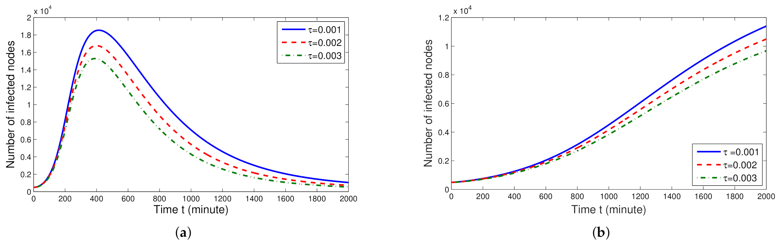
In order to illustrate the reasonableness of the fractional SAIDR model, let us herein investigate the ratio of infection and the ratio of transition between infected and suspended states, which are two substantial variables. Figure 2a,b evince that a larger quantity of nodes will be contaminated more quickly as the infection rate scales up. To put it differently, as for the fractional order and elevates, the worm circulates more swiftly. For this reason, it is possible to say that reducing the infection ratio results in an acceleration of the duration during which the harmful software is wiped out. It follows from Figure 3a,b that the graph hits the lowest point when the graph comes to the topmost more or less simultaneously, approximately at the 400th min, reciprocally involving the three graphs’ highest points. A smaller amount of nodes becomes simultaneously contaminated as a consequence of the escalation in transition ratios to the suspended state from the infected state. The reason is that a smaller number of nodes continue staying in the infected state since a greater amount of nodes are able to shift to the suspended state from the infected state with the escalating ratio.
6. Conclusions
A novel fractional order derivative involving a Mittag–Leffler kernel has recently been introduced by Atangana in cooperation with Baleanu. First and foremost, the AB derivative broadens the scope of the model grounding on [29] so that we can consider the additional implementation of the relevant fractional derivative and monitor the propagation of computer worms in mobile networks more comprehensively. We propound a fractional model which carries the probability of not having any closed form solution since it is nonlinear. Hence, the circumstances providing the existence and uniqueness of the solution regarding this fractional SAIDR model become evident, and the special solution is thus reproduced through the Laplace transform. Lastly, we apply numerical simulations of this model so as to reach efficacy with this novel derivative provided with a fractional order. Additionally, we express the impact that infection ratio has on infected nodes numerically, and on the grounds of the relevant graphics, we conclude that diminishing the ratio of infection speeds up the duration during which the malignant software are eliminated.
Author Contributions
Conceptualization, E.U. and S.U.; methodology, S.U., F.E. and N.Ö.; software, F.E.; validation, E.U., S.U., F.E. and N.Ö.; formal analysis, F.E. and N.Ö.; investigation, E.U., S.U., F.E. and N.Ö.; resources, E.U., S.U., F.E. and N.Ö.; writing—original draft preparation, E.U., S.U., F.E. and N.Ö.; writing—review and editing, E.U., S.U., F.E. and N.Ö.; visualization, S.U. and F.E.; supervision, N.Ö.; project administration, S.U. All authors have read and agreed to the published version of the manuscript.
Funding
This research is supported by Balikesir University Research Grant No. BAP 2020/014.
Data Availability Statement
Not applicable.
Conflicts of Interest
The authors declare no conflict of interest.
References
- Abraham, S.; Smith, I.C. An overview of social engineering malware: Trends, tactics, and implications. Technol. Soc. 2010, 32, 183–196. [Google Scholar] [CrossRef]
- CNCENT/CC, CCKUN-A Mobile Malware Spreading in Social Relationship Networks by SMS. 2013. Available online: https://www.cert.org.cn/publish/main/8/2013/20130924145326642925406/20130924145326642925406_.html (accessed on 10 February 2021).
- Computer World, Android SMS Worm Selfmite Is Back, More Aggressive Than Ever. 2013. Available online: http://www.computerworld.com/article/2824619/android-sms-worm-selfmite-is-back-more-aggressive-than-ever.html (accessed on 10 February 2021).
- CNCENT/CC. The Bulletin about the Outbreak and Response of the xxShenQi Malware. 2014. Available online: https://www.cert.org.cn/publish/main/12/2014/20140803174220396365334/20140803174220396365334_.html (accessed on 10 February 2021).
- Podlubny, I. Fractional Differential Equations: An Introduction to Fractional Derivatives to Methods of Their Solution and Some of Their Applications; Academic Press: San Diego, CA, USA, 1999. [Google Scholar]
- Caputo, M.; Mainardi, F. A new dissipation model based on memory mechanism. Pure Appl. Geophys. 1971, 91, 134–147. [Google Scholar] [CrossRef]
- Caputo, M.; Fabrizio, F. A new definition of fractional derivative without singular kerne. Prog. Fract. Differ. Appl. 2015, 1, 73–85. [Google Scholar]
- Koca, I. Analysis of rubella disease model with non-local and non-singular fractional derivatives. Int. J. Optim. Control Theor. Appl. 2018, 8, 17–25. [Google Scholar] [CrossRef] [Green Version]
- Jajarmi, A.; Baleanu, D. A new fractional analysis on the interaction of HIV with CD4+ T-cells. Chaos Solitons Fractals 2018, 113, 221–229. [Google Scholar] [CrossRef]
- Uçar, S.; Özdemir, N.; Koca, I.; Altun, E. Novel analysis of the fractional glucose insulin regulatory system with non-singular kernel derivative. Eur. Phys. J. Plus 2020, 135, 414. [Google Scholar] [CrossRef]
- Özdemir, N.; Agrawal, O.P.; İskender, B.B.; Karadeniz, D. Fractional optimal control of a 2-dimensional distributed system using eigenfunctions. Nonlinear Dyn. 2009, 55, 251–260. [Google Scholar] [CrossRef]
- Baleanu, D.; Fernandez, A.; Akgül, A. On a fractional operator combining proportional and classical differintegrals. Mathematics 2020, 8, 13. [Google Scholar] [CrossRef] [Green Version]
- Uçar, E.; Özdemir, N.; Altun, E. Fractional order model of immune cells influenced by cancer cells. Math. Model. Nat. 2019, 14, 12. [Google Scholar]
- Evirgen, F.; Özdemir, N. Multistage adomian decomposition method for solving NLP problems over a nonlinear fractional dynamical system. J. Comput. Nonlinear Dyn. 2011, 6. [Google Scholar] [CrossRef]
- Evirgen, F. Conformable Fractional Gradient Based Dynamic System for Constrained Optimization Problem. Acta Phys. Pol. A 2017, 132, 1066–1069. [Google Scholar] [CrossRef]
- Uçar, E.; Özdemir, N. A fractional model of cancer-immune system with Caputo and Caputo–Fabrizio derivatives. Eur. Phys. J. Plus 2021, 136, 1–17. [Google Scholar] [CrossRef] [PubMed]
- Aljoudi, S.; Ahmad, B.; Alsaedi, A. Existence and uniqueness results for a coupled system of Caputo-Hadamard fractional differential equations with nonlocal Hadamard type integral boundary conditions. Fractal Fract. 2020, 4, 15. [Google Scholar] [CrossRef] [Green Version]
- Baleanu, D.; Hakimeh, M.; Shahram, R. A fractional differential equation model for the COVID-19 transmission by using the Caputo–Fabrizio derivative. Adv. Differ. Eq. 2020, 2020, 299. [Google Scholar] [CrossRef] [PubMed]
- Aliyu, A.I.; Inc, M.; Yusuf, A.; Baleanu, D. A fractional model of vertical transmission and cure of vector-borne diseases pertaining to the Atangana–Baleanu fractional derivatives. Chaos Solitons Fractals 2018, 116, 268–277. [Google Scholar] [CrossRef]
- Uçar, S. Analysis of a basic SEIRA model with Atangana-Baleanu derivative. AIMS Math. 2020, 5, 1411–1424. [Google Scholar] [CrossRef]
- Kumar, D.; Singh, J. New aspects of fractional epidemiological model for computer viruses with Mittag–Leffler law. In Mathematical Modelling in Health, Social and Applied Sciences; Dutta, H., Ed.; Springer: Singapore, 2020; pp. 283–301. [Google Scholar]
- Atangana, A.; Baleanu, D. New fractional derivatives with nonlocal and non-singular kernel: Theory and application to heat transfer model. Therm. Sci. 2016, 20, 763–769. [Google Scholar] [CrossRef] [Green Version]
- Fernandez, A.; Baleanu, D.; Srivastava, H.M. Series representations for fractional-calculus operators involving generalised Mittag-Leffler functions. Commun. Nonlinear Sci. Numer. 2019, 67, 517–527. [Google Scholar] [CrossRef] [Green Version]
- Baleanu, D.; Jajarmi, A.; Hajipour, M. On the nonlinear dynamical systems within the generalized fractional derivatives with Mittag-Leffler kernel. Nonlinear Dyn. 2018, 94, 397–414. [Google Scholar] [CrossRef]
- Qureshi, S.; Yusuf, A.; Shaikh, A.A.; Inc, M.; Baleanu, D. Fractional modeling of blood ethanol concentration system with real data application. Chaos 2019, 29, 131–143. [Google Scholar] [CrossRef]
- Uçar, S.; Uçar, E.; Özdemir, N.; Hammouch, Z. Mathematical analysis and numerical simulation for a smoking model with Atangana-Baleanu derivative. Chaos Solitons Fractals 2019, 118, 300–306. [Google Scholar] [CrossRef]
- Yavuz, M.; Özdemir, N.; Başkonuş, H.M. Solutions of partial differential equations using the fractional operator involving Mittag-Leffler kernel. Eur. Phys. J. Plus 2018, 133, 1–11. [Google Scholar] [CrossRef]
- Fernandez, A.; Husain, I. Modified Mittag-Leffler functions with applications in complex formulae for fractional calculus. Fractal Fract. 2020, 4, 15. [Google Scholar] [CrossRef]
- Xiao, X.; Fu, P.; Hu, G.; Sangiah, A.K.; Zheng, H.; Jiang, Y. SAIDR: A new dynamic model for SMS-based worm propagation in mobile networks. IEEE Access 2017, 5, 9935–9943. [Google Scholar] [CrossRef]
- Baleanu, D.; Fernandez, A. On some new properties of fractional derivatives with Mittag-Leffler kernel. Commun. Nonlinear Sci. Numer. Simul. 2018, 59, 444–462. [Google Scholar] [CrossRef] [Green Version]
- Gómez-Aguilar, J.F.; Rosales-García, J.J.; Bernal-Alvarado, J.J. Fractional mechanical oscillators. Rev. Mex. FíSica 2012, 58, 348–352. [Google Scholar]
- Qing, Y.; Rhoades, B.E. T-stability of Picard iteration in metric spaces. Fixed Point Theory Appl. 2008, 2008. [Google Scholar] [CrossRef] [Green Version]
- Mekkaoui, T.; Atangana, A. New numerical approximation of fractional derivative with non-local and non-singular kernel: Application to chaotic models. Eur. Phys. J. Plus 2017, 132, 1–16. [Google Scholar]
Figure 1.
Numerical simulation of Equation (6) for (a) ; (b) ; (c) ; and (d) .
Figure 1.
Numerical simulation of Equation (6) for (a) ; (b) ; (c) ; and (d) .

Figure 2.
Effect of on the infected nodes for the fractional order (a) and (b) , respectively.
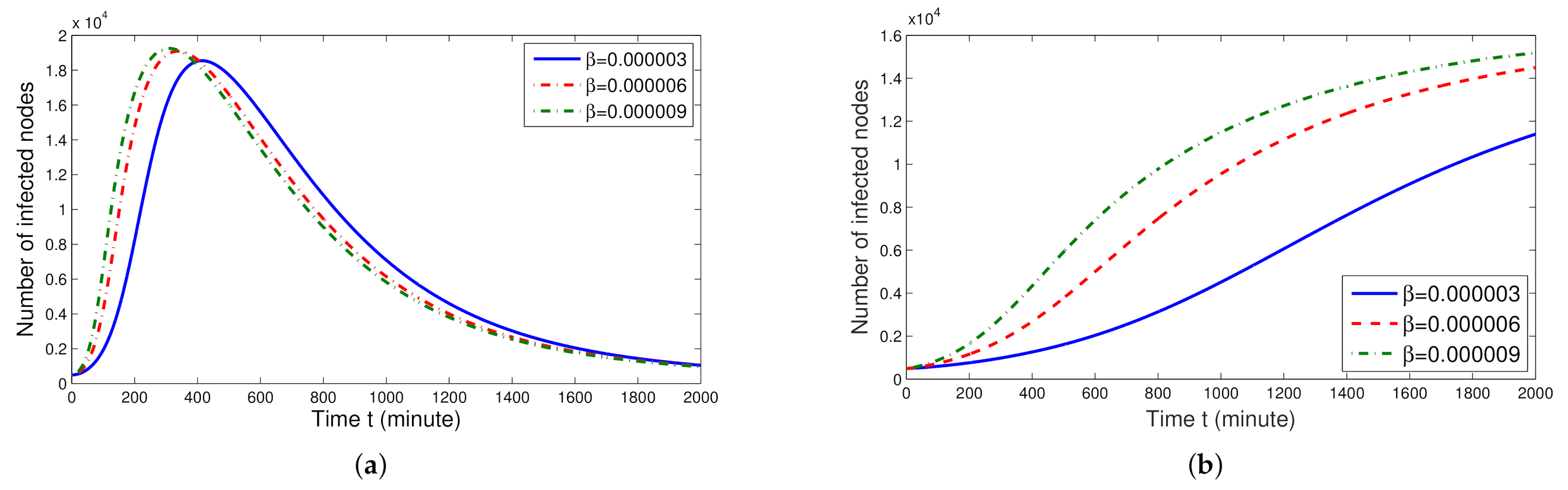
Figure 3.
Relation between and infected nodes for the fractional order (a) and (b) , respectively.
Publisher’s Note: MDPI stays neutral with regard to jurisdictional claims in published maps and institutional affiliations. |
© 2021 by the authors. Licensee MDPI, Basel, Switzerland. This article is an open access article distributed under the terms and conditions of the Creative Commons Attribution (CC BY) license (https://creativecommons.org/licenses/by/4.0/).
Share and Cite
MDPI and ACS Style
Uçar, E.; Uçar, S.; Evirgen, F.; Özdemir, N. A Fractional SAIDR Model in the Frame of Atangana–Baleanu Derivative. Fractal Fract. 2021, 5, 32. https://doi.org/10.3390/fractalfract5020032
AMA Style
Uçar E, Uçar S, Evirgen F, Özdemir N. A Fractional SAIDR Model in the Frame of Atangana–Baleanu Derivative. Fractal and Fractional. 2021; 5(2):32. https://doi.org/10.3390/fractalfract5020032
Chicago/Turabian StyleUçar, Esmehan, Sümeyra Uçar, Fırat Evirgen, and Necati Özdemir. 2021. "A Fractional SAIDR Model in the Frame of Atangana–Baleanu Derivative" Fractal and Fractional 5, no. 2: 32. https://doi.org/10.3390/fractalfract5020032