Article

An Extended Dissipative Analysis of Fractional-Order Fuzzy Networked Control Systems

by
Rajarathinam Vadivel
1,
Porpattama Hammachukiattikul
1,
Seralan Vinoth
2,
Kantapon Chaisena
1 and
Nallappan Gunasekaran
3,*
1
Department of Mathematics, Faculty of Science and Technology, Phuket Rajabhat University, Phuket 83000, Thailand
2
Centre for Nonlinear Systems, Chennai Institute of Technology, Chennai 600 069, Tamilnadu, India
3
Computational Intelligence Laboratory, Toyota Technological Institute, Nagoya 468-8511, Japan
*
Author to whom correspondence should be addressed.
Fractal Fract. 2022, 6(10), 591; https://doi.org/10.3390/fractalfract6100591
Submission received: 16 August 2022 / Revised: 22 September 2022 / Accepted: 5 October 2022 / Published: 13 October 2022

Abstract

:
This study presents an extended dissipative analysis of fractional order fuzzy networked control system with uncertain parameters. First, we designed the network-based fuzzy controller for the considered model. Second, a novel Lyapunov-Krasovskii functional (LKF) approach, inequality techniques, and some sufficient conditions are established, which make the proposed system quadratically stable under the extended dissipative criteria. Subsequently, the resultant conditions are expressed with respect to linear matrix inequalities (LMIs). Meanwhile, the corresponding controller gains are designed under the larger sampling interval. Finally, two numerical examples are presented to illustrate the viability of the obtained criteria.

1. Introduction

In recent years, fractional order (FO) differential equations have received considerable attention due to their extensive applications in real life. By exploiting the theory and measures of dynamics, qualitative and quantitative discussions of the behaviour of the fractional order system are implemented. It is important to realize that fractional order differential equation applied widely in nature [1,2,3]. The dynamics of the fractional-order model have always been concerned. Researching the strange behavior of dynamical systems in physics, biology, chemistry, electrical, and chaotic systems makes use of fractional-order systems [4,5]. The most effective methods for describing these cases are the Mittag-Leffler functions. No significant geometrical interpretation, such as the trend of functions or their convexity, is related to the idea of fractional calculus. Due to their extensive memory, fractional order differential equations can store the complete function’s information. Many researchers are currently conducting research that is ahead of this field, and they have produced several impressive results, both theoretically and numerically. In [6], the authors have investigated synchronization control for the Riemann-Liouville fractional competitive network systems. The problem of optimal control for the nonlinear fractional-order systems with multiple time-varying delays has been studied in [7]. Stability analysis of neutral-type fractional order systems with nonlinear perturbations and input saturation has been researched in [8].
Takagi-Sugeno (T-S) fuzzy models aim for the expression of nonlinear dynamics by linear models with fuzzy membership functions. We know that T-S fuzzy systems have been successfully used to articulate practical systems since they are straightforward and convenient to use when faced with complex nonlinearity [9,10]. As an outcome, numerous results regarding T-S fuzzy model stability and stabilization issues have been published. However, due to the difficulty of modern systems, several practical models, including viscoelastic and biological systems, cannot be demonstrated in integer order [11,12]. In contrast to integer-order derivatives, fractional derivatives have unique characteristics like inheritance, memory, nonlocality, and others. Control of fractional-order systems, particularly control of non-linear fractional-order systems, has generally been one of the rapidly growing research fields. To examine the stability and stabilization of fractional-order fuzzy systems, different techniques were developed [13,14,15,16]. In specific, fractional-order systems can be constructed to the T-S fuzzy model. For instance, the authors in [13] investigated the finite-time stability of fuzzy cellular neural networks with fractional orders and time delays.
Dynamical control of fractional-order differential systems including stabilisation is a prevalent topic currently and many interesting results have been obtained based on fault-tolerant control [16], output feedback control [17], observer-based control [3], containment control [18], and guaranteed cost control [19]. It has been noted that the state feedback controller is typically unreliable due to the fact that it demands complete state information and drives up the cost of implementation and the difficulty of connecting control parameters. Control systems with different components such as sensors, controllers, and actuators connected via communication networks are known as networked control systems (NCSs) [20,21]. Compared with standard control systems, NCSs have been increasing research interests due to their advantages in low cost, reduced weight, high reliability, stability analysis, and wide applications in science and engineering [22,23]. Consequently, it is crucial to use a sophisticated control approach known as a decentralized static output feedback controller, which is more successful in real control schemes. There have been numerous studies on the modeling, stability analysis, and control design of NCSs [20,21,22,23]. Several control algorithms have been extensively investigated by researchers to address the stability and stabilisation analysis of fractional-order NCSs with or without using the Lyapunov functional theory. Furthermore, the concept of extended dissipative plays a very important role in performance analysis [24], which unifies H performance, L 2 L performance, passivity performance and ( Q S R ) -dissipativity performance together. It has received a great deal of attention since it provides an effective way for system performance analysis [25,26,27]. As a result, this research aims to examine the extended dissipative performance of fuzzy fractional order networked control system (FFONCS). The difficulties of delayed fractional-order NCSs with extended dissipative approaches were not completely addressed and continue to be difficult in comparison to previous work. To keep the stability and stabilization efficiencies of the FFONCS, it is crucial to take into account the effects of time-varying network delays and the extended dissipative approach in this work.
Encouraged by the above analysis, we shall present the theoretical analysis of the delayed FFONCS with extended dissipative analysis. The objectives of this paper are as follows:
  • In this paper, the extended dissipativity and control synthesis is concerned for FFONCSs with time-varying delay. Up to now, there has been no result on these problems since solving their needs not only to deal with the extended dissipative performance for the underlying FFONCS but also to handle the Lyapunov-Krasovskii functional (LKF) theory.
  • In this study, NCSs with time-varying delays, which takes place in the sensor-to-controller and controller-to-actuator channels are investigated.
  • For the stabilization analysis of the proposed system model, novel LKF based on fractional order derivative is constructed, which can fully take more information about the sampling interval, using novel integral inequality and some new adequate conditions to ensure the asymptotic stability of FFONCS which are derived with respect to linear matrix inequalities (LMI).
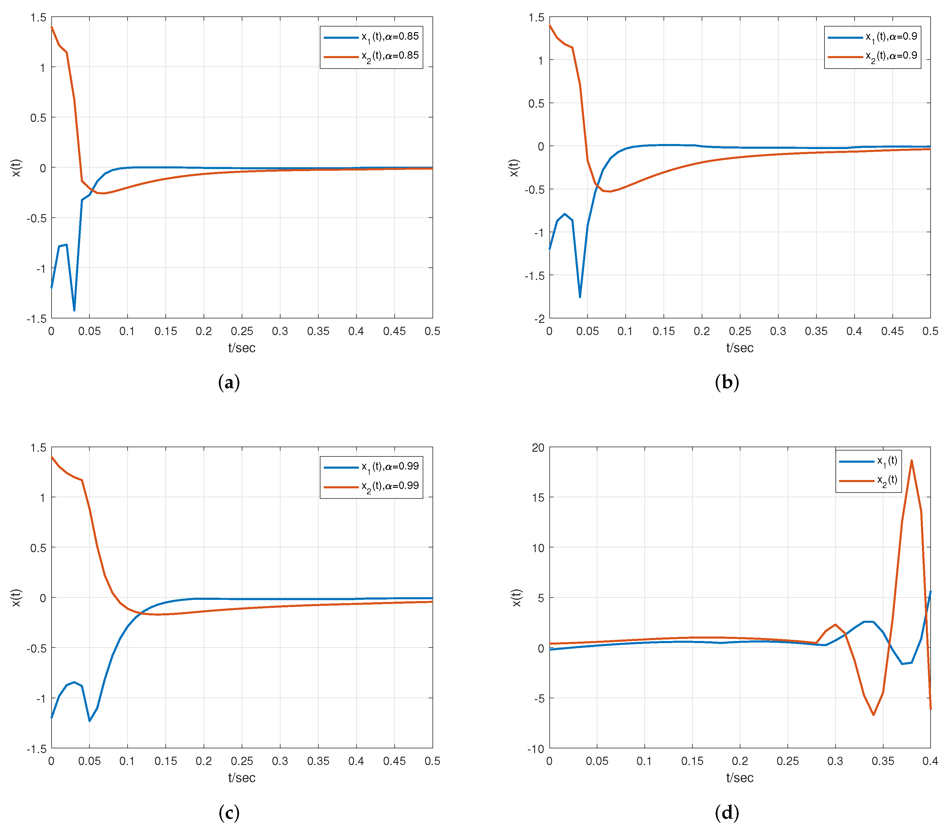
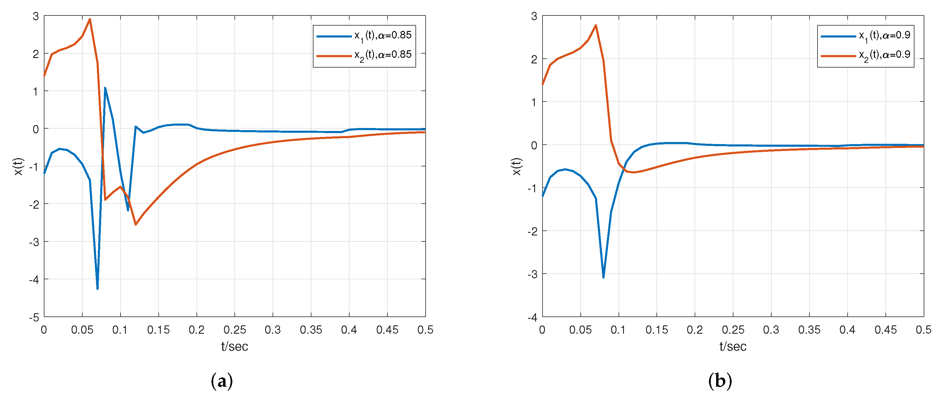
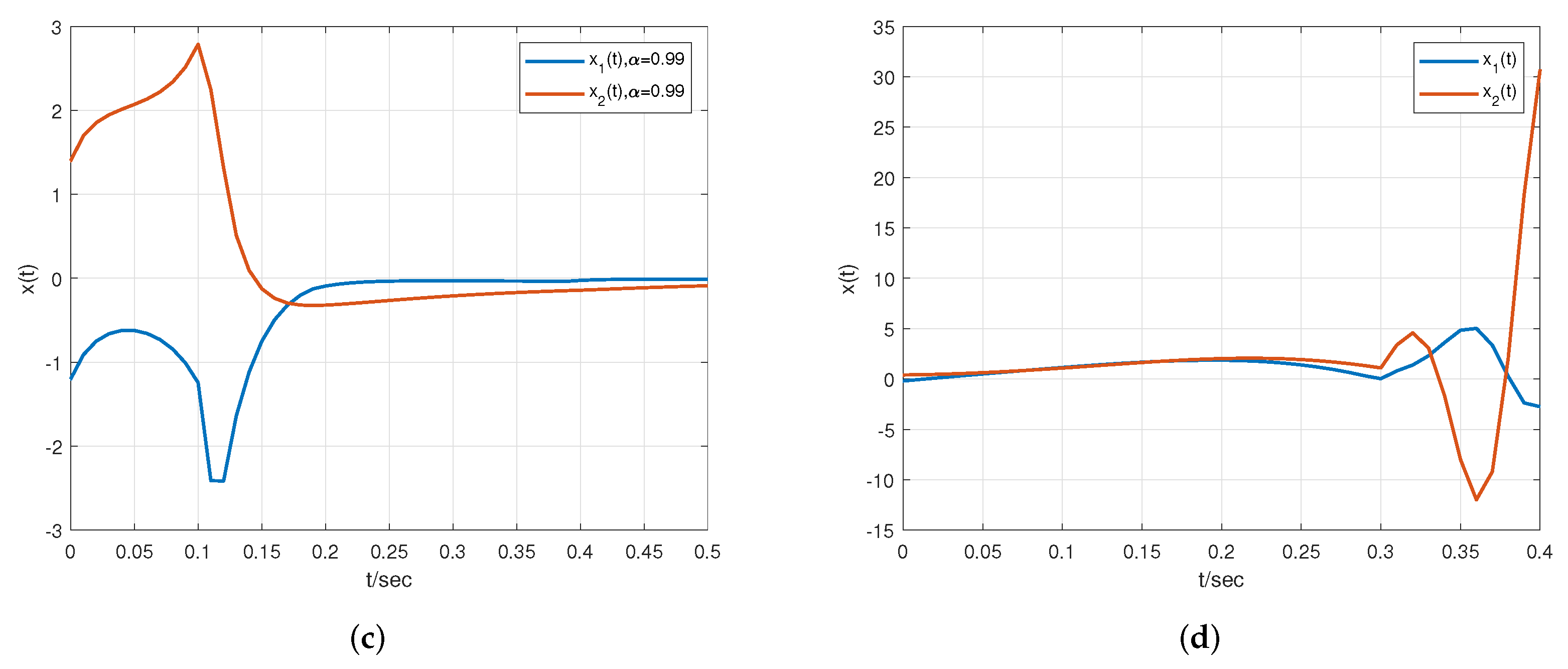
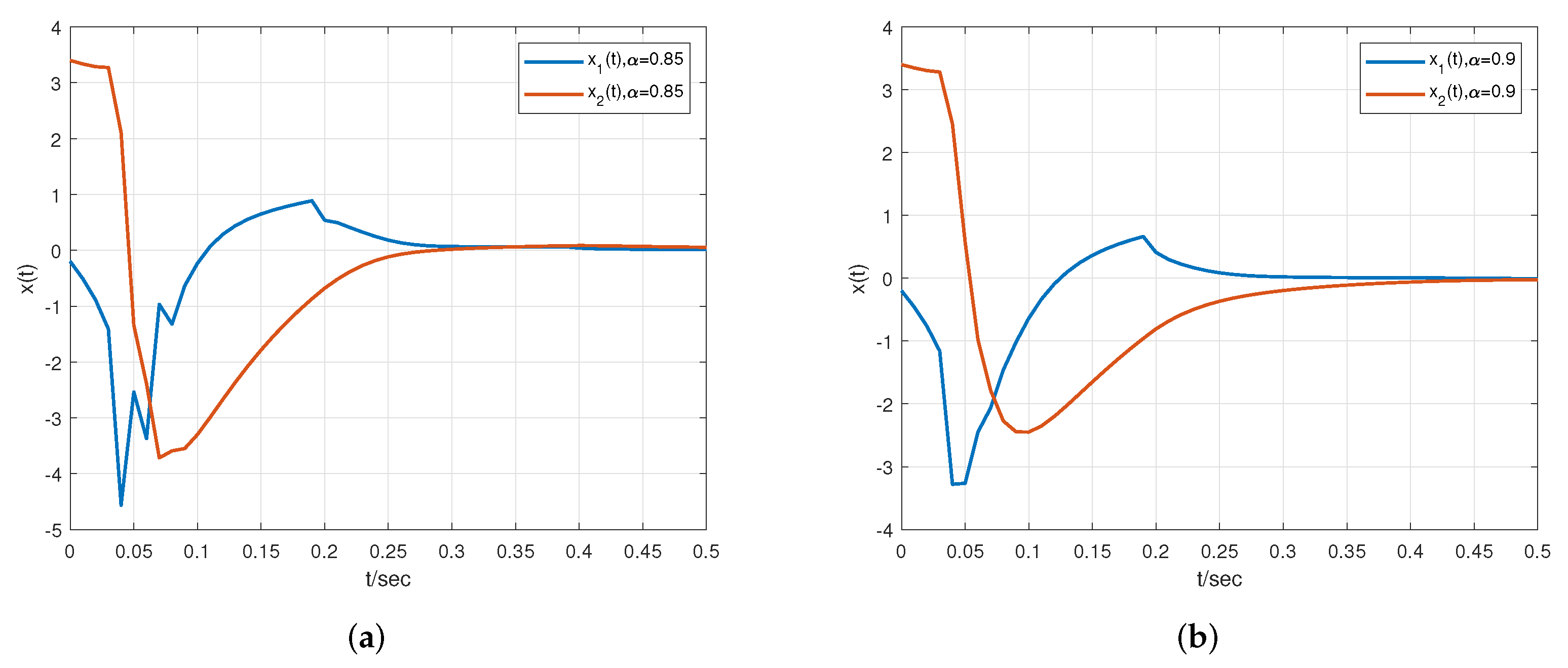
  • Finally, numerical simulations are proposed to illustrate the effectiveness and applicability of the suggested theories.
Notation: For any matrix X R n × m , the notation X > 0 or X 0 indicates that X is positive definite or positive semidefinite, Q 1 and Q T are noted as inverses and transposes of Q, respectively. I stands for identity matrix with the corresponding dimensions. * is used to indicate the symmetric terms in the symmetric matrix. R n and R n × m denote the n dimensional Euclidean space and the set of n × m real matrices.

2. Problem Formulation and Preliminaries

Now, we consider the nonlinear fractional-order systems with time-varying delay, which is of the form
0 C D t α x ( t ) = f ( x ( t ) , x ( t τ ( t ) ) , u ( t ) , w ( t ) ) , x ( s ) = φ ( s ) , s [ τ , 0 ] , α ( 0 , 1 ) ,
where α ( 0 , 1 ) , x ( t ) R n is the pseudo-state vector, u ( t ) R m is the control input, w ( t ) is the external input, and τ ( t ) is a time-varying delay which needs to satisfy 0 τ ( t ) τ and τ ˙ ( t ) μ with τ > 0 , μ > 0 , and φ ( s ) is a continuous vector-valued initial function on the [ τ , 0 ] . Nonlinear delayed fractional-order system (1) can be modeled by the respective T-S fuzzy delay fractional-order uncertain system with r rules.
Rule i: If θ 1 ( t ) is M i 1 , θ 2 ( t ) is M i 2 , , θ p ( t ) is M i p , then
C D α x ( t ) = A i ( t ) x ( t ) + A d i ( t ) x ( t τ ( t ) ) + B i ( t ) u ( t ) + w ( t ) , t 0 , x ( s ) = φ ( s ) , s [ τ , 0 ] ,
where θ 1 ( t ) , θ 2 ( t ) , , θ p ( t ) are the known premise variables, and M i l ( i = 1 , 2 , , r , l = 1 , 2 , , p ) are fuzzy sets, A i ( t ) = A i + Δ A i , A d i ( t ) = A d i + Δ A d i , and B i ( t ) = B i + Δ B i are known real constant matrices with suitable dimensions, and Δ A i , Δ A d i , and Δ B i are unknown matrices with the real values representing uncertainties of time-varying parameters and are considered to be in the form
[ Δ A i Δ A d i Δ B i ] = Y i F i ( t ) [ ξ 1 i ξ 2 i ξ 3 i ] ,
where Y i , ξ 1 i , ξ 2 i and ξ 3 i are known real constant matrices and F i ( t ) is the unknown time-varying matrix function holds
F i T ( t ) F i ( t ) I .
The resultant fuzzy model can be defined as follows
C D α x ( t ) = i = 1 r h i ( θ ( t ) ) { A i ( t ) x ( t ) + A d i ( t ) x ( t τ ( t ) ) + B i ( t ) u ( t ) + w ( t ) } , x ( s ) = φ ( s ) , s [ τ , 0 ] , t 0 ,
where fuzzy weighting functions are written as
h i ( θ ( t ) ) = l = 1 p M i l ( θ ( t ) ) i = 1 r l = 1 p M i l ( θ ( t ) ) , i = 1 , 2 , , r .
The term M i l ( · ) is the grade of membership of M i l . We consider that
l = 1 p M i l ( θ ( t ) ) > 0 , i = 1 r l = 1 p M i l ( θ ( t ) ) > 0 , i = 1 , 2 , , r ,
for any θ ( t ) , then we get
i = 1 r h i ( θ ( t ) ) = 1 , h i ( θ ( t ) ) 0 , i = 1 , 2 , , r .
Furthermore, the output system of (5) is written by
y ( t ) = x ( t ) + x ( t τ ( t ) ) .
Next, we consider that the network will be used to control the system (5). The network control structure for a fractional order system with induced delays is shown in Figure 1. The building of a state feedback controller to stabilize the system is the emphasis of this section. Moreover, it is expected that the states of the system (5) are mostly not attainable for measurement; this is why we accomplish an output feedback control. For each subsystem in (5), the control scheme type parallel distributed compensation (PDC) will be considered. The input signal in system (5) for t k t t k + 1 comes from zero-order-hold (ZOH) as follows
u ( t ) = i = 1 r h i ( θ ( t k ) ) K i x ( t k τ k i ) .
A communication delay between sensors and controllers τ s c i , a communication delay between the controller and actuators τ c a i , and the computational time on the controller τ c can all be incorporated into the delay from the controller to the actuator in NCSs. A reasonable assumption on τ k i can be expressed as
0 < τ m i τ k i τ M i .
Packet dropouts are network-induced effects that might occur as a result of a connection breakdown. When this is done on purpose, the most recent information is presented in order to reduce congestion. Despite the fact that most network protocols have transmission-retry capabilities, they only can re-transmit for a certain amount of time. The packets are dropped once this time has passed. Feedback controllers can often endure a particular degree of packet loss. Consecutive packet losses, on the other hand, have a negative impact on overall performance.
t k + 1 t k = λ i T e + max i { τ ( k + 1 ) i } min i { τ k i } ,
where T e is the sample period, t k is the sampling instant, and λ i is the maximum number of packet dropouts during the update periods. Moreover, by defining h ( t ) = t t k + τ k , t k t t k + 1 , we have
τ k h ( t ) λ T e + max { τ ( k + 1 ) } .
Then, we get h ^ 1 h ( t ) h ^ 2 , h ˙ ( t ) μ 1 and h ^ 1 = τ m and h ^ 2 = λ T e + max { τ M } . Then, the system (5) can be given by:
C D α x ( t ) = i = 1 r h i θ ( t ) j = 1 r h j θ ( t k ) { A i ( t ) x ( t ) + A d i ( t ) x ( t τ ( t ) ) + B i ( t ) K j x ( t h ( t ) ) + w ( t ) } , x ( s ) = φ ( s ) , s [ τ , 0 ] , t 0 .
Assumption 1.
Each subsystem’s real input u i ( t ) is a piecewise constant function represented via a ZOH. Since the sample period of a sensor is determined for the design of control algorithms, it is fair to assume that the sensor is clock-driven. When compared to an actuator, which modifies its output to the controlled plant only when given a new control signal, an actuator is event-driven.
Assumption 2.
Matrices χ 1 , χ 2 , χ 3 , and χ 4 satisfy the following conditions:
1. χ 1 = χ 1 T 0 , χ 3 = χ 3 T > 0 , χ 4 = χ 4 T 0 .
2. | | χ 1 | | + | | χ 2 | | . | | χ 4 | | = 0 .
The following Lemmas and Definitions are used in the main results.
Definition 1
([24]). For input matrices χ 1 , χ 2 , χ 3 , and χ 4 fulfilling the assumption (A3), the system (10) with (6) is termed as extended dissipative, and a scalar δ > 0 for which the subsequent relation holds for all t f 0 .
0 t f J ( t ) d t sup y T ( t ) χ 4 y ( t ) + δ , 0 t t f ,
where J ( t ) = y T ( t ) χ 1 y ( t ) + 2 y T ( t ) χ 2 w ( t ) + w T ( t ) χ 3 w ( t ) .
Definition 2
([24]). Assume that w ( t ) = 0 . The system (10) is quadratically stable if a scalar v > 0 exists for which the derivative of the Lyapunov function concerning time t fulfills V ˙ ( t ) v | x ( t ) | 2 .
Definition 3
([28]). The Riemann-Liouville fractional integral is represented as (12).
t 0 I t α f ( t ) = 1 Γ ( α ) t 0 t ( t τ ) α 1 f ( τ ) d τ , α R + ,
where Γ ( · ) is defined as the gamma function.
Definition 4
([28]). The Caputo fractional order derivative (CFOD) is introduced as.
t 0 C D t α f ( t ) = 1 Γ ( n α ) × t 0 t ( t τ ) n α 1 f n ( τ ) d τ ,
where n 1 α n .
Lemma 1
([29]). For a function F ( t ) = α ( t ) β ( t ) f ( s , t ) d s , where α 4 ( t ) , α 2 ( t ) are differentiable, f ( s , t ) is continuous concerning s and differentiable in relation to t, equality (14) holds.
d F ( t ) d t = β ˙ ( t ) f ( β ( t ) , t ) α ˙ ( t ) f ( α ( t ) , t ) + α ( t ) β ( t ) f ( s , t ) t d s .
Lemma 2
([30]). Let M R n × n be a positive definite constant matrix and Υ ˜ ˜ > 0 is a scalar, if a vector function ω ˜ ˜ : [ 0 , Υ ˜ ˜ ] R n exists such that the integrals 0 Υ ˜ ˜ ω ˜ ˜ T ( s ) M ω ˜ ˜ ( s ) d s and 0 Υ ˜ ˜ ω ˜ ˜ T ( s ) d s are well defined, then inequality (15) holds.
Υ ˜ ˜ 0 Υ ˜ ˜ ω ˜ ˜ T ( s ) M ω ˜ ˜ ( s ) d s 0 Υ ˜ ˜ ω ˜ ˜ T ( s ) d s M 0 Υ ˜ ˜ ω ˜ ˜ ( s ) d s .
Lemma 3
([31]). Assume that x ( t ) R n is a vector of differentiable functions. Inequality (16) holds for any time instant t > t 0 .
1 2 t 0 C D t α x T ( t ) P x ( t ) x T ( t ) P t 0 C D t α x ( t ) , α ( 0 , 1 ) ,
where P R n × n is a constant, square, and positive definite matrix.
Remark 1.
Based on the Definition 1, we can provide the subsequent analysis
(1) L 2 L performance: χ 1 = 0 , χ 2 = 0 , χ 3 = γ ˜ 2 I , χ 4 = I , and δ = 0 .
(2) H performance: χ 1 = I , χ 2 = 0 , χ 3 = γ ˜ 2 I , χ 4 = 0 , and δ = 0 .
(3) Passivity performance: χ 1 = 0 , χ 2 = I , χ 3 = γ ˜ I , χ 4 = 0 , and δ = 0 .
(4) Mixed H and Passivity performance: χ 1 = γ ˜ 1 α ˜ I , χ 2 = ( 1 α ˜ ) I , χ 3 = γ ˜ I , χ 4 = 0 with α ˜ = 0.5 .
(5) ( Q S R ) Dissipativity performance: χ 1 = Q , χ 2 = S , χ 3 = R γ ˜ I , and χ 4 = 0 .

3. Main Results

In this section, an extended dissipativity investigation for delayed FFONCS (10) in the form of LMIs will be established for all nonzero w ( t ) and without uncertain parameters in the following Theorem 1.
Theorem 1.
For the given positive scalars τ , μ , μ 1 , h ^ 1 , h ^ 2 , given control gains K j , and 0 < ϵ < 1 , matrices χ 1 , χ 2 , χ 3 , and χ 4 satisfying the Assumption 2, FFONCS (10) is quadratically stable and extended dissipative, such that there exist symmetric matrices P > 0 , Q > 0 , R > 0 , W > 0 , W 1 > 0 , W 2 > 0 , and T > 0 , any matrix of compatible dimension H 1 , satisfying the subsequent LMIs:
Ξ i j = Ξ 11 Ξ 12 * Ξ 22 < 0 ,
Π = ε P χ 4 χ 4 * ( 1 ε ) P χ 4 > 0 ,
where
Ξ 11 = Ξ ^ 11 P A d i χ 1 A T H 1 T 0 * ( 1 μ ) Q χ 1 A d T H 1 T 0 * * Ξ ^ 33 0 * * * R , Ξ 22 = W 1 0 0 0 0 * ( 1 μ ) W 2 0 0 0 * * W 0 0 * * * T 0 * * * * χ 3 , Ξ 12 = [ Ξ a a T Ξ b b T Ξ c c T Ξ d d T Ξ e e T ] , Ξ a a = Ξ d d = [ 0 0 0 0 ] , Ξ b b = [ ( P B i K j ) T 0 ( H 1 B i K j ) T 0 ] , Ξ c c = [ 0 0 0 0 ] , Ξ ^ 11 = 2 P A i + Q + W + W 1 + W 2 χ 1 , Ξ ^ 33 = τ 2 R + h ^ 2 2 T 2 H 1 , Ξ e e = [ χ 2 χ 2 0 0 ] .
Furthermore, from Definition 1 the scalar δ assigned as δ = V ( 0 ) | | P | | sup max ( τ , h ^ 2 ) s 0 | ϕ ( s ) | 2 .
Proof. 
Construct the functional candidate with LKF:
V ( t ) = c = 1 4 V c ( t ) ,
where
V 1 ( t ) = x T ( t ) P x ( t ) , V 2 ( t ) = t τ ( t ) t x T ( s ) Q x ( s ) d s + τ τ 0 t + θ t C D α x T ( s ) R C D α x ( s ) d s d θ , V 3 ( t ) = t h ^ 2 t x T ( s ) W x ( s ) d s + h ^ 2 h ^ 2 0 t + θ t C D α x T ( s ) T C D α x ( s ) d s d θ , V 4 ( t ) = t h ^ 1 t x T ( s ) W 1 x ( s ) d s + t h ( t ) t x T ( s ) W 2 x ( s ) d s .
By using Definitions 3 and 4, the derivatives of V l ( t ) , l = 1 , 2 , , 4 in connection to t as well as the trajectories of system (10), we get
V ˙ ( t ) V ˙ 1 ( t ) + V ˙ 2 ( t ) + V ˙ 3 ( t ) + V ˙ 4 ( t ) , = x T ( t ) P C D t α x ( t ) + x T ( t ) Q x ( t ) ( 1 μ ) x T ( t τ ( t ) ) Q x ( t τ ( t ) ) + τ 2 C D α x T ( t ) R C D α x ( t ) τ t τ t C D α x T ( s ) R C D α x ( s ) d s + x T ( t ) W x ( t ) x T ( t h ^ 2 ) W x ( t h ^ 2 ) + h ^ 2 2 t o C D t α x T ( t ) T C D α x ( t ) h ^ 2 t h ^ 2 t C D α x T ( s ) T C D α x ( s ) d s + x T ( t ) W 1 x ( t ) x T ( t h ^ 1 ) W 1 x ( t h ^ 1 ) + x T ( t ) W 2 x ( t ) ( 1 μ 1 ) x T ( t h ( t ) ) W 2 x ( t h ( t ) ) ,
with Lemma 2 & 3, we get
2 x T ( t ) P A i x ( t ) + 2 x T ( t ) P A d i x ( t τ ( t ) ) + 2 x T ( t ) P B i K j x ( t h ( t ) ) + x T ( t ) Q x ( t ) ( 1 μ ) x T ( t τ ( t ) ) Q x ( t τ ( t ) ) + τ 2 t 0 C D t α x T ( t ) R C D α x ( t ) x T ( t h ^ 2 ) W x ( t h ^ 2 ) t τ t C D α x T ( s ) d s R t τ t C D α x ( s ) d s + x T ( t ) W x ( t ) + h ^ 2 2 C D α x T ( t ) T C D α x ( t ) t h ^ 2 t C D α x T ( s ) d s T t h ^ 2 t C D α x ( s ) d s + x T ( t ) W 1 x ( t ) x T ( t h ^ 1 ) W 1 x ( t h ^ 1 ) + x T ( t ) W 2 x ( t ) ( 1 μ 1 ) x T ( t h ( t ) ) W 2 x ( t h ( t ) ) .
The resulting equation holds for any compatible dimension matrix H 1 :
0 = 2 [ C D α x T ( t ) ] H 1 [ C D α x ( t ) + A i x ( t ) + A d i x ( t τ ( t ) ) + B i K j x ( t h ( t ) ) + w ( t ) ] .
Now, consolidating (19) and (20), we conclude that
V ˙ ( t ) J ( t ) ξ T ( t ) Ξ i j ξ ( t ) ,
where Ξ i j is defined in (17) and
ξ T ( t ) = [ x T ( t ) x T ( t τ ( t ) ) C D α x T ( t ) t τ t C D α x T ( s ) d s x T ( t h ^ 1 ) x T ( t h ( t ) ) x T ( t h ^ 2 ) t h ^ 2 t C D α x T ( s ) d s w T ( t ) ] .
Since Ξ < 0 and the relation to scalar ν > 0 , consequently Ξ ν I , then
V ˙ ( x ( t ) ) J ( t ) ν | Γ ( t ) | 2 ν | x ( t ) | 2 ,
i . e . , V ˙ ( x ( t ) ) J ( t ) ν | x ( t ) | 2 .
Taking into account w ( t ) = 0 yields
J ( t ) = y T ( t ) χ 1 y ( t ) .
Observing χ 1 0 with respect to Assumption 2 produces V ˙ ( t ) ν | x ( t ) | 2 .
We conclude that (10) is quadratically stable. Now, we analyze the system’s extended dissipativity condition. It is clear that
V ˙ ( x ( t ) ) J ( t ) 0 .
Integrating (22) with limits 0 to t on both sides, yields that
0 t J ( t ) d t V ( x ( t ) ) V ( 0 ) x T ( t ) P x ( t ) + δ .
The aforementioned scenarios are required to manifest the validity of (11). As a result, we investigate two circumstances: χ 4 = 0 and χ 4 0 . To proceed, if χ 4 = 0 and t f 0 (23) indicates that
0 t f J ( t ) d t x T ( t f ) P x ( t f ) + δ δ .
which demonstrates that Theorem 1 is true. Assuming χ 4 0 , as stated in Assumption 2, we may deduce that χ 1 = 0 , χ 2 = 0 , and χ 3 > 0 . If t f t 0 , yields that
0 t f J ( t ) d t 0 t J ( t ) d t x T ( t ) P x ( t ) + δ .
Also, t > τ ( t ) , we get 0 < t τ ( t ) t f .
Therefore,
0 t f J ( t ) d t x T ( t τ ( t ) ) P x ( t τ ( t ) ) + δ .
In addition to, if t τ ( t ) , then τ t τ ( t ) 0 , it is possible to confirm that
δ + x T ( t τ ( t ) ) P x ( t τ ( t ) ) δ + P | x ( t τ ( t ) ) | 2 δ + | | P | | sup | ϕ ( ν ) | 2 , V ( 0 ) 0 t f J ( t ) d t .
The above equation shows that (26) achieves for every t f t 0 . Consequently, we know from above inequalities (25) and (26), and belongs to scalar 0 < ε < 1 such that
0 t f J ( t ) d t δ + ε x T ( t ) P x ( t ) + ( 1 ε ) x T ( t τ ( t ) ) P x ( t τ ( t ) ) .
Observing the concept that
y T ( t ) χ 4 y ( t ) = x ( t ) x ( t τ ( t ) ) T Π x ( t ) x ( t τ ( t ) ) + ε x T ( t ) P x ( t ) + ( 1 ε ) x T ( t τ ( t ) ) P x ( t τ ( t ) ) ,
for Π > 0 , then
y T ( t ) χ 4 y ( t ) ε x T ( t ) P x ( t ) + ( 1 ε ) x T ( t τ ( t ) ) P x ( t τ ( t ) ) .
This demonstrates that for every t 0 , t f 0 , with t f t ,
0 t f J ( t ) d t y T ( t ) χ 4 y ( t ) + δ .
As a result, (11) holds for any t f 0 . As per the foregoing analysis, the system studied in (6) is extended dissipative for χ 4 = 0 and χ 4 0 concerning Definition 1, which completes the proof. □
Now, the following Theorem 1 extends the criterion of Theorem 2 to obtain a extended dissipative analysis for uncertain system (10) (i.e., Δ A i Δ A d i Δ B i 0 ) .
Theorem 2.
For given positive scalars τ , μ , μ 1 , h ^ 1 , h ^ 2 , K j , and 0 < ϵ < 1 , matrices χ 1 , χ 2 , χ 3 , and χ 4 acceptable Assumption 2, robust FFONCS (10) is quadratically stable and extended dissipative, such that there exist matrices P > 0 , Q > 0 , R > 0 , W > 0 , W 1 > 0 , W 2 > 0 , T > 0 , any compatible dimensioned matrix H 1 , scalar ϱ > 0 , and the following LMIs hold:
Ξ ^ i j = Ξ 11 Ξ 12 Y ¯ ϱ λ T * Ξ 22 0 0 * * ϱ I 0 * * * ϱ I < 0 ,
Π = ε P χ 4 χ 4 * ( 1 ε ) P χ 4 > 0 ,
where
Ξ 11 = Ξ ^ 11 P A d i χ 1 A i T H 1 T 0 * ( 1 μ ) Q χ 1 A d i T H 1 T 0 * * Ξ ^ 33 0 * * * R , Ξ 22 = W 1 0 0 0 0 * ( 1 μ ) W 2 0 0 0 * * W 0 0 * * * T 0 * * * * χ 3 , Ξ 12 = [ Ξ a a T Ξ b b T Ξ c c T Ξ d d T Ξ e e T ] , Ξ a a = Ξ d d = [ 0 0 0 0 ] , Ξ b b = [ ( P B i K j ) T 0 ( H 1 B i K j ) T 0 ] , Ξ c c = [ 0 0 0 0 ] , Ξ ^ 11 = 2 P A i + Q + W + W 1 + W 2 χ 1 , Ξ ^ 33 = τ 2 R + h ^ 2 2 T 2 H 1 , Ξ e e = [ χ 2 χ 2 0 0 ] .
Furthermore, from Definition 1 the scalar δ assigned as δ = V ( 0 ) | | P | | sup max ( τ , h ^ 2 ) s 0 | ϕ ( s ) | 2 .
Proof. 
Replace A i , A d i , and B i in LMI (17) by A i = A i + Δ A i , A d i = A d i + Δ A d i , and B i = B i + Δ B i respectively. Following the identical proof of Theorem 1, we obtain
Ξ i j + Y ¯ F ( t ) λ + ( Y ¯ F ( t ) λ ) T < 0 ,
where, Y ¯ = [ ( Y i P ) 0 Y i H 1 0 0 0 6 t i m e s ] T and λ = [ ξ 1 i ξ 2 i 0 0 0 ξ 3 i 0 0 0 ] . By Lemma 4 in [25], we know that (31) is equivalent to
Ξ i j + ϱ 1 Y ¯ Y ¯ T + ϱ λ T λ .
Utilizing Schur complement Lemma demonstrates that (32) is identical to (29). □

4. Robust Stabilisation for Extended Dissipative Criteria

Theorem 3.
For given positive scalars τ , μ , μ 1 , h ^ 1 , h ^ 2 , and 0 < ϵ < 1 , matrices χ 1 , χ 2 , χ 3 , and χ 4 fulfilling Assumption 2, robust FFONCS (10) is quadratically stable and extended dissipative, such that there exist matrices X > 0 , Q ¯ > 0 , R ¯ > 0 , W ¯ > 0 , W ¯ 1 > 0 , W ¯ 2 > 0 , T ¯ > 0 , any compatible dimensioned matrix H 1 , scalar ϱ > 0 , and the subsequent LMIs hold:
Ξ ¯ i j = Ξ ¯ 11 Ξ ¯ 12 Y ¯ ϱ λ T * Ξ ¯ 22 0 0 * * ϱ I 0 * * * ϱ I < 0 ,
Π ¯ = ε X 0 χ 4 X T χ 4 X T * ( 1 ε ) X 0 χ 4 X T * * χ 4 0 * * * χ 4 > 0 ,
where
Ξ ¯ 11 = Ξ ¯ ^ 11 A d i X χ 1 ϵ X T A i T 0 * ( 1 μ ) Q ¯ χ 1 ϵ X T A d i T 0 * * Ξ ¯ ^ 33 0 * * * R ¯ , Ξ ¯ 22 = W ¯ 1 0 0 0 0 * ( 1 μ ) W ¯ 2 0 0 0 * * W ¯ 0 0 * * * T ¯ 0 * * * * χ 3 , Ξ ¯ 12 = [ Ξ ¯ a a T Ξ ¯ b b T Ξ ¯ c c T Ξ ¯ d d T Ξ ¯ e e T ] , Ξ ¯ a a = Ξ ¯ d d = [ 0 0 0 0 ] , Ξ ¯ b b = [ ( 2 B i Y J ) T 0 ( ϵ Y j B i ) T 0 ] , Ξ ¯ c c = [ 0 0 0 0 ] , Ξ ¯ ^ 11 = 2 A i X + Q ¯ + W ¯ + W ¯ 1 + W ¯ 2 χ 1 , Ξ ¯ ^ 33 = τ 2 R ¯ + h ^ 2 2 T ¯ 2 ϵ X , Ξ ¯ e e = [ χ 2 χ 2 0 0 ] , Y ¯ = [ ( X Y i ) 0 ϵ ( Y i X ) 0 0 0 6 t i m e s ] T , λ = [ X ξ 1 i X ξ 2 i 0 0 0 X ξ 3 i 0 0 0 ] ,
and the control gain matrix K j = Y j X 1 ( j = 1 , 2 , , r ) .
Proof. 
Let X = P 1 , H 1 = ϵ P , Q ¯ = X Q X T , R ¯ = X R X T , W ¯ = X W X T , T ¯ = X T X T , W ¯ 1 = X W 1 X T , W ¯ 2 = X W 2 X T . Pre- and post multiplying (29) by d i a g { X , X , , X 8 t i m e s , I , I , I } , (30) by d i a g { X , X } , and its transpose, we can get (33) and (34). This completes the proof. □
Remark 2.
The observations in [32,33,34] presented various results about fractional order systems with extended dissipative analysis. Nevertheless, they have all explored the straightforward Lyapunov functional method. The author was prompted by these findings to investigate the FFONCSs with extended dissipative evaluation. In the recommended Theorem 3, we have consolidated a unique LKF including some inequality strategies rather than the traditional approach. Furthermore, the LKF technique of delayed FFONCS includes not just stability characteristics but also other dynamical methods, which were demonstrated in the simulation examples.
Remark 3.
It is noteworthy that in many industrial processes, the dynamical behaviors are generally complex and non-linear and their genuine mathematical models are always difficult to obtain. How to model the extended dissipative analysis for fuzzy fractional order derivative with respect to networked control systems has become one of the main themes in our research work. More particularly, some pioneering works have been done in fuzzy fractional order systems with some disturbances. In [35,36], the problem of fractional order fuzzy systems have been studied for output feedback stabilization with asymptotic stability performance. Stabilization of T-S fuzzy singular fractional-order systems subject to actuator saturation has been discussed in [37]. Recently, Positivity and stability analysis for fractional-order delayed systems was proposed in [38] based on the T-S fuzzy approach. The model considered in the present study is more practical than that proposed by [35,36,37,38], because they consider only fractional order system has been studied with T-S fuzzy approach based on stabilization conditions, but in this paper, we consider a networked control system with the combination of extended dissipative approach. Due to the many real-life application, the combined study of extended dissipative effects fractional order networked control system model is more important. The purpose of this study is to establish stabilization conditions for fractional order fuzzy systems by applying the Lyapunov functional theory. In addition, the proposed dissipative analysis is the relation of applied energy to the system with energy started in the system, that is why we analyze NCSs and have many applications background, which is another advantage of our paper. Therefore the analysis technique and system model proposed in this paper is more general than [35,36,37,38], which differentiates our work more effectively and this was demonstrated by the numerical simulation examples.

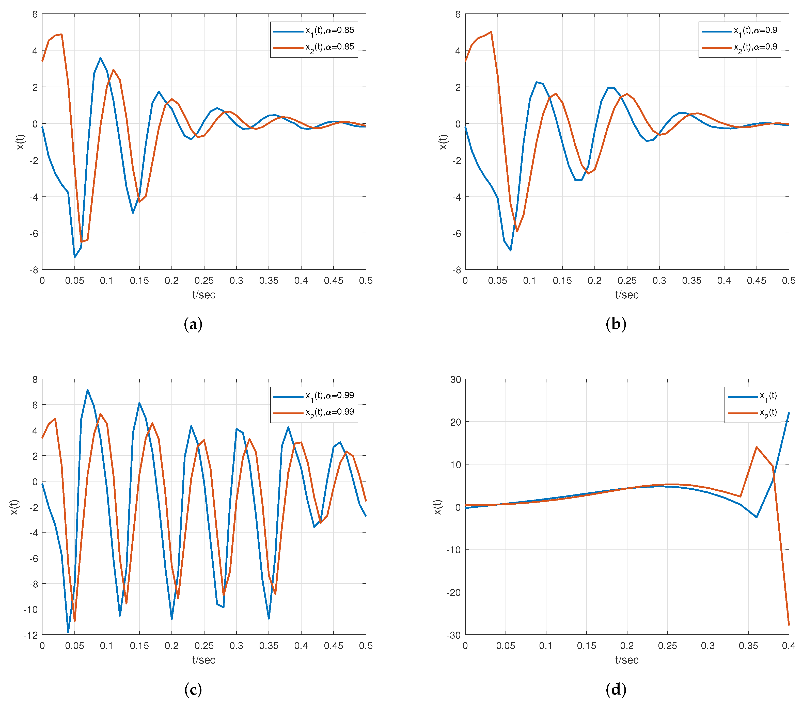
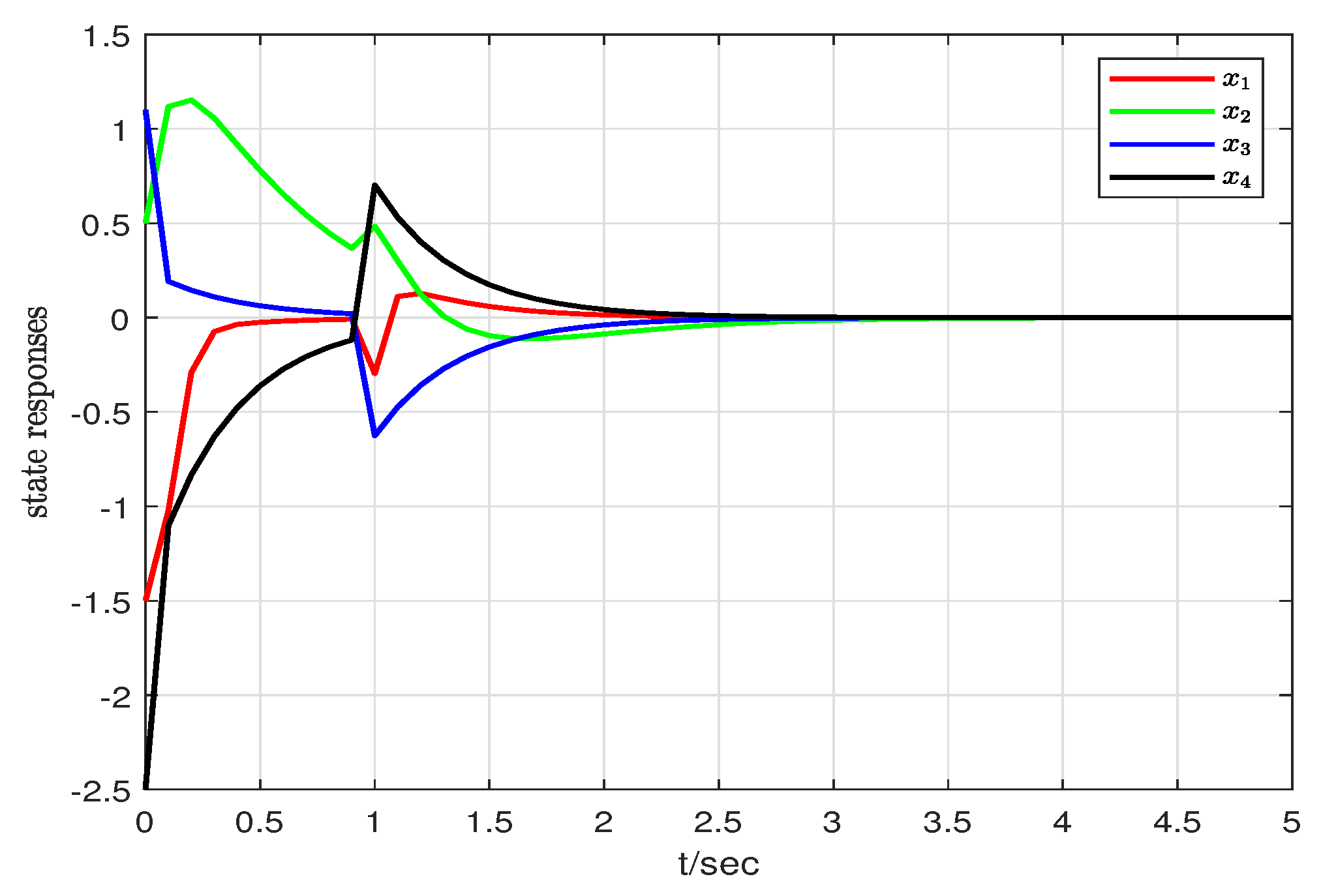
5. Simulation Results

In this part, numerical examples of FFONCS will be supplied for validation.
Example 1.
Let us consider the following dynamical delayed FFONCS:
C D α x ( t ) = i = 1 r h i θ ( t ) j = 1 r h j θ ( t k ) { A i ( t ) x ( t ) + A d i ( t ) x ( t τ ( t ) ) + B i ( t ) K j x ( t h ( t ) ) + w ( t ) } ,
where
A 1 = 5 0.2 0 4 , A 2 = 4 0.1 0 3 , A d 1 = 1 0.4 0.3 0.1 , A d 2 = 1 0.1 0.1 0.2 , B 1 = 0.5 0.7 0.7 0.4 , B 2 = 0.3 0.2 0.1 0.6 , Y 1 = Y 2 = 0.5 0 0 0.5 , ξ 11 = ξ 21 = ξ 31 = d i a g { 0.1 , 0.1 } , ξ 12 = ξ 22 = ξ 32 = d i a g { 0.2 , 0.2 } .
and the fuzzy membership functions are h 1 = 1 1 + e 2 x 1 ( t ) , h 2 = 1 h 1 . Suppose that τ ( t ) = 1 + 0.2 s i n t and the related time-delays are chosen as τ = 1.2 , μ = 0.2 , h ^ 1 = 0.1 , h ^ 2 = 0.2 , μ 1 = 0.1 , and the external disturbance w ( t ) is chosen as 0.5 e t . Using these values and solving the LMIs in Theorem 3 by standard software (MATLAB LMI toolbox), succeeding sections of the extended dissipative conditions for the FFONCS (35) are established. Furthermore, the extended dissipative condition includes L 2 L execution, passivity, H execution, mixed passivity and H execution and ( Q S R ) -dissipativity as unique instance. The weighting matrices χ 1 , χ 2 , χ 3 , and χ 4 are used in the extended dissipative study of system (35).
L 2 L performance: χ 1 = 0 , χ 2 = 0 , χ 3 = γ ˜ 2 I , χ 4 = I , and δ = 0 . Using the aforementioned parameters, we can get the subsequent gain by solving Theorem 3 and utilizing the standard software.
K 1 = 0.2630 0.0072 0.0103 0.0422 , K 2 = 0.2475 0.0241 0.0145 0.3014 .
Employing the effect of control gains and state variable responses of the system (35) under the randomized initial conditions which are depicted in Figure 2. It is easy to see that the states of the system are capable of keeping stable, behave L 2 L performance in accordance with the above-indicated parameter values, as shown in Figure 2a–c. Furthermore, the uncontrolled system state response curves are depicted in Figure 2d, indicating the performance of the proposed controller. We can notice that the numerical simulation results deliver better stability performance.
H execution: χ 1 = I , χ 2 = 0 , χ 3 = γ ˜ 2 I , χ 4 = 0 , and δ = 0 , it is simple to estimate the LMIs in Theorem 3, and the following gains are
K 1 = 0.3487 0.0032 0.0142 0.0533 , K 2 = 0.5421 0.0714 0.0514 0.1632 .
Simultaneously, the numerical simulation results are sketched in Figure 3a–c, which analyzes the following history of the state variable curves concerning the obtained gain matrices. The instability of the open-loop system (35) is depicted in Figure 3d. As a result, the system under examination operates admirably.
Passivity performance: χ 1 = 0 , χ 2 = I , χ 3 = γ ˜ I , χ 4 = 0 , and δ = 0 . The coordinated system analysis now shifts to passivity performance. To test the feasibility in Theorem 3, we generate the subsequent gain using the MATLAB LMI toolkit.
K 1 = 0.4511 0.0143 0.0326 0.0431 , K 2 = 0.6541 0.0245 0.1224 0.1121 .
Numerical simulation is given in Figure 4a–d. The resultant state response curves under random initial conditions with different fractional order conditions 0.85, 0.9, 0.99, and distraction w ( t ) that converge to zero coupled with the passivity performance and the consistency of available parameters has been shown in the Figure 4a–d. Figure 4d demonstrates the performance of the open-loop system (i.e., without control inputs). Which verifies the validation of the control strategy.
Mixed H and Passivity behavior: χ 1 = γ ˜ 1 α ˜ I , χ 2 = ( 1 α ˜ ) I , χ 3 = γ ˜ I , χ 4 = 0 with α ˜ = 0.5 . The prolonged dissipativity behavior is reduced to a combination of H and passivity behavior at this stage. By adopting the known parameter values and generating the gain value with Theorem 3 LMIs is
K 1 = 0.0854 0.1123 0.1431 0.3267 , K 2 = 0.1254 0.5541 0.6255 0.8741 .
The behavioral reactions of the system’s state response curves (35) with the control gain matrices given above are pictured in Figure 5a–c with the randomized initial conditions and therefore exhibit mixed H and passive behavior fulfilling the aforementioned mentioned requirements. It is discovered that controllers have a major impact on the unstable system nature.
( Q S R ) Dissipativity: χ 1 = Q , χ 2 = S , χ 3 = R γ ˜ I , and χ 4 = 0 with
Q = 1 0 0 1 , S = 0.3 0 0.4 0.25 , R = 0.3 0 0 0.3 .
Similarly, solving the Theorem 3 inequalities and applying the aforesaid parameters, the resultant gain matrices are as follows:
K 1 = 0.6069 0.0237 0.0414 1.1034 , K 2 = 0.7071 0.8274 1.0323 2.0124 ,
and the performance of the dissipativity parameter is α ˜ = 0.0072 . Meanwhile, the equivalent numerical simulation curves are presented in Figure 6a–d. Figure 6a–c represents the corresponding state response curves with the impact of u ( t ) under the randomised initial condition. Moreover, the Figure 6a–c are simulated with different α values 0.85 , 0.9 , 0.99 . From Figure 6d, we can see that the unforced system and it is not stable. In the numerical simulation behavior, it is pointed out that the considered unforced system is unstable but the forced system is stable through the designed control law. Thus, the results show that the designed feedback controller is suitable for stabilizing the system (35). As a result, the ( Q S R ) dissipativity performance demand is fulfilled. Moreover, Figure 6a–d reveals that our stabilization conditions.
Example 2.
Consider the single-link robot arm (SLRA) model and it can be described as follows:
φ ¨ ( t ) = M G L J s i n ( φ ( t ) ) D J φ ˙ ( t ) + 1 J u ( t ) + 1 J w ( t ) ,
where φ ( t ) is the arm angle position, u ( t ) is the system’ s input, and disturbance noted as w ( t ) . Mass of the payload is defined as M , a moment of inertia says as J , acceleration of gravity, length of the arm, and coefficient of viscous friction can be denoted as G , L , D respectively. We choose α = 0.5 , and create state variables as
x ( t ) = [ x 1 ( t ) x 2 ( t ) x 3 ( t ) x 4 ( t ) ] T , = [ θ ( t ) C D α x ( t ) θ ˙ ( t ) C D α x ( t ) ] T .
The nonlinear function s i n ( x 1 ( t ) ) may be represented using the same way as in [4] as
s i n ( x 1 ( t ) ) = h 1 ( x 1 ( t ) ) x 1 ( t ) + ν h 2 ( x 1 ( t ) ) x 1 ( t ) ,
the membership function h 1 ( x 1 ( t ) ) and h 2 ( x 1 ( t ) ) are obtained by
h 1 ( x 1 ( t ) ) = s i n ( x 1 ( t ) ) ν x 1 ( t ) x 1 ( t ) ( 1 ν ) , x 1 ( t ) 0 , 1 , x 1 ( t ) = 0 , h 2 ( x 1 ( t ) ) = x 1 ( t ) s i n ( x 1 ( t ) ) x 1 ( t ) ( 1 ν ) , x 1 ( t ) 0 , 1 , x 1 ( t ) = 0 ,
with the impact of time delay, we may describe the model (41) through the fuzzy approach.
Plant Rule 1:IF x 1 ( t ) is about 0 rad,THEN
C D α x ( t ) = ( A 1 ( t ) x ( t ) + A d 1 ( t ) x ( t τ ( t ) ) + B 1 K j x ( t h ( t ) ) + w ( t ) ) ,
Plant Rule 2:IF x 1 ( t ) is about π or π rad,THEN
C D α x ( t ) = ( A 2 ( t ) x ( t ) + A d 2 ( t ) x ( t τ ( t ) ) + B 2 K j x ( t h ( t ) ) + w ( t ) ) ,
where
A 1 = 0 1 0 0 0 0 1 0 0 0 0 1 G L 0 D 1 , A 2 = 0 1 0 0 0 0 1 0 0 0 0 1 ν G L 0 D 1 , A d 1 = 0.001 1 0 0 0 0.001 0.1 0 0 0 0.01 1 0 0 0 0.1 , B 1 = B 2 = 0 0 0 1 , A d 2 = 0.001 1 0 0 0 0.001 0.1 0 0 0 0.01 0.1 0 0 0 0.1 , Δ A i = Y i F i ( t ) ξ 1 i , Δ A d i = Y i F i ( t ) ξ 2 i , F 1 ( t ) = F 2 ( t ) = c o s t , Y 1 = [ 0.5 0 1 0 ] T , Y 2 = [ 1 0.5 0 0 ] T , ξ 11 = ξ 12 = [ 0.1 0.1 0.1 0.15 ] , ξ 21 = ξ 22 = [ 0.2 0.1 0.2 0.1 ] .
We choose the parameters as G = 9.8 , M = 1 , J = 1 , ν = 1 / 100 π , L = 0.5 , D = 0.2 , and time-varying delay τ ( t ) = 0.2 s i n t + 0.1 , h ^ 1 = 0.1 , h ^ 1 = 0.2 , μ 1 = 0.1 , and the external disturbance w ( t ) is chosen as 0.1 s i n t . In light of the conditions in Theorem 3, ensures the subsequent fuzzy control gains:
K 1 = [ 1.3842 12.6732 3.7503 1.8672 ] , K 2 = [ 4.8131 10.7312 1.3712 0.9732 ] .
The following simulation results are shown through the assumed initial conditions x ( 0 ) = [ 1.5 0.5 1.1 2.5 ] T . The state response curve of the closed-loop system in Example 2 by the controller designed in this study is shown in Figure 7. It becomes apparent that the developed fuzzy control stabilizes the system (36).

6. Conclusions

This research investigates the extended dissipativity analysis of a robust fuzzy delayed fractional-order network control system. The results have been developed to verify the quadratic stability and extended dissipativity of the investigated system by creating a suitable Lyapunov-Krasovskii functional and applying various inequality approaches. By giving appropriate simulation data, the usefulness of the controller design process has been established. Moreover, the results can be extended to the dynamic execution of FO discrete-time neural networks with event-triggered sampled data control [26,39,40,41] with imperfect communication, such as packet dropouts and quantization is worth further investigation in the future.

Author Contributions

Conceptualization, R.V. and P.H.; methodology and validation, N.G., R.V. and P.H.; investigation and formal analysis, K.C. and S.V.; software, S.V.; supervision, R.V. and K.C.; writing—original draft preparation, R.V.; writing—review and editing, N.G. and R.V. All authors have read and agreed to the published version of the manuscript.

Funding

This research received no external funding.

Data Availability Statement

Data sharing is not applicable to this article as no datasets were generated or analyzed during the current study.

Acknowledgments

We thank referees and editors for their valuable comments.

Conflicts of Interest

The author declares that there is no conflict of interest regarding the publication of this paper.

References

  1. Shen, J.; Lam, J. Stability and performance analysis for positive fractional-order systems with time-varying delays. IEEE Trans. Autom. Control 2015, 61, 2676–2681. [Google Scholar] [CrossRef]
  2. Manigandan, M.; Muthaiah, S.; Nandhagopal, T.; Vadivel, R.; Unyong, B.; Gunasekaran, N. Existence results for coupled system of nonlinear differential equations and inclusions involving sequential derivatives of fractional order. AIMS Math. 2022, 7, 723–755. [Google Scholar] [CrossRef]
  3. Phat, V.; Niamsup, P.; Thuan, M.V. A new design method for observer-based control of nonlinear fractional-order systems with time-variable delay. Eur. J. Control 2020, 56, 124–131. [Google Scholar] [CrossRef]
  4. Mohammadzadeh, A.; Ghaemi, S. Robust synchronization of uncertain fractional-order chaotic systems with time-varying delay. Nonlinear Dyn. 2018, 93, 1809–1821. [Google Scholar] [CrossRef]
  5. Thanh, N.T.; Phat, V.N. Improved approach for finite-time stability of nonlinear fractional-order systems with interval time-varying delay. IEEE Trans. Circuits Syst. II Express Briefs 2018, 66, 1356–1360. [Google Scholar] [CrossRef]
  6. Zhang, H.; Ye, M.; Cao, J.; Alsaedi, A. Synchronization control of Riemann-Liouville fractional competitive network systems with time-varying delay and different time scales. Int. J. Control Autom. Syst. 2018, 16, 1404–1414. [Google Scholar] [CrossRef]
  7. Liu, C.; Gong, Z.; Teo, K.L.; Wang, S. Optimal control of nonlinear fractional-order systems with multiple time-varying delays. J. Optim. Theory Appl. 2022, 193, 856–876. [Google Scholar] [CrossRef]
  8. Aghayan, Z.S.; Alfi, A.; Tenreiro Machado, J. Stability analysis of fractional order neutral-type systems considering time varying delays, nonlinear perturbations, and input saturation. Math. Methods Appl. Sci. 2020, 43, 10332–10345. [Google Scholar] [CrossRef]
  9. Zhou, Y.; Liu, H.; Cao, J.; Li, S. Composite learning fuzzy synchronization for incommensurate fractional-order chaotic systems with time-varying delays. Int. J. Adapt. Control Signal Process. 2019, 33, 1739–1758. [Google Scholar] [CrossRef]
  10. Mahmoudabadi, P.; Tavakoli-Kakhki, M. Improved stability criteria for nonlinear fractional order fuzzy systems with time-varying delay. Soft Comput. 2022, 26, 4215–4226. [Google Scholar] [CrossRef]
  11. Song, S.; Park, J.H.; Zhang, B.; Song, X. Observer-based adaptive hybrid fuzzy resilient control for fractional-order nonlinear systems with time-varying delays and actuator failures. IEEE Trans. Fuzzy Syst. 2019, 29, 471–485. [Google Scholar] [CrossRef]
  12. Karthick, S.; Sakthivel, R.; Ma, Y.K.; Mohanapriya, S.; Leelamani, A. Disturbance rejection of fractional-order TS fuzzy neural networks based on quantized dynamic output feedback controller. Appl. Math. Comput. 2019, 361, 846–857. [Google Scholar]
  13. Du, F.; Lu, J.G. Finite-time stability of fractional-order fuzzy cellular neural networks with time delays. Fuzzy Sets Syst. 2022, 438, 107–120. [Google Scholar] [CrossRef]
  14. Zhang, B.; Zhuang, J.; Liu, H.; Cao, J.; Xia, Y. Master–slave synchronization of a class of fractional-order Takagi–Sugeno fuzzy neural networks. Adv. Differ. Equ. 2018, 2018, 473. [Google Scholar] [CrossRef] [Green Version]
  15. Hao, Y.; Zhang, X. TS Fuzzy Control of Uncertain Fractional-Order Systems with Time Delay. J. Math. 2021, 2021, 6636882. [Google Scholar] [CrossRef]
  16. Sweetha, S.; Sakthivel, R.; Almakhles, D.; Priyanka, S. Non-Fragile Fault-Tolerant Control Design for Fractional-Order Nonlinear Systems with Distributed Delays and Fractional Parametric Uncertainties. IEEE Access 2022, 10, 19997–20007. [Google Scholar] [CrossRef]
  17. Hua, C.; Zhang, T.; Li, Y.; Guan, X. Robust output feedback control for fractional order nonlinear systems with time-varying delays. IEEE/CAA J. Autom. Sin. 2016, 3, 477–482. [Google Scholar]
  18. Liu, H.; Xie, G.; Gao, Y. Containment control of fractional-order multi-agent systems with time-varying delays. J. Frankl. Inst. 2019, 356, 9992–10014. [Google Scholar] [CrossRef]
  19. Chen, L.; Wu, R.; Yuan, L.; Yin, L.; Chen, Y.; Xu, S. Guaranteed cost control of fractional-order linear uncertain systems with time-varying delay. Optim. Control Appl. Methods 2021, 42, 1102–1118. [Google Scholar] [CrossRef]
  20. Hespanha, J.P.; Naghshtabrizi, P.; Xu, Y. A survey of recent results in networked control systems. Proc. IEEE 2007, 95, 138–162. [Google Scholar] [CrossRef] [Green Version]
  21. Zhang, W.A.; Yu, L. A robust control approach to stabilization of networked control systems with time-varying delays. Automatica 2009, 45, 2440–2445. [Google Scholar] [CrossRef]
  22. Peng, C.; Tian, Y.C.; Tade, M.O. State feedback controller design of networked control systems with interval time-varying delay and nonlinearity. Int. J. Robust Nonlinear Control IFAC-Affil. J. 2008, 18, 1285–1301. [Google Scholar] [CrossRef]
  23. Song, X.; Tejado, I.; Chen, Y. Stabilization for fractional-order networked control systems with input time-varying delays. In Proceedings of the 2011 International Conference on Advanced Mechatronic Systems, Zhengzhou, China, 11–13 August 2011; pp. 39–42. [Google Scholar]
  24. Zhang, B.; Zheng, W.X.; Xu, S. Filtering of Markovian jump delay systems based on a new performance index. IEEE Trans. Circuits Syst. I Regul. Pap. 2013, 60, 1250–1263. [Google Scholar] [CrossRef]
  25. Ali, M.S.; Vadivel, R.; Alsaedi, A.; Ahmad, B. Extended dissipativity and event-triggered synchronization for T–S fuzzy Markovian jumping delayed stochastic neural networks with leakage delays via fault-tolerant control. Soft Comput. 2020, 24, 3675–3694. [Google Scholar] [CrossRef]
  26. Vadivel, R.; Hammachukiattikul, P.; Gunasekaran, N.; Saravanakumar, R.; Dutta, H. Strict dissipativity synchronization for delayed static neural networks: An event-triggered scheme. Chaos Solitons Fractals 2021, 150, 111212. [Google Scholar] [CrossRef]
  27. Anbuvithya, R.; Sri, S.D.; Vadivel, R.; Gunasekaran, N.; Hammachukiattikul, P. Extended dissipativity and non-fragile synchronization for recurrent neural networks with multiple time-varying delays via sampled-data control. IEEE Access 2021, 9, 31454–31466. [Google Scholar] [CrossRef]
  28. Podlubny, I. Fractional Differential Equations: An Introduction to Fractional Derivatives, Fractional Differential Equations, to Methods of Their Solution and Some of Their Applications; Elsevier: Amsterdam, The Netherlands, 1998. [Google Scholar]
  29. Wang, L.; Lam, H.K. A new approach to stability and stabilization analysis for continuous-time Takagi–Sugeno fuzzy systems with time delay. IEEE Trans. Fuzzy Syst. 2017, 26, 2460–2465. [Google Scholar] [CrossRef] [Green Version]
  30. Gu, K.; Chen, J.; Kharitonov, V.L. Stability of Time-Delay Systems; Springer Science & Business Media: Berlin/Heidelberg, Germany, 2003. [Google Scholar]
  31. Aguila-Camacho, N.; Duarte-Mermoud, M.A.; Gallegos, J.A. Lyapunov functions for fractional order systems. Commun. Nonlinear Sci. Numer. Simul. 2014, 19, 2951–2957. [Google Scholar] [CrossRef]
  32. Ali, M.S.; Narayanan, G.; Nahavandi, S.; Wang, J.L.; Cao, J. Global dissipativity analysis and stability analysis for fractional-order quaternion-valued neural networks with time delays. IEEE Trans. Syst. Man Cybern. Syst. 2021, 52, 4046–4056. [Google Scholar] [CrossRef]
  33. Shafiya, M.; Nagamani, G. Extended dissipativity criterion for fractional-order neural networks with time-varying parameter and interval uncertainties. Comput. Appl. Math. 2022, 41, 95. [Google Scholar] [CrossRef]
  34. Thi Hong, D.; Huu Sau, N.; Viet Thuan, M. Output feedback finite-time dissipative control for uncertain nonlinear fractional-order systems. Asian J. Control 2021, 24, 2284–2293. [Google Scholar] [CrossRef]
  35. Ji, Y.; Su, L.; Qiu, J. Design of fuzzy output feedback stabilization for uncertain fractional-order systems. Neurocomputing 2016, 173, 1683–1693. [Google Scholar] [CrossRef]
  36. Lin, C.; Chen, B.; Wang, Q.G. Static output feedback stabilization for fractional-order systems in T-S fuzzy models. Neurocomputing 2016, 218, 354–358. [Google Scholar] [CrossRef]
  37. Zhang, X.; Wang, Z. Stabilisation of Takagi–Sugeno fuzzy singular fractional-order systems subject to actuator saturation. Int. J. Syst. Sci. 2020, 51, 3225–3236. [Google Scholar] [CrossRef]
  38. Liu, H.; Pan, Y.; Cao, J.; Zhou, Y.; Wang, H. Positivity and stability analysis for fractional-order delayed systems: A T-S fuzzy model approach. IEEE Trans. Fuzzy Syst. 2020, 29, 927–939. [Google Scholar] [CrossRef]
  39. Senan, S.; Ali, M.S.; Vadivel, R.; Arik, S. Decentralized event-triggered synchronization of uncertain Markovian jumping neutral-type neural networks with mixed delays. Neural Netw. 2017, 86, 32–41. [Google Scholar] [CrossRef]
  40. Vadivel, R.; Srinivasan, S.; Wu, Y.; Gunasekaran, N. Study on bifurcation analysis and Takagi–Sugeno fuzzy sampled-data stabilization of permanent magnet synchronous motor systems. Math. Methods Appl. Sci. 2021. [Google Scholar] [CrossRef]
  41. Vadivel, R.; Suresh, R.; Hammachukiattikul, P.; Unyong, B.; Gunasekaran, N. Event-Triggered Filtering for Network-Based Neutral Systems With Time-Varying Delays via TS Fuzzy Approach. IEEE Access 2021, 9, 145133–145147. [Google Scholar] [CrossRef]
Figure 1. Schematic diagram for fractional order networked control system.
Fractalfract 06 00591 g001
Figure 2. The panels (ac) contain the trajectories of the state variable x 1 ( t ) and x 2 ( t ) for L 2 L performance with distinct FO circumstances α = 0.85 , 0.9 , 0.99 . Moreover, panel (d) is the trajectories of the open loop system in Example 1.
Fractalfract 06 00591 g002
Figure 3. The panels (ac) contain the curves of the state variable x 1 ( t ) and x 2 ( t ) for H performance with distinct FO circumstances α = 0.85 , 0.9 , 0.99 . Moreover, the panel (d) is the trajectories of the open loop system in Example 1.
Fractalfract 06 00591 g003aFractalfract 06 00591 g003b
Figure 4. The panels (ac) contain the curves of state variable x 1 ( t ) and x 2 ( t ) for passivity execution with distinct FO circumstances α = 0.85 , 0.9 , 0.99 . Moreover, panel (d) is the trajectories of the open loop system in Example 1.
Fractalfract 06 00591 g004aFractalfract 06 00591 g004b
Figure 5. The panels (ac) contain the curves of state variable x 1 ( t ) and x 2 ( t ) for mixed H and Passivity performance with distinct FO circumstances α = 0.85 , 0.9 , 0.99 . Moreover, panel (d) is the trajectories of the open loop system in Example 1.
Fractalfract 06 00591 g005
Figure 6. The panels (ac) contain the curves of state variable x 1 ( t ) and x 2 ( t ) for ( Q S R ) dissipativity efficacy with distinct FO circumstances α = 0.85 , 0.9 , 0.99 . Moreover, panel (d) is the trajectories of the open loop system in Example 1.
Fractalfract 06 00591 g006
Figure 7. Stability behavior for FO condition α = 0.85 in Example 2.
Fractalfract 06 00591 g007
Publisher’s Note: MDPI stays neutral with regard to jurisdictional claims in published maps and institutional affiliations.

