Article

Analysis of Lie Symmetries with Conservation Laws and Solutions of Generalized (4 + 1)-Dimensional Time-Fractional Fokas Equation

1
College of Mathematics and Systems Science, Shandong University of Science and Technology, Qingdao 266590, China
2
Division of Mathematics and Artificial Intelligence, Qilu University of Technology (Shandong Academy of Sciences), Jinan 250353, China
*
Author to whom correspondence should be addressed.
Fractal Fract. 2022, 6(2), 108; https://doi.org/10.3390/fractalfract6020108
Submission received: 11 January 2022 / Revised: 7 February 2022 / Accepted: 10 February 2022 / Published: 13 February 2022
(This article belongs to the Special Issue Recent Advances in Computational Physics with Fractional Application)

Abstract

:
High-dimensional fractional equations research is a cutting-edge field with significant practical and theoretical implications in mathematics, physics, biological fluid mechanics, and other fields. Firstly, in this paper, the (4 + 1)-dimensional time-fractional Fokas equation in a higher-dimensional integrable system is studied by using semi-inverse and fractional variational theory. Then, the Lie symmetry analysis and conservation law analysis are carried out for the higher dimensional fractional order model with the symmetry of fractional order. Finally, the fractional-order equation is solved using the bilinear approach to produce the rogue wave and multi-soliton solutions, and the fractional equation is numerically solved using the Radial Basis Functions (RBFs) method.

1. Introduction

Fractional calculus [1,2] is a new research field in science and engineering, and it is widely used in physical mathematics, medicine, signal processing, liquid and gas fluctuation, and other fields. The concept of fractional order calculus [3,4] dates back to 1695, and the half-derivative was first mentioned in Leibniz’s letter to L’Hospital. Then, in 1730, Euler suggested that the non-integer p-order derivative d ρ x σ d x ρ of x σ was meaningful. In 1822, Fourier proposed the following formula:
d ρ x σ d x ρ = 1 2 π λ ρ d λ f ( t ) cos λ x t λ + ρ π 2 d t .
Compared with integer calculus, fractional calculus are non-local, and compared with classical calculus, fractional calculus has the properties of memory, long-distance interaction and inheritance, which are the main advantages of fractional calculus. The conceptual theory of fractional derivatives [5] is more suitable for modeling, which has allowed fractional differential equations to be gradually applied to all fields of research, and its practicability and accuracy are becoming stronger and stronger. In this paper, the high-dimensional Fokas equation is transformed into the high-dimensional time-fractional Fokas equation.
The creation of accurate solutions to high-dimensional nonlinear PDE equations [6,7,8] is crucial for comprehending some things that cannot be noted firsthand. However, it is generally difficult to gain control over high-dimensional nonlinear dynamical systems. In this paper, we will research the high-dimensional Fokas equation. Fokas [9] extended the integrable Kadomtsev–Petviashvili (KP) and Davey–Stewartson (DS) equations to present a new (4 + 1)-dimensional non-linear wave equation which is presented as
u x t 1 4 u x x x y + 1 4 u x y y y + 3 2 u 2 x y 3 2 u z w = 0 .
It is a generalization of DS equation [10,11], (2 + 1)-dimensional KdV equation and KP equation [12], and it contains 4-dimensional space scale and 1-dimensional time scale. DS equation and KP equation have been widely used in mathematical physics, so the (4 + 1)-dimensional Fokas equation can be used to describe wave problems [13,14] in physics, such as surface waves and internal waves [15,16].
In recent years, many methods have been used to construct exact solutions of nonlinear problems, such as homotopy perturbation method [17], Exp-function method [18], hyperbolic tangent method, variational iterative method [19], and so on. Some scholars have studied the exact solution of the (4 + 1)-dimensional Fokas equation. Demiray et al. [20] obtained the hyperbolic function solution and dark soliton solution of the (4 + 1)-dimensional Fokas equation by using the improved exp ( Ω ( ξ ) ) -expansion function method. Using the extended f expansion method and its deformation, He [21] obtained some new exact solutions of the (4 + 1)-dimensional Fokas equation expressed by Jacobi elliptic function, weerstrass elliptic function, hyperbolic function and trigonometric function. Lee et al. [22] obtained the exact traveling wave solution by symbolic calculation, and obtained the doubly periodic wave solution by using the generalized Jacobi elliptic function method. It is also worth paying attention to Wazwaz [23] who used Hirota bilinear method to solve the multi-soliton solution of KP equation; Tian et al. [24] used the Hirota bilinear method to solve the lump-type solution, interaction solution and periodic wave solution of KdV equation, Tajiri [25] discusses the stability of solitons of the DS equation by Hirota method. In this paper, we extend the bilinear method [26,27] to the (4 + 1)-dimensional time-fractional Fokas equation, and obtain the rogue wave solutions and n-soliton solutions [28,29].
Rogue waves [30,31] have a large amplitude, sharp waveform and short duration. Rogue waves show a local structure in time and space, which can gather huge energy in a short time, which gives them strong destructive power. At present, there is no unified definition of rogue waves. Most scholars believe that rogue wave refers to a wave whose peak is at least twice as high as a plane wave, appears for a very short time and has strong destructive power. As rogue waves have these characteristics different from other nonlinear waves, rogue waves have become a research hotspot in the fields of ocean atmosphere, plasma and Bose–Einstein condensation in recent years. The research results obtained in this paper hope to enrich the dynamic behavior of high-dimensional nonlinear evolution equations [32], such as the (4 + 1)-dimensional nonlinear wave field.
In addition, we not only obtain the exact solution of the equation, but also study its numerical solution. By reviewing the literature, we found that the finite difference method of finite element method and grid method can be used to solve partial differential equations. However, in practical application, we find that the accuracy of the solution obtained by this method is low. Therefore, we need to use meshless technology [33] to obtain higher precision solutions. The numerical solution of the time-fractional Fokas equation is obtained using the Radial Basis Function (RBF) method [34] in this work.
For differential equation modeling, symmetry and conservation rules [35] are extremely important. Lie symmetry [36,37,38] is a systematic and effective method to study partial differential equations. It was first proposed by the Norwegian mathematician Lie [39] at the end of the 19th century. Lie symmetry analysis provides an effective and powerful tool for determining boundary value problems, initial value problems and conservation laws of differential equations [40]. At the beginning of the 21st century, Gazizov et al. studied the symmetry of time-fractional ordinary differential equations and the symmetry of time-fractional ordinary differential equations [41]. In recent years, many scholars have studied time-fractional partial differential equations by lie symmetry, but there are few studies in high-dimensional high-order partial differential systems. In this paper, Lie symmetry analysis is conducted for the high-dimensional and high-order time-fractional order Fokas equation. Conservation laws are of great significance for analyzing the integrability and internal properties of differential equations and proving the existence and uniqueness of solutions. The symmetry and conservation laws of differential equations are connected by Noether’s theorem, and the relationship between them leads to the further development of conservation laws.
The structure of this paper is designed as follows. In Section 2, by using the semi-inverse method and the fractional variational principle [42,43], we derive the (4 + 1)-dimensional time-fractional Fokas equation. Using the Lie symmetry analysis method, we discuss the conservation laws of the time-fractional Fokas equation in Section 3. In Section 4, we use the simplified bilinear method to obtain the rogue wave solution and soliton solution of (4 + 1)-dimensional time-fractional order Fokas. Finally, in Section 5, the numerical solution of the (4 + 1)-dimensional time-fractional Fokas equation is obtained by using the RBF method, and an examination of absolute inaccuracy under various scenarios is provided.

2. Derivation of (4 + 1)-Dimensional Time Fraction Fokas Equation

The integer order equation is extended to the fractional order form using the semi-inverse method and the fractional variational principle based on the definition of Riemann–Liouville fractional derivative, and the (4 + 1)-dimension time-fractional order Fokas equation is obtained.
The (4 + 1)-dimensional Fokas equation is written as follows:
4 u t x u x x x y + u x y y y + 12 u x u y + 12 u u x y 6 u z w = 0 .
Definition 1.
The ω Riemann–Liouville fractional derivative of the function u t is defined as follows [44,45]:
D t ω = n u t n , ω = n , n N , 1 Γ ( n ω ) n T n 0 t f ( t τ ) n ω 1 u ( x , τ ) d τ , n 1 < ω < n .
Definition 2.
Fractional integration by parts is defined as
c d ( d τ ) γ f ( t ) D t γ g ( t ) = Γ ( 1 + γ ) g ( t ) f ( t ) c d c d ( d t ) γ g ( t ) D t γ f ( t ) ,
where c t ( d τ ) γ f ( τ ) = γ c t d τ ( t τ ) r , f ( t ) , g ( t ) [ c , d ] .
Assuming that u ( x , y , z , w , t ) = v x ( x , y , z , w , t ) , v x ( x , y , z , w , t ) is the potential function, then the potential equation of the (4 + 1)-dimensional time-fractional Fokas equation is
4 v x x t v x x x x y + v x x y y y + 12 ( v x v x y ) x 6 v x z w = 0 .
Next, the semi-inverse method is used to derive the Lagrange form of Equation (1). The functional form of Equation (1) can be expressed as
J ( v ) = R d x Y d y Z d z T d t W d w v 4 c 1 v x x t c 2 v x x x x y + c 3 v x x y y y + 6 c 4 ( v x ) 2 x y 6 c 5 v x z w ,
where c i ( i = 1 , 2 , 3 , 4 , 5 , 6 ) are the Lagrange multiplier [46].
Using the integration by parts method, assuming v x | R = v y | Y = v z | Z = v w | W = v t | T = 0 , according to Equation (5), we obtain
J ( v ) = R d x Y d y Z d z T d t W d w [ 4 c 1 v x v x t + c 2 v x v x x x y c 3 v x v x y y y 12 c 4 ( v x ) 2 v x y + 6 c 5 v x v z w ] ,
In order to obtain the optimal result, the Lagrange multiplier c i ( i = 1 , 2 , 3 , 4 , 5 , 6 ) can be determined by the variation of Equation (6). We use the variational optimal conditions to integrate term by term, and achieve the following relationship.
F x , y , t , z , w , v x , v x t , v z w , v x y , v x x x y , v x y y y = F v x ( F v x ) 2 x y ( F v x y ) 2 x t ( F v x t ) 2 z w ( F v z w ) 4 x 3 y ( F v x x x y ) 4 x y 3 ( F v x y y y ) = 8 c 1 v x x t 2 c 2 v x x x x y + 2 c 3 v x x y y y + 24 c 4 ( v x 2 ) x y 12 c 5 v x z w = 0 .
Obviously, Equation (7) is equivalent to Equation (4). Therefore, the Lagrange multiplier is as follows:
c 1 = c 2 = c 3 = c 4 = c 5 = 1 2
We obtain the Lagrange form of the Fokas equation of integer order as follows:
L ( v , v x , v t , v y , v x x , v x y , v z w , v x x x y , v x y y y ) = 2 v t v x x + 1 2 v x v x x x y 1 2 v x v x y y y 6 v x 2 v x y + 3 v x v z w ,
Similarly, the Lagrange form of the fractional Fokas equation is as follows:
F ( v , v x , D t α v , v y , v x x , v x y , v z w , v x x x y , v x y y y ) = 2 D t α v v x x + 1 2 v x v x x x y 1 2 v x v x y y y 6 v x 2 v x y + 3 v x v z w ,
The functional form of the (4 + 1)-dimensional time-fractional Fokas equation is:
J ( v ) = R d x Y d y Z d z W d w T ( d t ) α F ( v , v x , D t α v , v y , v x x , v x y , v z w , v x x x y , v x y y y ) ,
in which
a t ( d τ ) γ f ( τ ) = γ a t d τ ( t τ ) γ f ( τ ) .
According to Definition 2, the Euler–Lagrange equation of the time-fractional Fokas equation is as follows:
( F v ) v + ( F v x ) v x + ( F D t α v ) D t α v + ( F v y ) v y + ( F v x x ) v x x + ( F v x y ) v x y + ( F v z w ) v z w + ( F v x x x y ) v x x x y + ( F v x y y y ) v x y y y = 0 ,
Substituting Equation (9) into Equation (12), and according to the definition of fractional potential function, we use the formula D x β v ( x , y , z , w , t ) = u ( x , y , z , w , t ) , then we obtain:
4 D t α u x u x x x y + u x y y y + 12 u x u y + 12 u u x y 6 u z w = 0 .
Compared with the integer order model, the Equation (13) is more general and has potential value for the study of some properties in practical problems.

3. Conservation Laws and Lie Symmetry Analysis of (4 + 1)-Dimensional Time-Fractional Order Fokas Equations

3.1. Lie Symmetry Analysis

Definition 3.
The broad definition of Leibniz’s rule is as follows [47],
D t σ ( Ξ ( t ) σ ( t ) ) = n = 0 α n D t σ n Ξ ( t ) D t n σ ( t ) , σ > 0 .
where D t σ is the total fractional derivative operator, and
σ n = ( 1 ) n 1 σ Γ ( n σ ) Γ ( 1 σ ) Γ ( n + 1 )
Definition 4.
The generalized chain rule is defined as follows [48],
d m ( Ξ ( t ) ) d t m = k = 0 m r = 0 k k r 1 k ! [ y ( t ) ] r d m d t m ( y ( t ) ) k r d k ( y ) d y k .
The time-fractional Fokas equation here has five independent variables
F ( x , y , z , w , t , v , v x , t σ v x , v y , v x x , v x y , v z w , v x x x y , v x y y y ) = 0 , σ > 0 ,
where the subscript represents the partial derivative. The infinitesimal transformation is defined as
x * = x + ϵ ξ 1 ( x , y , z , w , t , u ) + o ( ϵ 2 ) , y * = y + ϵ ξ 2 ( x , y , z , w , t , u ) + o ( ϵ 2 ) , z * = z + ϵ ξ 3 ( x , y , z , w , t , u ) + o ( ϵ 2 ) , w * = w + ϵ ξ 4 ( x , y , z , w , t , u ) + o ( ϵ 2 ) , t * = t + ϵ τ ( x , y , z , w , t , u ) + o ( ϵ 2 ) , u * = u + ϵ η ( x , y , z , w , t , u ) + o ( ϵ 2 ) , u * x * = u x + ϵ η x ( x , y , z , w , t , u ) + o ( ϵ 2 ) , u * y * = u y + ϵ η y ( x , y , z , w , t , u ) + o ( ϵ 2 ) , 2 u * x * y * = 2 u x y + ϵ η x y ( x , y , z , w , t , u ) + o ( ϵ 2 ) , 2 u * z * w * = 2 u z w + ϵ η z w ( x , y , z , w , t , u ) + o ( ϵ 2 ) , 4 u * x * 3 y * = 4 u x 3 y + ϵ η x x x y ( x , y , z , w , t , u ) + o ( ϵ 2 ) , 4 u * x * y * 3 = 4 u x y 3 + ϵ η x y y y ( x , y , z , w , t , u ) + o ( ϵ 2 ) , σ u x * t * σ = σ u x t σ + ϵ η σ t ( x , y , z , w , t , u ) + o ( ϵ 2 ) ,
where ϵ 1 is the parameter, ξ 1 , ξ 2 , ξ 3 , ξ 4 , τ , η are the subfunction, and η x , η y , η x y , η z w , η x x x y , η x y y y , η σ , t . Furthermore, the extended infinitesimal η x , η y , η x y , η z w , η x x x y , η x y y y , η σ , t have the forms:
η x = D x ( η ) u x D x ξ 1 u y D x ξ 2 u t D x ( τ ) u z D x ξ 3 u w D x ξ 4 , η y = D x ( η ) u y D y ξ 2 u x D y ξ 1 u t D y ( τ ) u z D y ξ 3 u w D y ξ 4 , η x y = D y η x u x x D y ξ 1 u x y D y ξ 2 u x t D y ( τ ) u x z D y ξ 3 u x w D y ξ 4 , η z w = D w η z u z x D w ξ 1 u z y D w ξ 2 u z t D w ( τ ) u z z D w ξ 3 u z w D w ξ 4 , η x x x y = D y η x x x u x x x x D y ξ 1 u x x x y D y ξ 2 u x x x t D y ( τ ) u x x x z D y ξ 3 u x x x w D y ξ 4 , η x y y y = D x η y y y u y y y x D x ξ 1 u y y y y D x ξ 2 u y y y t D x ( τ ) u y y y z D x ξ 3 u y y y w D x ξ 4 , η σ , t = D t σ η x + ξ 1 D t σ ξ 1 u x x D t σ ξ 1 u x x + ξ 2 D t σ u x y D t σ ξ 2 u x y + ξ 3 D t σ u x z D t σ ξ 3 u x z + ξ 4 D t σ u x w D t σ ξ 4 u x w + D t σ D t ( τ ) u x D t σ + 1 τ u x + τ D t σ + 1 u x ,
where D t σ is the total fractional derivative operator, and the total derivative D x , D y , D z , D t , D w are defined as
D t = t + u t u + u t t u t + u t x u x + u t y u y + , D x = x + u x u + u x x u x + u x t u t + u x y u y + , D y = y + u y u + u y y u y + u y x u x + u y t u t + , D z = z + u z u + u z z u z + u z x u x + u z t u t + , D w = w + u w u + u w w u w + u w x u x + u w t u t + .
With the generalized Leibnitz rule and the chain rule of composite functions, we can obtain:
η σ τ = σ η t σ + η u σ D t ξ 2 σ u t σ u σ η u t σ n = 1 σ n D t n ξ 1 D t σ n u x + n = 1 σ n α η u t α σ n + 1 D t n + 1 ξ 2 D t σ n ( u ) + R a ,
where
R a = n = 2 m = 2 n k = 2 m r = 0 k 1 σ n n m k r 1 k ! t n σ Γ ( n + 1 σ ) [ u ] r m t m u k r n m + k t n m u k .
With f ( t ) = 1 , we have
η x = η x + u x η u u x ξ 1 x u x 2 ξ 1 u u y ξ 2 x u y u x ξ 2 u u z ξ 3 x u z u x ξ 3 u u t τ x u t u x τ u u w ξ 4 x u w u x ξ 4 u , η y = η y + u y η u u y ξ 2 y u y 2 ξ 2 u u x ξ 1 y u x u y ξ 1 u u z ξ 3 y u z u y ξ 3 u u t τ y u t u y τ u u w ξ 4 y u w u y ξ 4 u , η z = η z + u z η u u z ξ 3 z u z 2 ξ 3 u u x ξ 1 z u x u z ξ 1 u u y ξ 2 z u y u z ξ 2 u u t τ z u t u z τ u u w ξ 4 z u w u z ξ 4 u , η x y = D y ( η x ) u x x D y ( ξ 1 ) u x y D y ( ξ 2 ) u x t D y ( τ ) u x z D y ( ξ 3 ) u x w D y ( ξ 4 ) = η x y + u y η x u + 2 u x y η u + u x η u y + u y u x η u u 2 u x y ξ 1 x u x ξ 1 x y u y u x ξ 1 x u 4 u x u x y ξ 1 u u x 2 ξ 1 u y u y u x 2 ξ 1 u u 2 u y y ξ 2 x u y ξ 2 x y u y 2 ξ 2 u x 2 u y y u x ξ 2 u 3 u y u x y ξ 2 u u y u x ξ 2 u y u y 2 u x ξ 2 u u 2 u z y ξ 3 x u z ξ 3 x y u y u z ξ 3 u x 2 u z y u x ξ 3 u 2 u z u x y ξ 3 u u z u x ξ 3 u y u z u x u y ξ 3 u u 2 u t y τ x u t τ x y u y u t τ u x 2 u t y u x τ u 2 u t u x y τ u u t u x τ u y u t u x u y τ u u 2 u w y ξ 4 x u w ξ 4 x y u y u w ξ 4 u x 2 u w y u x ξ 4 u 2 u w u x y ξ 4 u u w u x ξ 4 u y u w u x u y ξ 4 u u u x x ξ 1 y u x x u y ξ 1 u u x y ξ 2 y u x t τ y u x t u y τ u u x z ξ 3 y u x z u y ξ 3 u u x w ξ 4 y u x w u y ξ 4 u ,
η z w = D w ( η z ) u z x D w ( ξ 1 ) u z y D w ( ξ 2 ) u z t D w ( τ ) u z z D w ( ξ 3 ) u z w D w ( ξ 4 ) = η z w + u w η z u + 2 u z w η u + u z η u w + u w u z η u u 2 u z w ξ 3 z u z ξ 3 z w u w u z ξ 3 u z 4 u z u z w ξ 3 u u z 2 ξ 3 u w u y u z 2 ξ 3 u u 2 u x w ξ 1 z u x ξ 1 z w u x u w ξ 1 u z 2 u x w u z ξ 1 u u x u z w ξ 1 u u x u z ξ 1 u w u x u z u w ξ 1 u u 2 u y w ξ 2 z u y ξ 2 z w u y u w ξ 2 u z 2 u y w u z ξ 2 u 2 u y u z w ξ 2 u u y u z ξ 2 u w u y u z u w ξ 2 u u 2 u t w τ z u t τ z w u t u w τ u z 2 u t w u z τ u 2 u t u z w τ u u t u z τ u w u t u z u w τ u u 2 u w w ξ 4 z u w ξ 4 z w u w 2 ξ 4 u z 2 u w w u z ξ 4 u 2 u w u z w ξ 4 u u w u z ξ 4 u w 2 u w 2 u z ξ 4 u u u z x ξ 1 w u z x u w ξ 1 u u z y ξ 2 w u z y u w ξ 2 u u z t τ w u z t u w τ u u z z ξ 3 w u z z u w ξ 3 u u z w ξ 4 w u z w u w ξ 4 u ,
η x x x y = D x ( η x x y ) u x x x y D x ( ξ 1 ) u x x y y D x ( ξ 2 ) u x x y t D x ( τ ) u x x y z D x ( ξ 3 ) u x x y w D x ( ξ 4 ) = η x x x y + 3 u x η u x x y + 6 u x x η u x y + 3 u x 2 η u u x y + 12 u x x y η u x + 6 u x y η u x x + 12 u x u x y η u u x + u y η u x x x + 3 u x u y η u u x x + 4 u x x u y η u u x + 3 u x 2 u y η u u u x + 8 u x x x y η u + 12 u x u x x y η u u + 8 u x x u x y η u u + 6 u x 2 u x y η u u u + 4 u x x x η u y + 6 u x u x x η u u y + u x 3 η u u y + 4 u x y 2 η u u + 4 u y u x x y η u u + 2 u y u x y η u u x + 6 u x u y u x y η u u u + u y u x 3 η u u u u 11 u x x x y ξ 1 x 9 u x x y ξ 1 x x 30 u x u x x y ξ 1 u x 2 u x y ξ 1 x x x 12 u x u x y ξ 1 u x x 27 u x x u x y ξ 1 u x 18 u x 2 u x y ξ 1 u u x 8 u x x x ξ 1 x y 5 u x x ξ 1 x x y +
η x y y y = D y ( η x y y ) u x x y y D y ( ξ 1 ) u x y y y D y ( ξ 2 ) u x y y t D y ( τ ) u x y y z D y ( ξ 3 ) u x y y w D y ( ξ 4 ) , = η x y y y + 3 u y η u x y y + 6 u y y η u x y + 3 u y 2 η u u x y + 4 u y y y η u x + 6 u y u y y η u u x + u y 3 η u u u x + 8 u u y y y η u + 12 u x y y η u y + 12 u y u x y y η u u + 6 u x y η u y y + 12 u y u x y η u u y + 12 u y y u x y η u u + 6 u y 2 u x y η u u u + u x η u y y y + 3 u x u y η u u y y + 6 u x u y y η u u y + 3 u x u y 2 η u u u y + 4 u y y y u x η u u + 6 u x u y u y y η u u u + 3 u x u y 3 η u u u u 8 u x y y y ξ 1 x 12 u x y y ξ 1 x y 12 u y u x y y ξ 1 u x 6 u x y ξ 1 x y y 12 u y u x y ξ 1 u x y 12 u y y u x y ξ 1 u x 6 u y 2 u x y ξ 1 u u x u x ξ 1 x y y y 3 u x u y ξ 1 u x y y 6 u x u y y ξ 1 u x y + ,
η σ , t = t σ η x + η x u σ D t ( τ ) t σ u u t σ η x u + μ + n = 1 σ n t n η x u σ n + 1 D t n + 1 ( τ ) t σ n u n = 1 σ n D t n ξ 1 t σ n u x x n = 1 σ n D t n ξ 2 t σ n u x y n = 1 σ n D t n ξ 3 t σ n u x z n = 1 σ n D t n ξ 4 t σ n u x w .
The infinitesimal generator X is obtained by Lie symmetry theory:
X = ξ 1 ( x , y , z , w , t , u ) x + ξ 2 ( x , y , z , w , t , u ) y + ξ 3 ( x , y , z , w , t , u ) z + ξ 4 ( x , y , z , w , t , u ) z + τ ( x , y , z , w , t , u ) t + η ( x , y , z , w , t , u ) u
According to the infinitesimal invariance, Equation (14) is possible to write as
P r ( n ) X ( Δ ) Δ = 0 = 0 , n = 1 , 2 , 3 , , Δ = 4 D t σ u x u x x x y + u x y y y + 12 u x u y + 12 u u x y 6 u z w .
From Equations (16) and (19), we obtain the following operator
p r σ X = X + η x u x + η y u y + η x y u x y + η z w u z w + η x x x y u x x x y + η σ , t σ D t σ u x + ,
and from Equation (18), we can get
4 η σ , t + η ( 12 u x y ) + η x ( 12 u y ) + η y ( 12 u x ) + η x y ( 12 u ) 6 η z w η x x x y + η x y y y = 0 .
Substituting Equation (17) into Equation (21), the following equations can be obtained:
ξ 1 u y = ξ 3 u z = ξ 1 u y ξ 3 x y = ξ 4 x y = ξ 2 u x = τ x y = ξ 2 u u u y = ξ 3 w = ξ 4 z = 0 , η u x y ξ 1 x x y = 0 , 3 ξ 3 x x y ξ 3 y y y = 0 , 3 ξ 1 u u x y η u u u y = 0 , ξ 3 x x x 3 ξ 3 x y y = 0 , 3 η u x x + ξ 1 x x x + η u x y ξ 2 y y y + 12 η = 0 , 6 ξ 3 z w + ξ 3 x x x y ξ 3 x y y y = 0 , 6 ξ 4 z w + ξ 4 x x x y ξ 4 x y y y = 0 , 12 ξ 1 y + 3 ξ 1 u x x y η u u x y = 0 , 12 ξ 2 x 3 ξ 2 u x y y η u u x y = 0 , 3 ξ 2 x + ξ 2 y 3 ξ 1 y ξ 1 x = 0 , ξ 2 x x x + 3 η u y y 3 ξ 2 x y y = 0 , 3 η u x y + 3 ξ 1 x x y ξ 1 y y y = 0 , η u y ξ 1 x y ξ 2 y y + ξ 2 x x = 0 , 6 ξ 1 z + 6 ξ 1 w + 3 ξ 4 x x y ξ 4 y y y = 0 , 3 τ x x y τ y y y = 0 , τ x x x 3 τ x y y = 0 , 6 ξ 2 z + 6 ξ 2 w + ξ 4 x x x 3 ξ 4 x y y = 0 , η u ξ 4 w 3 ξ 3 z ξ 2 w = 0 , τ z + τ w = 0 , η u x 3 ξ 2 x y = 0 , 12 η y 3 η u x x y + ξ 1 x x x y ξ 1 x y y y + 6 ξ 1 z w = 0 , 12 η x + 3 η u x y y ξ 2 x y y y + ξ 2 x x x y + 6 ξ 2 z w = 0 , 6 τ z w + τ x x x y τ x y y y = 0 , 3 ξ 2 u u x y η u u u x = 0 , 3 ξ 3 y ξ 3 x = 0 , 3 τ x + τ y = 0 , ξ 4 z + ξ 4 w = 0 , 3 ξ 4 x + ξ 4 y = 0 , 3 ξ 4 y + ξ 4 x = 0 , η u y + 3 ξ 1 x y = 0 , ξ 3 x x ξ 3 y y = 0 , τ x x τ y y = 0 , ξ 4 x x ξ 4 y y = 0 , 6 ξ z u x 6 ξ 1 u y = 0 , η u + 3 ξ 1 x + ξ 1 y = 0 , η u 3 ξ 2 y ξ 2 x = 0 , 3 ξ 3 x + ξ 3 y = 0 , τ x 3 τ y = 0 .
The solution of the above system is obtained
η ( x , y , z , w , t , u ) = 0 , ξ 1 ( x , y , z , w , t , u ) = A 1 ( z w ) + C 1 , ξ 2 ( x , y , z , w , t , u ) = A 2 ( z w ) + C 2 , ξ 3 ( x , y , z , w , t , u ) = A 3 z + B 1 u + C 3 , ξ 4 ( x , y , z , w , t , u ) = B 2 u + C 4 , τ ( x , y , z , w , t , u ) = A 4 t + B 3 u + C 5 ,
where A 1 , A 2 , A 3 , A 4 , B 1 , B 2 , B 3 and C i ( i = 1 , 2 , 3 , 4 , 5 ) are arbitrary constants.
Therefore, the Lie algebra of a series of point symmetry of Equation (13) can be rewritten as follows
X 1 = z x , X 2 = z y , X 3 = z z , X 4 = u w , X 5 = t t , X 6 = ( w + 1 ) x + ( w + 1 ) y + ( u + 1 ) z + w + ( u + 1 ) t .

3.2. Conservation Laws

In this part, based on the Lie symmetry analysis method, the conservation laws of the (4 + 1)-dimensional time-fractional Fokas equation is further discussed, and the conservation vector of the equation is constructed.
First, the conservation law of Equation (13) satisfies the following equation:
D t ( C t ) + D x ( C x ) + D y ( C y ) + D z ( C z ) + D w ( C w ) = 0 ,
where C , = t , x , y , z , w are conservative vectors.
The Lagrange equation of Equation (13) is expressed as follows:
L = v ( x , y , z , t , w ) ( 4 D t σ u x u x x x y + u x y y y + 12 u x u y + 12 u u x y 6 u z w ) = 0 ,
where v ( x , y , z , t , w ) is a new dependent variable. According to the above equation, the integral of action can be defined as
0 T Ω L x , y , z , w , t , v , v x , t σ u x , u y , u x x , u x y , u z w , u x x x y , u x y y y .
The Euler–Lagrange operator is defined as
δ δ u = u + D t σ * D x D t σ u x D x u x D y u y + D x y u x y + D z w u z w + D x x x y u x x x y + D x y y y u x y y y .
where D t σ * is the adjoint operator of D t σ , which is defined as follows:
D t σ * = ( 1 ) n I T n σ D t n = t C D T σ ,
where I T n σ is the right fractional differential operator, t C D T σ is the right Caputo fractional differential operator, and
I T n σ f ( t , x ) = 1 Γ ( n σ ) t T f ( τ , x ) ( τ t ) 1 + σ n d τ , n = [ σ ] + 1 .
The adjoint equation of Equation (13) can be written as
F * = D t σ * v x + 12 u v x y v x x x y + v x y y y 6 v z w = 0 .
The Lie characteristic function W is shown as follows:
W = η ξ 1 u x ξ 2 u y ξ 3 u z ξ 4 u w τ u t .
According to Equation (24), the following Lie characteristic function components can be obtained:
W 1 = z u x , W 2 = z u y , W 3 = z u z , W 4 = u u w , W 5 = t u t , W 6 = ( w 1 ) u x ( w 1 ) u y ( u + 1 ) u z u w ( u + 1 ) u t .
According to the Riemann–Liouville fractional derivative, the t-components of conserved vectors can be obtained from
C t = τ L + k = 0 n 1 ( 1 ) k D t σ 1 k ( W ) D t k L D t σ u ( 1 ) n J W , D t n L D t σ u .
where J ( · ) is defined as
J ( f , g ) = 1 Γ ( n β ) 0 x x p f ( x , s ) g ( x , r ) ( r s ) β + 1 n d r d s ,
C i can be expressed as follows:
C i = ξ i L + W β L u i β D j L u i j β + D j D k L u i j k β + D j W β L u i j β D k L u i j k β + + D j D k W β L u i j k β +
where n = [ σ ] + 1 .
Taking W 6 as an example, by substituting W 5 into Equations (35) and (36), The conserved vector’s x , y , z , w , t components can be derived as follows:
C σ , t = τ L + D t σ 1 W 6 L D t σ u + J W 6 , D t L D t σ u = 4 v D t σ 1 [ ( w 1 ) u x ( w 1 ) u y ( u + 1 ) u z u w ( u + 1 ) u t ] + J ( ( w 1 ) u x ( w 1 ) u y ( u + 1 ) u z u w ( u + 1 ) u t , v t ) , C x = ξ 1 L + W 6 [ L u x D y ( L u x y ) D x 2 D y ( L u x x x y ) D y 3 ( L u x y y y ) ] + D y ( W 6 ) [ L u x y + D x 2 ( L u x x x y ) + D y 2 ( L u x y y y ) ] + D x 2 ( W 6 ) L u x x x y + D y 2 ( W 6 ) L u x y y y + D y 3 ( W 6 ) L u x y y y = ξ 1 L + [ ( w 1 ) u x ( w 1 ) u y ( u + 1 ) u z u w ( u + 1 ) u t ] · [ 24 v u y 12 v y u v x x y v y y y ] + [ ( w 1 ) u x ( w 1 ) u y ( u + 1 ) u z u w ( u + 1 ) u t ] y · [ 12 u v + v x x + v y y ] + v [ ( w 1 ) u x ( w 1 ) u y ( u + 1 ) u z u w ( u + 1 ) u t ] x x + v · [ 12 u v + v x x + v y y ] + v [ ( w 1 ) u x ( w 1 ) u y ( u + 1 ) u z u w ( u + 1 ) u t ] y y + v · [ 12 u v + v x x + v y y ] + v [ ( w 1 ) u x , ( w 1 ) u y ( u + 1 ) u z u w ( u + 1 ) u t ] y y y , C y = ξ 2 L + W 6 [ L u y D x ( L u x y ) D x 3 ( L u x x x y ) D x D y 2 ( L u x y y y ) ] + D x ( W 6 ) [ L u x y + D x 2 ( L u x x x y ) + D y 2 ( L u x y y y ) ] + D y 2 ( W 6 ) L u x y y y + D x 2 ( W 6 ) L u x x x y + D x 3 ( W 6 ) L u x x x y = ξ 2 L + [ ( w 1 ) u x ( w 1 ) u y ( u + 1 ) u z u w ( u + 1 ) u t ] · [ 24 v u x 12 v x u v x x x v x y y ] + [ ( w 1 ) u x ( w 1 ) u y ( u + 1 ) u z u w ( u + 1 ) u t ] x · [ 12 u v + v x x + v y y ] + v · [ ( w 1 ) u x ( w 1 ) u y ( u + 1 ) u z u w ( u + 1 ) u t ] y y + v · [ ( w 1 ) u x ( w 1 ) u y ( u + 1 ) u z u w ( u + 1 ) u t ] x x + v · [ ( w 1 ) u x ( w 1 ) u y ( u + 1 ) u z u w ( u + 1 ) u t ] y y y , C z = ξ 3 L + W 6 [ D w L u z w ] + D w ( W 6 ) [ L u z w ] = ξ 3 L v w [ ( w 1 ) u x ( w 1 ) u y ( u + 1 ) u z u w ( u + 1 ) u t ] + v [ ( w 1 ) u x ( w 1 ) u y ( u + 1 ) u z u w ( u + 1 ) u t ] w ,
C w = ξ 4 L + W 6 [ D z L u z w ] + D z ( W 6 ) [ L u z w ] = ξ 4 L v z [ ( w 1 ) u x ( w 1 ) u y ( u + 1 ) u z u w ( u + 1 ) u t ] + v [ ( w 1 ) u x ( w 1 ) u y ( u + 1 ) u z u w ( u + 1 ) u t ] z .

4. The Exact Solutions of the Time-Fractional Fokas Equation

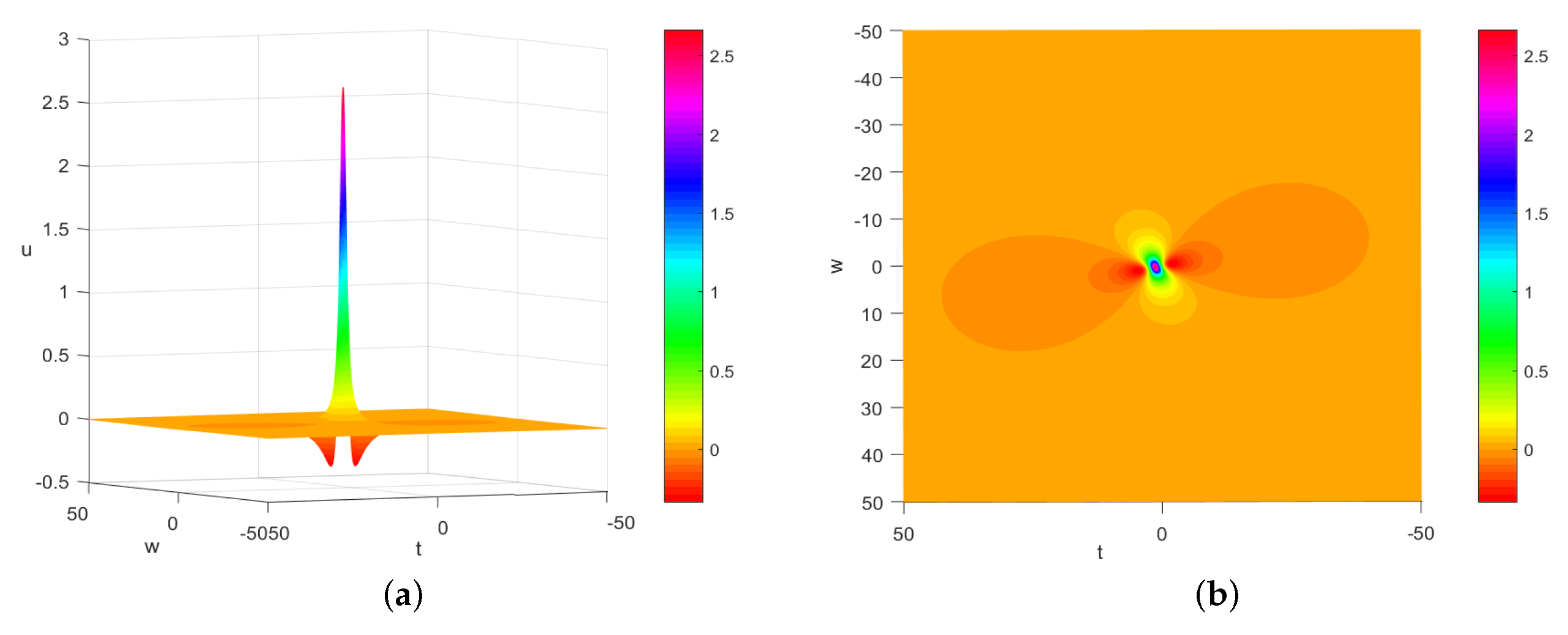
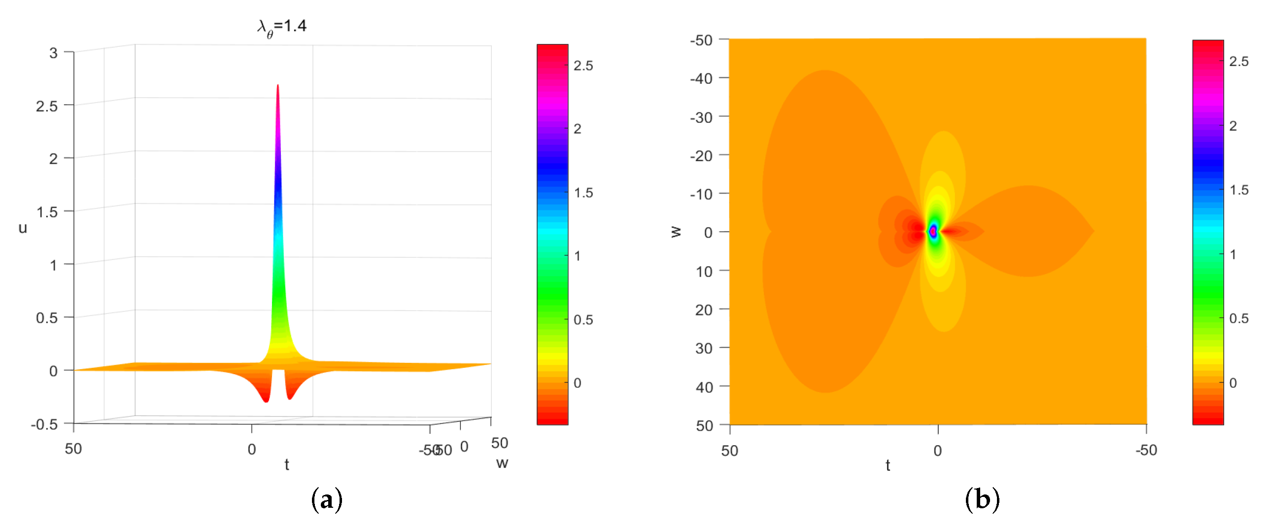
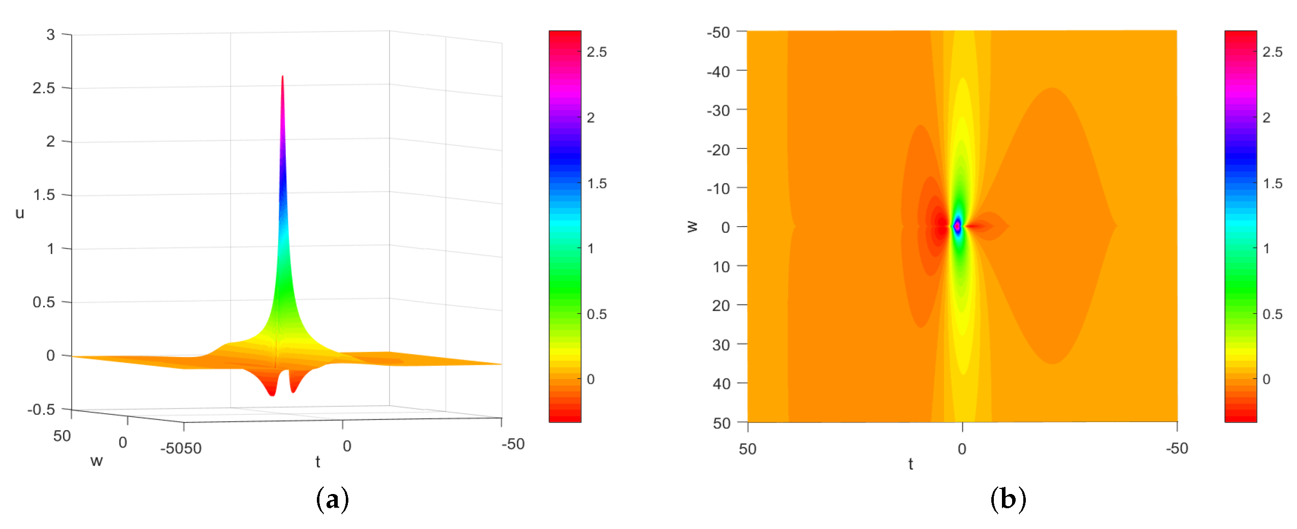
4.1. Rogue Wave Solutions of the (4 + 1)-Dimensional Time-Fractional Fokas Equation

First, let us introduce Hirota bilinear methods. The Hirota bilinear method’s main goal is to convert the equation into a bilinear form by using variable transformation and bilinear derivative to generate an auxiliary function, which can then be solved. Using fractional transformation and the bilinear approach, we investigate the rogue wave solution of the (4 + 1)-dimensional Fokas equation.
Definition 5.
The Hirota bilinear operator (d-operator) is defined as follows
D x n ( a , b ) x y n a ( x ) b ( y ) y = x = n y n a ( x + y ) b ( x y ) y = 0 , D t m D x n ( a , b ) m s m n y n a ( t + s , x + y ) b ( t s , x y ) s = 0 y = 0 .
According to the definition of Hirota bilinear operator, we can obtain
D x 2 ( f · f ) = 2 f x x f 2 f x 2 D x D t ( f · f ) = 2 f x t f 2 f x f t D x 4 ( f · f ) = 2 f x x x x f 8 f x x x f x + 6 f x x 2
For the (4 + 1)-dimensional time-fractional Fokas equation:
4 D t σ u x u x x x y + u x y y y + 12 u x u y + 12 u u x y 6 u z w = 0 .
At the same time, we perform fractional transformation:
T = m t σ Γ ( 1 + σ ) ,
where m is a constant. It can be obtained from the above equation
σ u t σ = m u T ,
Equation (39) can be written as
4 u T x u x x x y + u x y y y + 12 u x u y + 12 u u x y 6 u z w = 0 .
First, we take the following transformation:
ζ = α x + β y ,
where α and β are undetermined constants. Then, Equation (40) becomes
u T + 1 4 β β 2 α 2 u ζ ζ ζ + 3 2 β u 2 ζ ζ 3 2 u z w = 0 .
We introduce the following variable transformation
A = R ( ln f ) ζ ζ , R = β 2 α 2 .
Equation (39) can be transformed into bilinear form as follows:
D ζ D t + 1 4 β β 2 α 2 D ζ 4 3 2 α D z D w f · f = 0 .
According to Definition 5, the bilinear form Equation (44) can be expanded as
D ζ D t + 1 4 β β 2 α 2 D ζ 4 3 2 α D z D w f · f = f ζ T f f ζ f T + 1 4 β ( β 2 α 2 ) ( f ζ ζ ζ ζ f 4 f ζ ζ ζ f ζ 3 f ζ ζ 2 ) 3 2 α ( f z w f f z f w ) = 0 .
Let us assume that
f = ( m ( ζ , z , w , T ) ) 2 + ( n ( ζ , z , w , T ) ) 2 + ( l ( ζ , z , w , T ) ) 2 + b 13 , m ( ζ , z , w , T ) = b 1 ζ + b 2 z + b 3 w + b 4 T , n ( ζ , z , w , T ) = b 5 ζ + b 6 z + b 7 w + b 8 T , l ( ζ , z , w , T ) = b 9 ζ + b 10 z + b 11 w + b 12 T ,
where b i ( i = 1 , 2 , , 13 ) are real parameters to be determined.
Through calculation, we obtain the solution of the following parameters:
b 4 = 3 d 1 2 α d 4 , b 8 = 3 d 2 2 α d 4 , b 12 = 3 d 3 2 α d 4 , b 7 = b 3 ( b 3 b 10 b 6 b 9 ) + b 11 ( b 1 b 6 b 2 b 5 ) b 1 b 10 b 2 b 9 , b 13 = α β β 2 α 2 b 1 2 + b 9 2 + b 5 2 3 a 1 b 10 b 2 b 9 2 b 1 b 11 b 3 b 9 b 1 b 10 b 2 b 9 2 + b 5 b 10 b 6 b 9 2 + b 1 b 6 b 2 b 5 2 .
where
d 1 = b 3 b 2 b 9 b 1 b 10 b 1 b 2 + b 9 b 10 b 1 b 6 2 b 9 b 2 b 5 2 b 10 + 2 b 2 b 5 b 6 b 9 + b 11 b 1 b 10 b 2 b 9 2 + b 1 b 6 b 2 b 5 2 , d 2 = b 3 b 5 b 10 b 6 b 9 b 9 b 10 + b 5 b 6 + b 2 2 b 5 b 9 + b 1 2 b 6 b 10 2 b 1 b 2 b 6 b 9 + b 11 b 2 b 6 b 1 2 b 5 2 b 9 2 + b 1 b 5 b 6 2 b 2 2 b 10 2 + 2 b 1 b 6 b 9 b 10 , d 3 = b 3 b 1 b 10 b 2 b 9 2 + b 6 b 9 b 5 b 10 2 + b 11 b 1 b 9 b 10 2 b 2 2 b 6 2 + b 2 b 10 b 1 2 b 5 2 b 9 2 + 2 b 1 b 5 b 6 b 10 , d 4 = b 1 2 + b 5 2 + b 9 2 b 1 b 10 b 2 b 9 .
Given the particularity of f, we find the following conditions:
α β β 2 α 2 b 1 b 10 b 2 b 9 b 1 b 11 b 3 b 9 > 0 ,
with
a 1 a 11 a 3 a 9 0 .
By importing the calculated parameters into Equation (43), the solution of Equation (39) is obtained
u = 2 ( β 2 α 2 ) [ ( b 1 2 + b 5 2 + b 9 2 ) ( m 2 + n 2 + l 2 + b 13 ) 2 ( b 1 m + b 5 n + b 9 l ) 2 ] ( m 2 + n 2 + l 2 + b 13 ) 2 ,
when T = m t σ Γ ( 1 + σ ) , we obtain the fractional solution of the equation.
Based on the solution Equation (48) of the (4 + 1)-dimensional fractional Fokas equation obtained by the bilinear method, the phenomenon of rogue waves in higher dimensional higher-order Fokas model is studied.
By selecting appropriate parameters, the image of the (4 + 1)-dimensional time-fractional order Fokas equation when the order of the fractional order is equal to 1 is drawn, see Figure 1a,b. Rogue waves have the property of appearing in a particular space and time, taking on a local structure in time. It is also easy to see from the image that they have significant features: large amplitude, sharp crest, short duration.
In order to study the rogue wave phenomenon in the fractional model, we select parameters σ = 0.75 and σ = 0.5 to obtain the rogue wave image of the (4 + 1)-dimensional temporal fractional Fokas equation, as presented in Figure 2a,b and Figure 3a,b. We can clearly observe the rogue wave similar to that in Figure 1 in Figure 2 and Figure 3. From the three sets of images, we find that when the value of σ is reduced, the rogue wave’s fluctuation range is enlarged and its amplitude remains unchanged.

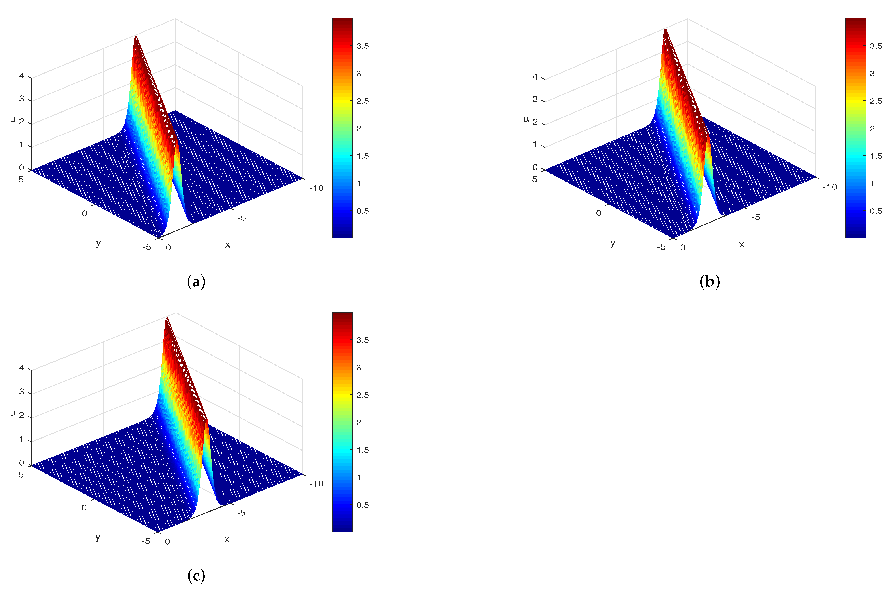
4.2. Multiple Soliton Solutions of the (4 + 1)-Dimensional Time-Fractional Fokas Equation

Based on the Hirota bilinear transformation introduced above, the multiple solution of Equation (39) is constructed by using Equation (44). First, we can suppose that there is a single soliton solution of Equation (39). Its form is
u ( ζ , z , w , T ) = R ( ln f ) ζ ζ , R = β 2 α 2 ,
where the auxiliary function f ( ζ , z , w , T ) is calculated by
f ( ζ , z , w , T ) = 1 + e ρ 1 ( ζ , z , w , T ) = 1 + e r 1 c 1 ζ + p 1 z + q 1 w 1 4 β ( β 2 α 2 ) c 1 4 r 1 2 3 p 1 q 1 2 c 1 α T ,
and c 1 , p 1 , q 1 are constant.
Thus, the soliton solution of the (4 + 1)-dimensional Fokas equation is
u ( ζ , z , w , T ) = ( β 2 α 2 ) ln ( 1 + e ρ 1 ) ζ ζ = 1 4 r 1 2 ( β 2 α 2 ) s e c h 2 ρ 1 2 ,
where
ρ 1 = r 1 c 1 ζ + p 1 z + q 1 w 1 4 β ( β 2 α 2 ) c 1 4 r 1 2 3 p 1 q 1 2 c 1 α T .
Then, the soliton solution of the (4 + 1)-dimensional time-fractional Fokas equation is:
u ( ζ , z , w , t ) = ( β 2 α 2 ) ln ( 1 + e ρ 1 ) ζ ζ = 1 4 r 1 2 ( β 2 α 2 ) s e c h 2 r 1 c 1 ζ + p 1 z + q 1 w 1 4 β ( β 2 α 2 ) c 1 4 r 1 2 3 p 1 q 1 2 c 1 α t σ Γ ( 1 + σ ) 2 .
Assuming ζ = 3 x + 5 y , Figure 4a–c obtain isolated wave motion images with different T values under integer solutions. In order to study the soliton solution in the fractional model, we assume that σ = 0.2 , σ = 0.5 , σ = 0.8 at t = 2 to obtain the motion of the bell soliton in Figure 5.
We can see from the figure that the bell solitary wave is moving in the negative direction of the x-axis. Figure 5 illustrates the solution of the (4 + 1)-dimensional time-fractional Fokas model with similar wave form of integer order form. As σ increases, the bell wave moves along the negative X-axis. For the double-soliton solution, we suppose
f ( ζ , z , w , T ) = 1 + e ρ 1 + e ρ 2 + e ρ 1 + ρ 2 + A 12 .
According to Definition 5, we can obtain e A 12 in the above equation as:
e A 12 = α β β 2 α 2 r 2 r 1 2 + 2 p 2 p 1 q 2 q 1 α β β 2 α 2 r 2 + r 1 2 + 2 p 2 p 1 q 2 q 1 .
Substitute Equation (53) into
u = ( β 2 α 2 ) ( ln f ) ζ ζ
We obtain the two-soliton solution of (4 + 1)-dimensions Fokas as follows
u = ( β 2 α 2 ) [ ln ( 1 + e ρ 1 + e ρ 2 + e ρ 1 + ρ 2 + A 12 ) ] ζ ζ ,
where
ρ i ( ζ , z , w , T ) = r i { c i ζ + p i z + q i w + [ 1 4 β ( β 2 α 2 ) c i 4 r i 2 + 3 p i q i 2 α c i ] T } , i = 1 , 2 .
Then we obtain the two-soliton solution of the (4 + 1)-dimensional time-fractional Fokas equation.
u = ( β 2 α 2 ) [ ln ( 1 + e ρ 1 + e ρ 2 + e ρ 1 + ρ 2 + A 12 ) ] ζ ζ ; ρ i = r i { c i ζ + p i z + q i w + 1 4 β ( β 2 α 2 ) c i 4 r i 2 + 3 p i q i 2 α c i m t σ Γ ( 1 + σ ) } , i = 1 , 2 .
Next, we find the three-soliton solution. Assuming that
f = 1 + e ρ 1 + e ρ 2 + e ρ 3 + e ρ 1 + ρ 2 + A 12 + e ρ 1 + ρ 3 + A 13 + e ρ 2 + ρ 3 + A 23 + e ρ 1 + ρ 2 + ρ 3 + A 12 + A 13 + A 23 .
Substituting into Equation (54), the three-soliton solution of the (4 + 1)-dimensional time-fractional Fokas equation is obtained.
u = β 2 α 2 ln 1 + e ρ 1 + e ρ 2 + e ρ 3 + e ρ 1 + ρ 2 + A 12 + e ρ 1 + ρ 3 + A 13 + e ξ ρ 2 + ρ 3 + A 23 + e ρ 1 + ρ 2 + ρ 3 + A 12 + A 13 + A 23 ζ ζ ,
where
ρ i = r i c i ζ + p i z + q i w + 1 4 β ( β 2 α 2 ) c i 4 r i 2 + 3 p i q i 2 α c i m t σ Γ ( 1 + σ ) , i = 1 , 2 .
and
e A i j = α β β 2 α 2 r j r i 2 + 2 p j p i q j q i α β β 2 α 2 r j + r i 2 + 2 p j p i q j q i .
Similarly, we assume:
f n = μ = 0 , 1 e i = 1 n μ i ξ i + A 1 i < l n μ i μ j A i j ,
We can obtain the formula of n-soliton solution of the (4 + 1)-dimensional time-fractional Fokas equation:
u = β 2 α 2 ln μ = 0 , 1 e i = 1 n μ i ξ i + A 1 i < l n μ i μ j A i j ζ ζ ,
where i , j = 1 , 2 , , n .

5. The Numerical Solutions of the Time-Fractional Fokas Equation

Definition 6
([49]). The Riemann–Liouville fractional integral operator of order σ > 0 for a function ξ ( x ) is defined as
Φ α ξ ( x ) = 1 Γ ( σ ) 0 x ( x t ) σ 1 ξ ( t ) d t , σ > 0 , x > 0 ,
and some properties are given as follows:
Φ σ Φ ϱ ξ ( x ) = Φ ϱ Φ σ ξ ( x ) , Φ σ Φ ϱ ξ ( x ) = Φ α + ϱ ξ ( x ) , Φ σ x γ = Γ ( γ + 1 ) Γ ( σ + γ + 1 ) x σ + γ .
Lemma 1.
If u ( t ) C 2 [ 0 , T ] ,
I o + σ μ ( t k + 1 ) I o + σ μ ( t k ) = τ σ Γ ( γ + 1 ) [ μ ( t k + 1 ) + j = 0 k 1 ( ω j + 1 ω j ) μ ( t k j ) ] + R k , σ ,
in which
| R k , σ | C ω K τ 1 + σ , 1 = ϖ 0 > ϖ 1 > > ϖ k > 0 , ϖ j = ( j + 1 ) σ j σ .
Additionally, I 0 + σ μ ( t k ) is referred to as the Riemann–Liouville fractional integral of order σ.

5.1. Time Discretization

The time-fractional Fokas equation is regarded as
4 D t σ u x u x x x y + u x y y y + 12 u x u y + 12 u u x y 6 u z w = 0 , 0 < t T , ( x , y ) Ω .
After dimensionality reduction, the equation becomes
D t σ u ζ + 1 4 β ( β 2 α 2 ) u ζ ζ ζ ζ + 3 β 2 ( u 2 ) ζ ζ 3 2 α u z w = 0 ,
with the boundary condition being extracted from the exact solution given in Equation (52) as follows:
( ζ , z , w , t ) = h ( ζ , z , w , t ) = 1 4 r 1 2 ( β 2 α 2 ) s e c h 2 ( r 1 ( c 1 ζ + p 1 z + q 1 w ) ( 1 4 β ( β 2 α 2 ) c 1 4 r 1 2 3 p 1 q 1 2 c 1 α ) t σ Γ ( 1 + σ ) 2 ) ,
and the initial condition
u ( ζ , z , w , 0 ) = η ( ζ , z , w ) = 1 4 r 1 2 ( β 2 α 2 ) s e c h 2 ( r 1 ( k 1 ζ + p 1 z + q 1 w ) 2 ) ,
According to Lemma 5.1, Equation (66) becomes
I 0 + σ u ( ζ , z , w , t k + 1 ) x I 0 + σ u ( ζ , z , w , t k ) x + 1 4 β ( β 2 α 2 ) [ 4 u ( ζ , z , w , t k + 1 ) ζ ζ ζ ζ 4 u ( ζ , z , w , t k ) ζ ζ ζ ζ ] + 3 β 2 [ 2 u 2 ( ζ , z , w , t k + 1 ) ζ ζ 2 u 2 ( ζ , z , w , t k ) ζ ζ ] 3 2 α [ 2 u ( ζ , z , w , t k + 1 ) z w 2 u ( ζ , z , w , t k ) z w ] = 0 .
Then, we have
u k + 1 x + 1 μ [ 1 4 β ( β 2 α 2 ) 4 u k + 1 ζ ζ ζ ζ + 3 β 2 2 ( u k + 1 ) 2 ζ ζ 3 2 α 2 u k + 1 z w ] = 1 μ [ 1 4 β ( β 2 α 2 ) 4 u k ζ ζ ζ ζ + 3 β 2 2 ( u k ) 2 ζ ζ 3 2 α 2 u k z w ] j = 0 1 ( λ j + 1 λ j ) u k j x ,
in which
μ = τ σ Γ ( 1 + σ ) , λ j = ( j + 1 ) σ j σ .

5.2. Radial Basis Function Meshless Method

In R 2 , we assume that Ω is an arbitrary domain. The following are approximate expansion of u ( x i , y i , t n ) :
u ζ i , z i , w i , t n = j = 1 c j n Φ r i j ,
in which
φ r i j = ζ i ζ j 2 + z i z j 2 + w i w j 2 + c 2 = r 2 + c 2 .
We denote
Φ j ( ζ , z , w ) = ζ ζ j 2 + z z j 2 + w w j 2 + c 2 = r j 2 + c 2 ,
in which r j is the Euclidean norm given by r j = ζ ζ j + z z j + w w j and c is the shape parameter. According to Equation (70), for k = 0 , we can obtain
u 1 x + 1 μ [ 1 4 β ( β 2 α 2 ) 4 u 1 ζ ζ ζ ζ + 3 β 2 2 ( u 1 ) 2 ζ ζ 3 2 α 2 u 1 z w ] = 1 μ [ 1 4 β ( β 2 α 2 ) 4 u 0 ζ ζ ζ ζ + 3 β 2 2 ( u 0 ) 2 ζ ζ 3 2 α 2 u 0 z w ] ,
and for 1 k N 1 , we have
u k + 1 x + 1 μ [ 1 4 β ( β 2 α 2 ) 4 u k + 1 ζ ζ ζ ζ + 3 β 2 2 ( u k + 1 ) 2 ζ ζ 3 2 α 2 u k + 1 z w ] = 1 μ [ 1 4 β ( β 2 α 2 ) 4 u k ζ ζ ζ ζ + 3 β 2 2 ( u k ) 2 ζ ζ 3 2 α 2 u k z w ] j = 0 1 ( λ j + 1 λ j ) u k j x .
Now, substituting Equation (73) into Equations (76) and (77), we can obtain the following matrix in the following format:
Qc k + 1 = P k + 1 , k = 0 , 1 , , N + 1 ,
where
Q = Φ r 1 , 1 Φ r 1 , 2 Φ r 1 , n + 1 Φ r 1 , N Φ r 2 , 1 Φ r 2 , 2 Φ r 2 , n + 1 Φ r 2 , N Φ r n , 1 Φ r n , 2 Φ r n , n + 1 Φ r n , N L Φ r n + 1 , 1 L Φ r n + 1 , 2 L Φ r n + 1 , n + 1 L Φ r n + 1 , N L Φ r N , 1 L Φ r N , 2 L Φ r N , n + 1 L Φ r N , N ,
L Φ r i j = Φ j ( ζ j , z j , w j ) ζ + 1 μ [ 1 4 β ( β 2 α 2 ) 4 Φ j ( ζ j , z j , w j ) ζ 4 + 3 β 2 2 ( Φ j ( ζ j , z j , w j ) ) 2 ζ 2 3 2 α 2 Φ j ( ζ j , z j , w j ) z w ] | ( ζ , z , w ) = ( ζ i , z i , w i ) ,
n + 1 i N , 1 j N 1 , c k + 1 = c 1 k + 1 , c 2 k + 1 , , c N k + 1 T , P k + 1 = p 1 k + 1 , p 2 k + 1 , , p N k + 1 ,
in which
p i 1 = η ( ζ , z , w ) | ( ζ , z , w ) = ( ζ i , z i , w i ) , n + 1 i N ,
and also
p i k + 1 = 1 μ [ 1 4 β ( β 2 α 2 ) 4 Φ ( r i j ) ζ 4 + 3 β 2 2 ( Φ ( r i j ) ) 2 ζ 2 3 2 α 2 Φ ( r i j ) z w ] j = 0 1 ( λ j + 1 λ j ) Φ ( r i j ) x
n + 1 i N , 1 k N 1 ,
b i k + 1 = h ( ζ , z , w ) | ( ζ , z , w ) = ( ζ i , z i , w i ) , 1 i n , 1 k N 1 .

5.3. Discussion of the Solutions

We use the numerical solution obtained by the RBF method and the exact solution obtained by the bilinear method. Next, we will discuss the absolute error of the two solutions. To ensure the method’s correctness, we took the absolute errors when σ = 0.75 , σ = 0.5 and σ = 1 respectively, as shown in Table 1, Table 2 and Table 3. When σ = 1 , it indicates that it is in the integer order. The numerical results of the time-fractional Fokas equation determined using the RBF approach are correct, as shown in the table.
By comparing the absolute errors of two solutions generated by the RBF method and the bilinear method, the accuracy of the RBF method may be determined. Furthermore, the numerical findings show that the RBF method suggested above yields a high-precision numerical solution to the fractional differential Fokas problem.
The accuracy of the RBF approach can be measured by comparing the absolute errors of two solutions given by the RBF method and the bilinear method. Furthermore, the numerical results demonstrate that the RBF method proposed above offers a high-precision numerical solution to the fractional differential Fokas issue.

6. Conclusions

In this paper, we first derived the (4 + 1)-dimensional time-fractional Fokas equation by using the semi-inverse method and fractional variational principle, and discussed the conservation law of the time-fractional Fokas equation by using the Lie symmetry analysis method. Then the rogue wave solutions and soliton solutions of (4 + 1)-dimensional time-fractional Fokas equation were obtained by using bilinear approach. Finally, the numerical solution of the (4 + 1)-dimensional time-fractional order Fokas equation was obtained by using the Radial Basis Function (RBF) meshless method, and the absolute error analysis under different conditions was given. The work in this paper promotes the research of high-dimensional integrable systems. The precise numerical solutions of the high-dimensional fractional model we have obtained are of great significance to the study of physical phenomena in real life.

Author Contributions

Writing—original draft preparation, Z.J.; writing—review and editing, Z.-G.Z.; visualization, J.-J.L.; supervision, H.-W.Y. All authors have read and agreed to the published version of the manuscript.

Funding

This research was supported by National Natural Science Foundation of China (No. 11975143).

Institutional Review Board Statement

Not applicable.

Informed Consent Statement

Not applicable.

Data Availability Statement

Not applicable.

Conflicts of Interest

The authors declare no conflict of interest.

References

  1. Benkhettou, N.; Hassani, S.; Torres, D.F.M. A conformable fractional calculus on arbitrary time scales. J. King Saud Univ. Sci. 2016, 28, 93–98. [Google Scholar] [CrossRef]
  2. Lokenath, D. Recent applications of fractional calculus to science and engineering. Int. J. Math. Math. Sci. 2014, 2003, 3413–3442. [Google Scholar]
  3. Gorenflo, R.; Mainardi, F. Fractional Calculus: Integral and Differential Equations of Fractional Order. Mathematics 2008, 49, 277–290. [Google Scholar]
  4. Miller, K.S.; Ross, B. An introduction to the fractional calculus and fractional differential equations. Wiley 1993, 126–174. [Google Scholar]
  5. Agarwal, R.P.; Benchohra, M.; Hamani, S. A Survey on Existence Results for Boundary Value Problems of Nonlinear Fractional Differential Equations and Inclusions. Acta Appl. Math. 2010, 109, 973–1033. [Google Scholar] [CrossRef]
  6. Sakar, M.G.; Uludag, F.; Erdogan, F. Numerical solution of time-fractional nonlinear PDEs with proportional delays by homotopy perturbation method. Appl. Math. Model. 2016, 40, 6639–6649. [Google Scholar] [CrossRef]
  7. Hosseini, S.M.; Asgari, Z. Solution of stochastic nonlinear time fractional PDEs using polynomial chaos expansion combined with an exponential integrator. Comput. Math. Appl. 2016, 73, 997–1007. [Google Scholar] [CrossRef]
  8. Hosseini, K.; Ma, W.X.; Ansari, R.; Mirzazadeh, M.; Pouyanmehr, R.; Samadani, F. Evolutionary behavior of rational wave solutions to the (4 + 1)- dimensional Boiti-Leon-Manna-Pempinelli equation. Phys. Scr. 2020, 95, 065208. [Google Scholar] [CrossRef]
  9. Fokas, A.S. Integrable nonlinear evolution partial differential equations in 4 + 2 and 3 + 1 dimensions. Phys. Rev. Lett. 2006, 96, 190201. [Google Scholar] [CrossRef]
  10. Ohta, Y.; Yang, J. Rogue waves in the Davey-Stewartson I equation. Phys. Rev. E Stat. Nonlin. Soft Matter. Phys. 2012, 86, 694–698. [Google Scholar] [CrossRef] [Green Version]
  11. Jafari, H.; Kadem, A.; Baleanu, D.; Yilmaz, T. Solutions of the fractional Davey-Stewartson equations with variational iteration method. Rom. Rep. Phys. 2012, 64, 337–346. [Google Scholar]
  12. Ying, Z.; Xie, F.; Lv, Z. Symbolic computation in non-linear evolution equation: Application to (3 + 1)-dimensional Kadomtsev-Petviashvili equation. Chaos Solitons Fractals 2005, 24, 257–263. [Google Scholar]
  13. Bi, Y.; Zhang, Z.; Liu, Q.; Liu, T. Research on nonlinear waves of blood flflow in arterial vessels. Commun. Nonlinear Sci. Numer. Simul. 2021, 102, 105918. [Google Scholar] [CrossRef]
  14. Yang, Y.; Song, J. On the generalized eigenvalue problem of Rossby waves vertical velocity under the condition of zonal mean flow and topography. Appl. Math. Lett. 2021, 121, 107485. [Google Scholar] [CrossRef]
  15. El-Ganaini, S.; Al-Amr, M.O. New abundant wave solutions of the conformable space-time fractional (4 + 1)-dimensional Fokas equation in water waves. Comput. Math. Appl. 2019, 78, 2094–2106. [Google Scholar] [CrossRef]
  16. Zhang, S.; Zhang, H. Fractional sub-equation method and its applications to nonlinear fractional PDEs. Phys. Lett. A 2011, 375, 1069–1073. [Google Scholar] [CrossRef]
  17. He, J.H. Application of homotopy perturbation method to nonlinear wave equations. Chaos Solitons Fractals 2005, 26, 695–700. [Google Scholar] [CrossRef]
  18. He, J.H.; Wu, X.H. Exp-function method for nonlinear wave equations. Chaos Solitons Fractals 2006, 30, 700–708. [Google Scholar] [CrossRef]
  19. Ramos, J.I. On the variational iteration method and other iterative techniques for nonlinear differential equations. Appl. Math. Comput. 2008, 199, 39–69. [Google Scholar] [CrossRef]
  20. Demiray, S.T.; Bulut, H. A New Method for (4 + 1)-Dimensional Fokas Equation. ITM Web Conf. 2008, 22, 01065. [Google Scholar] [CrossRef]
  21. He, Y. Exact Solutions for-Dimensional Nonlinear Fokas Equation Using Extended F-Expansion Method and Its Variant. Math. Probl. Eng. 2014, 2014, 972519. [Google Scholar]
  22. Lee, J.; Sakthivel, R.; Wazzan, L. Exact travelling wave solutions of a higher-dimensions of a higher-dimensional nonlinear evolution equation. Mod. Phys. Lett. B 2010, 24, 1011–1021. [Google Scholar] [CrossRef]
  23. Wazwaz, A.M. Multiple-soliton solutions for the KP equation by Hirota’s bilinear method and by the tanh-coth method. Appl. Math. Comput. 2007, 190, 633–640. [Google Scholar] [CrossRef]
  24. Tian, H.F.; Ha, J.T.; Zhang, H.Q. Lump-type solutions, interaction solutions and periodic wave solutions of a (3 + 1)-dimensional Korteweg-de Vries equation. Int. J. Mod. Phys. B 2019, 33, 1950319. [Google Scholar] [CrossRef]
  25. Tajiri, M.; Takeuchi, K.; Arai, T. Soliton Stability to the Davey-Stewartson I Equation by the Hirota Method. J. Phys. Soc. Jpn. 2001, 70, 1505–1511. [Google Scholar] [CrossRef]
  26. Zhang, S.; Liu, D. Multisoliton solutions of a (2 + 1)-dimensional variable-coefficient Toda lattice equation via Hirota’s bilinear method. Can. J. Phys. 2014, 92, 184–190. [Google Scholar] [CrossRef]
  27. Dong, M.J.; Tian, S.F.; Yan, X.W.; Zou, L. Solitary waves, homoclinic breather waves and rogue waves of the (3 + 1)-dimensional Hirota bilinear equation. Comput. Math. Appl. 2018, 75, 957–964. [Google Scholar] [CrossRef]
  28. Feng, B.F. General N-soliton solution to a vector nonlinear Schrödinger equation. J. Phys. A Math. Theor. 2014, 47, 355203. [Google Scholar] [CrossRef]
  29. Wang, D.S.; Zhang, Y.; Dong, H.H. Riemann-Hilbert problems and soliton solutions for a multi-component cubic-quintic nonlinear Schrödinger equation. J. Geom. Phys. 2020, 149, 103569. [Google Scholar]
  30. Ohta, Y.; Yang, J. General high-order rogue waves and their dynamics in the nonlinear Schrodinger equation. Proc. R. Soc. Math. Phys. Eng. Sci. 2012, 468, 1716–1740. [Google Scholar] [CrossRef] [Green Version]
  31. Wang, L.H.; Porsezian, K.; He, J.S. Breather and rogue wave solutions of a generalized nonlinear Schrödinger equation. Phys. Rev. E 2013, 87, 053202. [Google Scholar] [CrossRef] [PubMed] [Green Version]
  32. Lv, Z.S.; Zhang, H.Q. Soliton-like and period form solutions for high dimensional nonlinear evolution equations. Solitons Fractals 2003, 17, 669–673. [Google Scholar]
  33. Zhu, X.G.; Nie, Y.F.; Wang, J.G.; Yuan, Z.B. An advanced meshless approach for the high-dimensional multi-term time-space-fractional PDEs on convex domains. Nonlinear Dyn. 2021, 104, 1555–1580. [Google Scholar] [CrossRef]
  34. Chenoweth, M.E. A Local Radial Basis Function Method for the Numerical Solution of Partial Differential Equations. Master’s Thesis, Marshall University, Huntington, WV, USA, 2012. [Google Scholar]
  35. Khalique, C.M.; Adem, A.R. Symmetry reductions, exact solutions and conservation laws of a new coupled KdV system. Commun. Nonlinear Sci. Numer. Simul. 2012, 17, 3465–3475. [Google Scholar]
  36. Leo, R.A.; Sicuro, G.; Tempesta, P. A foundational approach to the Lie theory for fractional order partial differential equations. Fract. Calc. Appl. Anal. 2017, 20, 212. [Google Scholar] [CrossRef] [Green Version]
  37. Kinani, E.E.; Ouhadan, A. Lie symmetry analysis of some time fractional partial differential equations. Int. J. Mod. Phys. Conf. 2015, 38, 1560075. [Google Scholar] [CrossRef] [Green Version]
  38. Treanţă, S. Gradient Structures Associated with a Polynomial Differential Equation. Mathematics 2020, 8, 535. [Google Scholar] [CrossRef] [Green Version]
  39. Lie, S. Theorie der Transformationsgruppen I. Christiania 1880, 16, 441–528. [Google Scholar] [CrossRef]
  40. Sun, J.C.; Zhang, Z.G.; Dong, H.H.; Yang, H.W. Dust acoustic rogue waves of fractional-order model in dusty plasma. Commun. Theor. Phys. 2020, 72, 17. [Google Scholar] [CrossRef]
  41. Gazizov, R.K.; Kasatkin, A.A.; Lukashchuk, S.Y. Continuous transformation groups of fractional differential equations. Vestn. Usatu 2007, 9, 21. [Google Scholar]
  42. Sabatier, J.; Agrawal, O.P.; Machado, J. Advances in Fractional Calculus. Fract. Var. Princ. 2007, 115–126. [Google Scholar]
  43. He, J.H.; Wu, G.C.; Austin, F. The Variational Iteration Method Which Should Be Followed. Nonl. Sci. Lett. A 2010, 1, 1–30. [Google Scholar]
  44. Saxena, R.; Mathai, A.; Haubold, H. Space-time fractional reaction-diffusion equations associated with a generalized Riemann-Liouville fractional derivative. Axioms 2014, 3, 320–334. [Google Scholar] [CrossRef] [Green Version]
  45. Treanţă, S. Noether-Type First Integrals Associated with Autonomous Second-Order Lagrangians. Symmetru 2019, 11, 1088. [Google Scholar] [CrossRef] [Green Version]
  46. He, J.H. A tutorial and heuristic review on Lagrange multiplier for optimal problems. Nonlinear Sci. Lett. A 2017, 8, 121–148. [Google Scholar]
  47. Hu, J.; Ye, Y.; Shen, S.; Zhang, J. Lie symmetry analysis of the time fractional KdV-type equation. Appl. Math. Comput. 2014, 233, 439–444. [Google Scholar] [CrossRef]
  48. Saberi, E.; Hejazi, S.R. Lie symmetry analysis, conservation laws and exact solutions of the time-fractional generalized Hirota-Satsuma coupled KdV system. Phys. A Stat. Mech. Its Appl. 2018, 492, 296–307. [Google Scholar] [CrossRef]
  49. Agarwal, P.; Tariboon, J.; Ntouyas, S.K. Some generalized Riemann-Liouville k-fractional integral inequalities. J. Inequalities Appl. 2016, 2016, 122. [Google Scholar] [CrossRef] [Green Version]
Figure 1. Evolution plots of Equation (48) by choosing α = 2 , β = 4 , a 1 = 1 , a 2 = 1 , a 3 = 2 , a 5 = 1 , a 6 = 0 , a 9 = 1 , a 10 = 1 , a 11 = 1 . (a) σ = 1 ; (b) σ = 1 .
Fractalfract 06 00108 g001
Figure 2. Evolution plots of Equation (48) by choosing α = 2 , β = 4 , a 1 = 1 , a 2 = 1 , a 3 = 2 , a 5 = 1 , a 6 = 0 , a 9 = 1 , a 10 = 1 , a 11 = 1 . (a) σ = 0.75 ; (b) σ = 0.75 .
Fractalfract 06 00108 g002
Figure 3. Evolution plots of Equation (48) by choosing α = 2 , β = 4 , a 1 = 1 , a 2 = 1 , a 3 = 2 , a 5 = 1 , a 6 = 0 , a 9 = 1 , a 10 = 1 , a 11 = 1 . (a) σ = 0.5 ; (b) σ = 0.5 .
Fractalfract 06 00108 g003
Figure 4. In the case of integer order solution, evolution plots of single soliton solution created by choosing c 1 = 1 , r 1 = 1 , α = 3 , β = 5 , p 1 = 2 , q 1 = 3 , z = 0 , w = 0 . (a) T = 1 ; (b) T = 0 ; (c) T = 1 .
Fractalfract 06 00108 g004
Figure 5. In the case of fractional solution, evolution plots of single soliton solution by choosing c 1 = 1 , r 1 = 1 , α = 3 , β = 5 , p 1 = 2 , q 1 = 3 , z = 0 , w = 0 . (a) t = 2 , σ = 0.2 ; (b) t = 2 , σ = 0.5 ; (c) t = 2 , σ = 0.8 .
Fractalfract 06 00108 g005
Table 1. The absolute errors obtained by the radial basis function method with regard to exact solution obtained by the bilinear method for (4 + 1)-dimensional Fokas equation given in Equation (13) at different points of ζ and t taking σ = 0.75 ; α = 1 ; β = 2 ; r 1 = 2 ; c 1 = 1 ; p 1 = 1 ; q 1 = 2 ; τ = 1 / 80 ; c = 1 .
u RBF ( MQ ) u Exact
ζ t = 0.1t = 0.2t = 0.3t = 0.4t = 0.5t = 0.6t = 0.7t = 0.8t = 0.9t = 1
0.14.17 × 10 2 1.11 × 10 1 1.51 × 10 1 1.63 × 10 1 1.50 × 10 1 1.16 × 10 1 6.65 × 10 2 1.01 × 10 2 4.48 × 10 2 8.95 × 10 2
0.21.75 × 10 2 6.93 × 10 2 1.06 × 10 1 1.28 × 10 1 1.40 × 10 1 1.43 × 10 1 1.40 × 10 1 1.34 × 10 1 1.31 × 10 1 1.34 × 10 1
0.36.50 × 10 3 3.07 × 10 2 4.53 × 10 2 5.37 × 10 2 5.96 × 10 2 6.65 × 10 2 7.81 × 10 2 9.78 × 10 2 1.29 × 10 1 1.73 × 10 1
0.49.50 × 10 3 1.60 × 10 2 1.51 × 10 2 1.03 × 10 2 5.13 × 10 3 3.65 × 10 3 1.01 × 10 2 2.87 × 10 2 6.36 × 10 2 1.18 × 10 1
0.58.60 × 10 3 1.04 × 10 2 5.83 × 10 3 2.44 × 10 3 1.17 × 10 2 1.87 × 10 2 1.97 × 10 2 1.02 × 10 2 1.43 × 10 2 5.82 × 10 2
0.67.40 × 10 3 2.19 × 10 4 2.16 × 10 3 3.05 × 10 4 5.74 × 10 3 1.21 × 10 2 1.65 × 10 2 1.50 × 10 2 3.06 × 10 3 2.43 × 10 2
0.74.22 × 10 2 2.15 × 10 2 6.35 × 10 3 2.96 × 10 3 6.49 × 10 3 5.06 × 10 3 6.45 × 10 4 3.41 × 10 3 2.63 × 10 3 8.12 × 10 3
0.89.53 × 10 2 5.73 × 10 2 2.57 × 10 2 1.99 × 10 3 1.24 × 10 2 1.74 × 10 2 1.41 × 10 2 5.46 × 10 3 4.00 × 10 3 8.87 × 10 3
0.91.64 × 10 1 1.08 × 10 1 5.92 × 10 2 2.13 × 10 2 3.29 × 10 3 1.36 × 10 2 1.05 × 10 2 3.39 × 10 3 2.33 × 10 2 4.34 × 10 2
12.47 × 10 1 1.73 × 10 1 1.09 × 10 1 5.93 × 10 2 2.70 × 10 2 1.38 × 10 2 1.91 × 10 2 3.99 × 10 2 7.14 × 10 2 1.07 × 10 1
Table 2. The absolute errors obtained by the radial basis function method with regard to exact solution obtained by the bilinear method for (4 + 1)-dimensional Fokas equation given in Equation (13) at different points of ζ and t taking σ = 0.5 ; α = 1 ; β = 2 ; r 1 = 2 ; c 1 = 1 ; p 1 = 1 ; q 1 = 2 ; τ = 1 / 80 ; c = 1 .
u RBF ( MQ ) u Exact
ζ t = 0.1t = 0.2t = 0.3t = 0.4t = 0.5t = 0.6t = 0.7t = 0.8t = 0.9t = 1
0.12.18 × 10 1 1.49 × 10 1 9.79 × 10 2 6.20 × 10 2 3.85 × 10 2 2.42 × 10 2 1.58 × 10 2 9.66 × 10 3 2.37 × 10 3 9.43 × 10 3
0.21.86 × 10 1 1.58 × 10 1 1.43 × 10 1 1.37 × 10 1 1.36 × 10 1 1.34 × 10 1 1.26 × 10 1 1.08 × 10 1 7.54 × 10 2 2.57 × 10 2
0.31.13 × 10 1 1.09 × 10 1 1.16 × 10 1 1.30 × 10 1 1.47 × 10 1 1.62 × 10 1 1.68 × 10 1 1.62 × 10 1 1.38 × 10 1 9.23 × 10 2
0.45.37 × 10 2 5.94 × 10 2 7.44 × 10 2 9.52 × 10 2 1.18 × 10 1 1.39 × 10 1 1.53 × 10 1 1.57 × 10 1 1.44 × 10 1 1.11 × 10 1
0.52.39 × 10 2 2.87 × 10 2 4.09 × 10 2 5.80 × 10 2 7.76 × 10 2 9.67 × 10 2 1.12 × 10 1 1.19 × 10 1 1.14 × 10 1 9.27 × 10 2
0.62.43 × 10 2 2.03 × 10 2 2.24 × 10 2 2.92 × 10 2 3.97 × 10 2 5.21 × 10 2 6.39 × 10 2 7.21 × 10 2 7.27 × 10 2 6.14 × 10 2
0.75.06 × 10 2 3.26 × 10 2 1.99 × 10 2 1.29 × 10 2 1.15 × 10 2 1.54 × 10 2 2.28 × 10 2 3.13 × 10 2 3.70 × 10 2 3.56 × 10 2
0.89.69 × 10 2 6.19 × 10 2 3.26 × 10 2 1.07 × 10 2 2.57 × 10 3 6.74 × 10 3 2.66 × 10 3 7.30 × 10 3 1.94 × 10 2 2.89 × 10 2
0.91.57 × 10 1 1.05 × 10 1 5.93 × 10 2 2.36 × 10 2 2.56 × 10 4 9.63 × 10 3 6.49 × 10 3 7.35 × 10 3 2.79 × 10 2 5.00 × 10 2
12.28 × 10 1 1.59 × 10 1 9.90 × 10 2 5.24 × 10 2 2.21 × 10 2 9.84 × 10 3 1.52 × 10 2 3.58 × 10 2 6.72 × 10 2 1.03 × 10 1
Table 3. The absolute errors obtained by radial basis function method with regard to exact solution obtained by the bilinear method for (4 + 1)-dimensional Fokas equation given in Equation (13) at different points of ζ and t taking σ = 1 ; α = 1 ; β = 2 ; r 1 = 2 ; c 1 = 1 ; p 1 = 1 ; q 1 = 2 ; τ = 1 / 80 ; c = 1 .
u RBF ( MQ ) u Exact
ζ t = 0.1t = 0.2t = 0.3t = 0.4t = 0.5t = 0.6t = 0.7t = 0.8t = 0.9t = 1
0.13.86 × 10 2 8.85 × 10 2 1.09 × 10 1 1.05 × 10 1 8.04 × 10 2 4.48 × 10 2 9.08 × 10 3 1.42 × 10 2 1.21 × 10 2 2.78 × 10 2
0.25.36 × 10 2 9.70 × 10 2 1.19 × 10 1 1.22 × 10 1 1.08 × 10 1 8.30 × 10 2 5.52 × 10 2 3.47 × 10 2 3.30 × 10 2 6.20 × 10 2
0.32.75 × 10 2 5.40 × 10 2 6.82 × 10 2 7.22 × 10 2 6.87 × 10 2 6.16 × 10 2 5.62 × 10 2 5.95 × 10 2 7.94 × 10 2 1.25 × 10 1
0.48.43 × 10 3 1.70 × 10 2 1.75 × 10 2 1.31 × 10 2 7.59 × 10 3 5.24 × 10 3 1.14 × 10 2 3.20 × 10 2 7.35 × 10 2 1.42 × 10 1
0.56.02 × 10 3 6.82 × 10 3 1.13 × 10 4 1.16 × 10 2 2.40 × 10 2 3.22 × 10 2 3.05 × 10 2 1.18 × 10 2 3.11 × 10 2 1.05 × 10 1
0.64.23 × 10 3 1.16 × 10 2 9.64 × 10 3 5.15 × 10 4 1.30 × 10 2 2.66 × 10 2 3.44 × 10 2 2.90 × 10 2 2.03 × 10 3 5.49 × 10 2
0.72.00 × 10 2 6.26 × 10 3 2.12 × 10 2 2.52 × 10 2 1.96 × 10 2 7.32 × 10 3 6.44 × 10 3 1.45 × 10 2 8.14 × 10 3 2.21 × 10 2
0.88.74 × 10 2 3.40 × 10 2 5.72 × 10 3 3.05 × 10 2 4.00 × 10 2 3.59 × 10 2 2.21 × 10 2 5.28 × 10 3 5.84 × 10 3 1.40 × 10 3
0.92.14 × 10 1 1.30 × 10 1 6.14 × 10 2 1.22 × 10 2 1.62 × 10 2 2.41 × 10 2 1.46 × 10 2 6.12 × 10 3 2.97 × 10 2 4.60 × 10 2
14.11 × 10 1 2.96 × 10 1 1.99 × 10 1 1.25 × 10 1 7.76 × 10 2 5.65 × 10 2 5.94 × 10 2 8.10 × 10 2 1.13 × 10 1 1.44 × 10 1
Publisher’s Note: MDPI stays neutral with regard to jurisdictional claims in published maps and institutional affiliations.

