
Fractal Analysis of Local Activity and Chaotic Motion in Nonlinear Nonplanar Vibrations for Cantilever Beams

1
Faculty of Science, Beijing University of Technology, Beijing 100124, China
2
School of Energy and Power, Beihang University, Beijing 100191, China
*
Author to whom correspondence should be addressed.
Fractal Fract. 2022, 6(4), 181; https://doi.org/10.3390/fractalfract6040181
Submission received: 21 February 2022
/
Revised: 21 March 2022
/
Accepted: 22 March 2022
/
Published: 24 March 2022
(This article belongs to the Special Issue Fractional Dynamical Systems: Applications and Theoretical Results)
Abstract
:Many problems in practical engineering can be simplified as the cantilever beam model, which is generally studied by theoretical analysis, experiment, and numerical simulation. This paper discusses the local activity of the nonlinear nonplanar motion of a cantilever beam at the equilibrium point. Firstly, the equilibrium point of the model and the Jacobian matrix have been calculated. The stability of the characteristic root corresponding to the characteristic polynomial has been analyzed. Secondly, the corresponding complexity function of the model at the equilibrium point has been given. Then, the local activity region of the model at the equilibrium point can be obtained by using the theory of the local activity. Based on the actual engineering research background, the damping coefficient is generally taken as 0 < c < 1. The cantilever beam model is the local activity at the equilibrium point only if the parameters of the model satisfy a certain condition. In the numerical simulation, it is found that when the proper parameters are selected in the local activity region, the cantilever beam can exhibit different types of chaotic motion. The local activity theory provides a theoretical basis for the parameter selection of the chaotic motion in the cantilever beam.
1. Introduction
Many engineering problems can be simplified to cantilever beam models, such as satellite antennas, piezoelectric energy harvesters [1], engine blades [2,3]. With the development of science and technology, modern engineering structures have developed in the direction of large, high-speed, light structures. Therefore, it is of great significance to study the nonlinear dynamic properties of cantilever beams.
The research on the nonlinear nonplanar motion of the cantilever beam mainly focuses on the analysis of complex nonlinear dynamic characteristics and the control of vibration and chaos of the cantilever beam. Nayfeh and Pai [4] used the Galerkin method and multiscale method to analyze the nonlinear planar and nonplanar vibration responses of non-elongated cantilever beams. It was found that the geometric nonlinearity has hard characteristics, which is the main factor of nonplanar response. They [5] utilized two nonlinear coupled integral differential equations to study the nonplanar response of a cantilever beam subjected to harmonic forced excitation. Dwivedy and Kar [6] applied multiscale method to analyze periodic and chaotic responses of a cantilever beam under parametric excitation with a mass block. Young and Juan [7] exploited Ritz Galerkin method to discretize the governing equation to study the nonlinear response of a fluttering cantilever beam subjected to random loads at the free end. Ma et al. [8] employed the finite element method to analyze dynamic characteristics of a cantilever beam with oblique cracks. Anderson et al. [9] studied the response of the cantilever beam from both theoretical and experimental aspects. The responses of the first, third, and fourth modes are also observed. Some results of the nonlinear dynamics [10,11] of thin flexible cantilever beams with rectangular cross sections are given by Cusumano and Moon Arafat et al. [12]. They studied the nonlinear nonplanar response of the non-elongated metal cantilever beam under parametric excitations, in which bifurcations and chaotic motions were found. Yao and Zhang et al. [13] studied the multi-pulse Shilnikov orbit and chaotic dynamics of the nonlinear nonplanar oscillation of the cantilever beam. Yao [14] took an extended Melnikov method in the resonant case to investigate the multi-pulse global bifurcations and chaotic dynamics of the high-dimension nonlinear system for a laminated composite piezoelectric rectangular plate. Yao and Niu [15] established a rotating pre-twisted cylindrical shell model with a presetting angle to investigate nonlinear dynamic responses of the aero-engine compressor blade, and found the nonlinear steady-state response through numerical simulations. Yao et al. [16] studied the nonlinear dynamic response of rotating blades with variable speed under high-temperature supersonic gas flow, which considered the change of rotating speed and the influence of centrifugal force. Dick et al. [17] investigated the dynamic behavior of cantilever beam-impactor systems at macro and micro scales numerically and experimentally. Yu et al. [18] studied the nonlinear dynamic response of an inner cantilever beam system by establishing a nonlinear dynamic model, which obtained the numerical solution of the exact governing equation by the shooting method. Francesco [19] studied the random bending vibration of a small-scale Bernoulli-Euler beam with external damping using a stress-driven nonlocal mechanics method. The damping effect between the beam and surrounding environment is simulated, and the closed expressions of power spectral density, correlation function, stationary variance, and non-stationary variance of displacement field are obtained.
It can be seen that theoretical analysis, numerical simulations, or experiments are generally used to study nonlinear nonplanar cantilever beams. In the process of numerical simulations and experiments, the phenomena of the period, quasi-periodicity, and chaos are observed by adjusting parameters, but whether the selection of parameters follows certain rules or not. That is to say, if the parameters satisfy certain conditions in numerical simulations, the nonlinear dynamic system is more likely to appear complexity phenomenon.
The passivity theory is widely used to analyze the stability of dynamical systems [20], and is a powerful tool to analyze signal processing [21], chaos control and synchronization [22,23], fuzzy control [24], etc. Chua [25] firstly used the passivity theory to study the complexity of systems. The results show that the theory of the local passivity can provide an effective and unified framework to determine whether a dynamical system coupled with cells has complex behavior. Yang and Chua [26] studied the local activity, the local passivity, and the edge of chaos of the Convolutional Neural Networks (CNN) equation with the reaction-diffusion in different port vectors and gave a method to determine parameters of chaotic edges. The system cannot show any form of complexity with local passivity [27]. That is, local activity is the origin of the complexity of the system.
At the same time, an explicit mathematical criterion or the edge of the chaos criteria for identifying relatively small subsets in local active parameter regions is given. In order to study the local active characteristics of memristors, Ying et al. [28] proposed a tristable voltage-controlled local active memristor model with three asymptotic equilibrium points and three local active regions based on Chua’s unfolding theorem. Itoh [29] proved that in some asymptotically stable nonlinear dynamical systems, oscillation in the system could be induced when the dissipation is introduced into the chaotic edge region, where the system is locally active. Hopf bifurcation would occur if the parameters of the CNN system were chosen in the chaotic edge region [30]. Matsuki and Shibata [31] studied neural network exploration learning driven by chaotic internal dynamics and proved that a chaotic reservoir network could learn without external noise. In addition, a nonlinear dynamic system, which satisfies the edge of the chaos criteria, can bifurcate from a stable equilibrium regime to a chaotic regime by periodic forcing excitation [32]. Chua [33] found that the Hodgkin–Huxley equation would produce a peak when the excitation current approached the edge of chaos, which would lead to the sub-critical Hopf bifurcation. Dong [34] proposed a nonvolatile local active memristor model based on Chua’s expansion theorem, which discussed the influence of local activity on the complexity of nonlinear systems. The dynamics of nonlinear systems can be simulated or modeled by dynamics of memristor circuits [35], which exhibit complex behavior, such as chaos and non-periodic oscillation, when an external source is applied to these memristor circuits.
It is well known that the nonlinear nonplanar motion of a cantilever beam can exhibit chaotic oscillation. However, how to choose the appropriate parameters in the process of numerical simulations has always been a puzzling problem. The local activity is the origin of the complexity. If a nonlinear dynamics system is the local passivity at all possible equilibrium points, it cannot exhibit any form of complexity. In this paper, local activity theory is used to analyze the nonlinear nonplanar motion in the cantilever beam. The local active region of the cantilever beam at the equilibrium point has been calculated. In the process of numerical simulations, it was found that chaos is more likely to occur in the cantilever beam when parameters are selected to satisfy the local activity theory. Waveform, phase diagrams and Poincare maps were used to analyze chaotic motion in the cantilever beam.
This paper is organized as follows. In Section 2, the equations of the cantilever beam are established, including the solution of the variational equation at the equilibrium point, the Laplace transformation for the variational equation, and the definition of the complexity function. In Section 3, the theory of local activity for cantilever beams is studied. The precondition is discussed on the occurrence of the complex phenomena by the local activity theory. In Section 4, the simulation and research of the fractal chaotic motion of the cantilever beam are carried out with previously established equations. The cantilever beam is shown different chaotic motions with the value of the external excitation changed. Finally, several conclusions are drawn in Section 5.
2. Equations of Cantilever Beam
The average equation [13] of the nonlinear nonplanar motion in the cantilever beam is defined by the following expressions:
where is the damping coefficient, are tuning parameters, respectively, is parametric excitation, is external excitation, are constants and , , , .
For the convenience of writing, we use instead of , where denotes a periodic forcing (where ). Then, Equation (1) can be written as follows:
2.1. Solution of Equilibrium Point
Setting , Equation (2) can be written as follows:
It is obvious that is an equilibrium point of Equation (3). The Jacobian matrix of the linearized system at this point is given by the following expression:
The characteristic equation associated with is expressed as:
Its eigenvalues are given by the equations below:
If and , then the eigenvalues have the negative real part, and the equilibrium point is locally asymptotically stable.
2.2. Variational Equation
Let denote infinitesimal variables in the neighborhood of the equilibrium point in Equation (3), namely as:
From Equation (2), we obtain the variational equation at the equilibrium point as:
2.3. Laplace Transform of Variational Equation
Define Laplace transforms of and as follows:
where .
Applying Laplace transforming to each term in Equation (8), we obtain the following expressions as:
We assumed zero initial conditions. That is , , , . Then, Equation (10) can be rewritten as the following:
Let , the Equation (11) can become the following expressions:
where the matrixes are given as:
2.4. Complex Function
Define the complexity function as follows:
Then,
where is the identity matrix.
Based on Equations (13) and (15), we can get the following expression as:
where the parameters are defined as:
3. Theory of Local Activity
A nonlinear dynamical system is the local activity at the equilibrium point , if and only if any one of the following conditions holds:
- (i)
- has a zero in .
- (ii)
- has a multiple zero on the imaginary axis.
- (iii)
- If has a simple zero on the imaginary axis, then is either a negative real number or a complex number.
- (iv)
- for some .
3.1. Zeros of Complex Function
Let , the zeros of the are computed as follows:
For the condition (i) of the local activity theory, based on Equation (18), the following expression can be obtained as:
where is the damping coefficient that is usually between 0 and 1.
We consider and ; that is, the zeros is on the negative half axis. If and in Equation (19), as can be seen from Section 2.1, the equilibrium point is locally asymptotically stable, which contradicts the first three conditions of the local activity. So, we consider and . If the condition (i) in the local activity theory is to be satisfied, only if
Then, it is obtained with
Considering the condition (iv) in the local activity theory, we need to calculate the real part of the complex function , which is described in the next section.
3.2. Real Part of Complex Function
According to Equation (16), we obtain the following expression as:
where
Since , Equation (23) can be written as follows:
Based on Equation (17), we obtain the following expressions as:
where and .
Thus,
So, when the damping coefficient is , the cantilever beam is locally active at the equilibrium point , only if it satisfies the following condition
The local activity is the origin of the complexity. In numerical simulations, the system is more likely to occur in the complexity phenomena when the parameters are chosen to satisfy the local activity theory.
4. Results and Discussions of Fractal Chaotic Motion
The numerical simulation is carried out with Equation (1) in this section. Figure 1 represents the chaotic motion of the nonlinear nonplanar cantilever beam when the parameters chosen as , , , , , , , , , . And the initial condition is selected as , , , . Based on the above theoretical analysis, the condition can be calculated as . In other words, Equation (1) is locally active at the equilibrium point . Figure 1a–f respectively represent the phase portraits on the planes , , the waveform on the planes , , the phase portrait in the three-dimensional space and the Poincare maps on the plane .
In Figure 2, we choose a parameter variation with , , , . And the other parameters are the same as in Figure 1. The value of is calculated, and it is less than zero. So, the cantilever beam is also local activity at the equilibrium point. Chaotic motion in the nonlinear nonplanar vibration of a cantilever beam is found to be in existence. Figure 2a–f respectively indicate the phase portraits on the planes , , the waveform on the planes , , the phase portraits in the three-dimensional space and the Poincare maps on the plane . The vibration of the cantilever beam exhibits different types of chaotic motions, as shown in Figure 2.
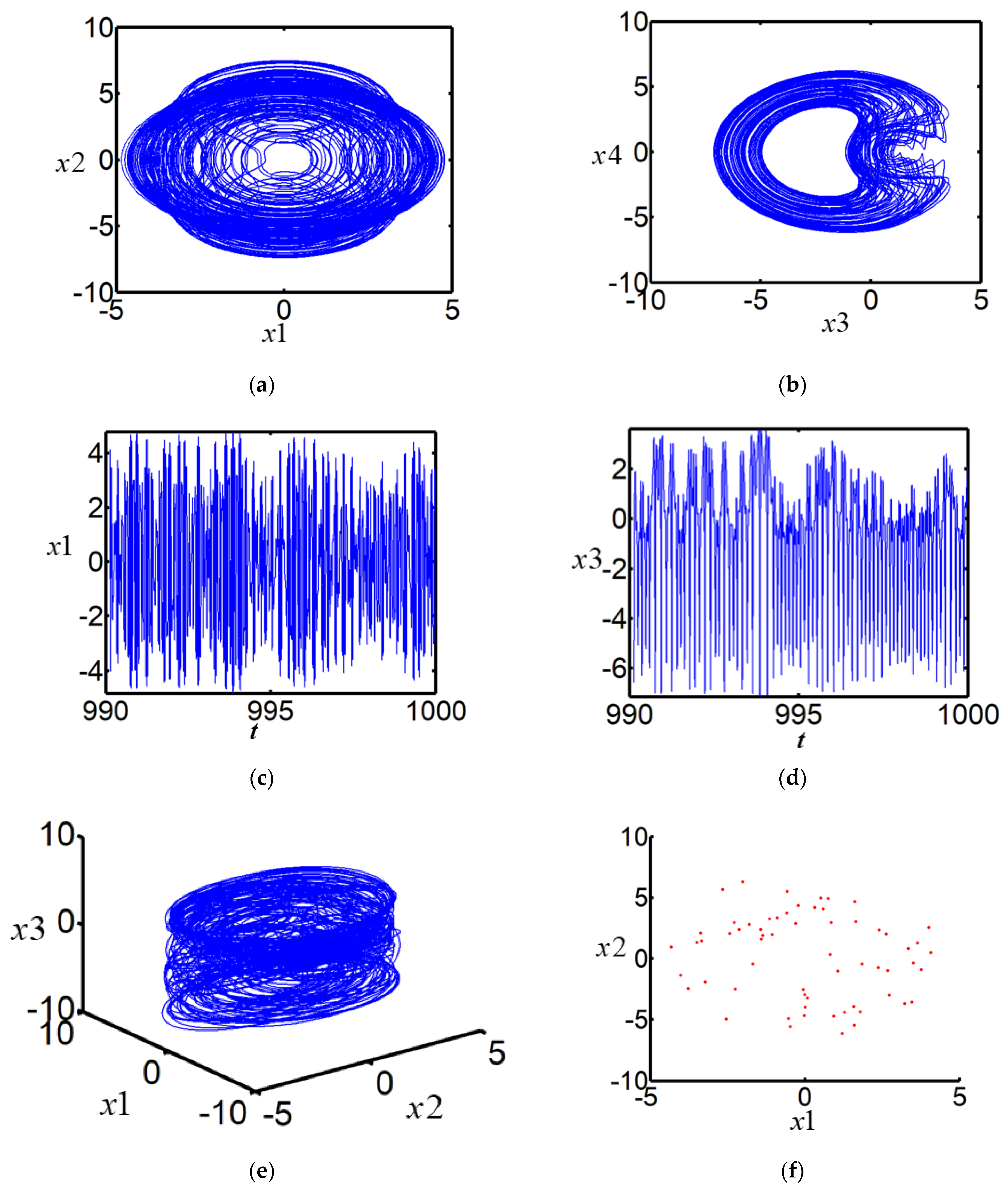
In Figure 3, the parameter f is chosen to be 216.8, with the other parameters maintaining the same as in Figure 1. The nonlinear nonplanar vibration of a cantilever beam is observed in the chaotic motion. Figure 3a–f respectively describe the phase portraits on the planes , , the waveform on the planes , , the phase portraits in the three-dimensional space and the Poincare maps on the plane . By comparing the two-dimensional phase portraits and the three-dimensional phase portraits in Figure 1 and Figure 3, it is found that the cantilever beam will show different chaotic motions when the value of the external excitation is changed. The local activity theory provides a theoretical basis for the parameter selection of the chaotic motion in the cantilever beam. Thus, the motion in chaos can be controlled to a certain extent.
There are several methods to determine whether the system is chaotic or not, such as the phase portraits, the waveform, and Poincare maps. When chaotic motion appears in the system, there are an infinite number of discrete points distributed in the Poincare maps on the plane. When periodic motion appears in the system, there are countable discrete distributed points in the Poincare maps on the plane. Since the Poincare maps on the plane have an infinite number of discrete points distributed, Figure 1, Figure 2 and Figure 3 represent the chaotic motion of the nonlinear nonplanar cantilever beam.
5. Conclusions
In this paper, the local activity theory is used to analyze the nonlinear nonplanar motion of the cantilever beam. Based on the theory of local activity, the local active region of the nonlinear nonplanar motion of a cantilever beam can be calculated. Combined with the actual engineering background and the damping coefficient 0 < c < 1, the cantilever beam is locally active at the equilibrium point only if it satisfies the condition of . Choosing appropriate parameters in the local activity area, the cantilever beam exhibits different types of chaotic motion. The local activity theory provides a mathematically theoretical basis for the analysis and control of the chaotic dynamic behavior of the cantilever beam to a certain extent.
Author Contributions
Conceptualization, M.Z. and Y.X.; methodology, M.Z.; software, P.K. and Y.X.; validation, Y.X.; formal analysis, P.K. and Y.X.; writing—original draft preparation, Y.X.; writing—review and editing, M.Z.; visualization, P.K.; supervision, A.H.; project administration, A.H.; funding acquisition, A.H. All authors have read and agreed to the published version of the manuscript.
Funding
This research is supported by the National Science and Technology Major Project (J2017-II-0009-0023, J2019-V-0017-0112).
Institutional Review Board Statement
Not applicable.
Informed Consent Statement
Not applicable.
Data Availability Statement
Data sharing not applicable.
Conflicts of Interest
The authors declare that there are no conflicting financial interests or personal relationships that could have appeared to influence the work reported in this paper.
Abbreviations
The following abbreviations are used in this manuscript:
| CNN | Convolutional Neural Networks |
| , , , | Real functions |
| Damping coefficient | |
| , | Tuning parameters |
| , , , , | Constants |
| Parametric excitation | |
| , | External excitations |
| Periodic forcing | |
| Jacobian matrix | |
| Equilibrium point | |
| Eigenvalue | |
| Infinitesimal variables | |
| Identity matrix |
References
- Yao, M.H.; Ma, L.; Zhang, W. Study on power generations and dynamic responses of the bistable straight beam and the bistable L-shaped beam. Sci. China-Technol. Sci. 2018, 61, 1404–1416. [Google Scholar] [CrossRef]
- Yao, M.H.; Zhang, W.; Chen, Y.P. Analysis on nonlinear oscillations and resonant responses of a compressor blade. Acta Mech. 2014, 225, 3483–3510. [Google Scholar] [CrossRef]
- Yao, M.H.; Ma, L.; Zhang, W. Nonlinear dynamics of the high-speed rotating plate. Int. J. Aerosp. Eng. 2018, 2018, 5610915. [Google Scholar] [CrossRef] [Green Version]
- Nayfeh, A.H.; Pai, P.F. Non-linear non-planar parametric responses of an inextensional beam. Int. J. Non-Linear Mech. 1989, 24, 139–158. [Google Scholar] [CrossRef]
- Pai, P.F.; Nayfeh, A.H. Non-linear non-planar oscillations of a cantilever beam under lateral base excitations. Int. J. Non-Linear Mech. 1990, 25, 455–474. [Google Scholar] [CrossRef]
- Dwivedy, S.K.; Kar, R.C. Simultaneous combination and 1:3:5 internal resonances in a parametrically excited beam-mass system. Int. J. Non-Linear Mech. 2003, 38, 585–596. [Google Scholar] [CrossRef]
- Young, T.H.; Juan, C.S. Dynamic stability and response of fluttered beams subjected to random follower forces. Int. J. Non-Linear Mech. 2003, 38, 889–901. [Google Scholar] [CrossRef]
- Ma, H.; Zeng, J.; Lang, Z.; Zhang, L.; Guo, Y.; Wen, B. Analysis of the dynamic characteristics of a slant-cracked cantilever beam. Mech. Syst. Signal Process. 2016, 75, 261–279. [Google Scholar] [CrossRef]
- Anderson, T.J.; Nayfeh, A.H.; Balachandran, B. Coupling between high-frequency modes and a low-frequency mode: Theory and experiment. Nonlinear Dyn. 1996, 11, 17–36. [Google Scholar] [CrossRef]
- Cusumano, J.P.; Moon, F.C. Chaotic non-planar vibrations of the thin elastica: Part I: Experimental observation of planar instability. J. Sound Vib. 1995, 179, 185–208. [Google Scholar] [CrossRef]
- Cusumano, J.P.; Moon, F.C. Chaotic non-planar vibrations of the thin elastica: Part II: Derivation and analysis of a low-dimensional model. J. Sound Vib. 1995, 179, 209–226. [Google Scholar] [CrossRef]
- Arafat, H.N.; Nayfeh, A.H.; Chin, C.M. Nonlinear nonplanar dynamics of parametrically excited cantilever beams. Nonlinear Dyn. 1998, 15, 31–61. [Google Scholar] [CrossRef]
- Yao, M.H.; Zhang, W. Multipulse Shilnikov orbits and chaotic dynamics for nonlinear nonplanar motion of a cantilever beam. Int. J. Bifurc. Chaos 2005, 15, 3923–3952. [Google Scholar] [CrossRef]
- Yao, M.H.; Zhang, W. Multi-Pulse chaotic motions of high-dimension nonlinear system for a laminated composite piezoelectric rectangular plate. Meccanica 2014, 49, 365–392. [Google Scholar] [CrossRef]
- Yao, M.H.; Niu, Y.; Hao, Y.X. Nonlinear dynamic responses of rotating pretwisted cylindrical shells. Nonlinear Dyn. 2019, 95, 151–174. [Google Scholar] [CrossRef]
- Yao, M.H.; Chen, Y.P.; Zhang, W. Nonlinear vibrations of blade with varying rotating speed. Nonlinear Dyn. 2012, 68, 487–504. [Google Scholar] [CrossRef]
- Dick, A.J.; Balachandran, B.; Yabuno, H.; Numatsu, M.; Hayashi, K.; Kuroda, M.; Ashida, K. Utilizing nonlinear phenomena to locate grazing in the constrained motion of a cantilever beam. Nonlinear Dyn. 2009, 57, 35–349. [Google Scholar] [CrossRef]
- Yu, Y.P.; Chen, L.H.; Lim, C.W.; Sun, Y.H. Predicting nonlinear dynamic response of internal cantilever beam system on a steadily rotating ring. Appl. Math. Model. 2018, 64, 541–555. [Google Scholar] [CrossRef]
- Francesco, P.P.; Marzia, S.V.B.; Raffaele, B.; Francesco, M.D.S. Random vibrations of stress-driven nonlocal beams with external damping. Meccanica 2020, 56, 1329–1344. [Google Scholar]
- Colgate, J.E.; Schenkel, G.G. Passivity of a class of sampled-data systems: Application to haptic interfaces. J. Robot. Syst. 1997, 14, 37–47. [Google Scholar] [CrossRef]
- Xie, L.; Fu, M.; Li, H. Passivity analysis and passification for uncertain signal processing systems. IEEE Trans. Signal Process. 1998, 46, 2394–2403. [Google Scholar]
- Khan, M.A.; Sahoo, B.; Mondal, A.K. Control of chaos to obtain periodic behaviour via nonlinear control. Proc. Natl. Acad. Sci. India Sect. A-Phys. Sci. 2015, 85, 143–148. [Google Scholar] [CrossRef]
- Pogromsky, A.Y. Passivity based design of synchronizing systems. Int. J. Bifurc. Chaos 1998, 8, 295–319. [Google Scholar] [CrossRef] [Green Version]
- Bemporad, A.; Bianchini, G.; Brogi, F. Passivity analysis and passification of discrete-time hybrid systems. IEEE Trans. Autom. Control 2008, 53, 1004–1009. [Google Scholar] [CrossRef]
- Chua, L.O. Passivity and complexity. IEEE Trans. Circuits Syst. I Fundam. Theory Appl. 1999, 46, 71–82. [Google Scholar] [CrossRef]
- Yang, T.; Chua, L.O. Testing for local activity and edge of chaos. Int. J. Bifurc. Chaos 2001, 11, 1495–1591. [Google Scholar] [CrossRef] [Green Version]
- Chua, L.O. Local activity is the origin of complexity. Int. J. Bifurc. Chaos 2005, 15, 3435–3456. [Google Scholar] [CrossRef] [Green Version]
- Ying, J.J.; Liang, Y.; Wang, J.L.; Dong, Y.J.; Wang, G.Y.; Gu, M.Y. A tristable locally-active memristor and its complex dynamics. Chaos Solitons Fractals 2021, 148, 111038. [Google Scholar] [CrossRef]
- Itoh, M.; Chua, L.O. Oscillations on the edge of chaos via dissipation and diffusion. Int. J. Bifurc. Chaos 2007, 17, 1531–1573. [Google Scholar] [CrossRef]
- Tang, C.; Chen, F.; Wang, J.; Li, X. Extending Local Passivity Theory and Hopf Bifurcation at the Edge of Chaos in Oregonator CNN. Int. J. Bifurc. Chaos 2012, 22, 1250285. [Google Scholar] [CrossRef]
- MatsukI, T.; Shibata, K. Adaptive balancing of exploration and exploitation around the edge of chaos in internal-chaos-based learning. Neural Netw. 2020, 132, 19–29. [Google Scholar] [CrossRef] [PubMed]
- Itoh, M.; Chua, L. Chaotic oscillation via edge of chaos criteria. Int. J. Bifurc. Chaos 2017, 27, 1730035. [Google Scholar] [CrossRef]
- Chua, L.; Sbitnev, V.; Kim, H. Neurons are poised near the edge of chaos. Int. J. Bifurc. Chaos 2012, 22, 1250098. [Google Scholar] [CrossRef]
- Dong, Y.J.; Wang, G.Y.; Chen, G.R.; Shen, Y.R.; Ying, J.J. A bistable nonvolatile locally-active memristor and its complex dynamics. Commun. Nonlinear Sci. Numer. Simul. 2020, 84, 105203. [Google Scholar] [CrossRef]
- Itoh, M. Memristor circuits for simulating nonlinear dynamics and their periodic forcing. Chaotic Dyn. 2019, 19, 07822. [Google Scholar]
Figure 1.
Chaotic motion in nonlinear nonplanar vibration for the cantilever beam: (a) phase portrait on the plane ; (b) phase portrait on the plane ; (c) waveform on the plane ; (d) waveform on the plane ; (e) phase portrait in the three-dimensional space ; (f) Poincare maps on the plane .
Figure 1.
Chaotic motion in nonlinear nonplanar vibration for the cantilever beam: (a) phase portrait on the plane ; (b) phase portrait on the plane ; (c) waveform on the plane ; (d) waveform on the plane ; (e) phase portrait in the three-dimensional space ; (f) Poincare maps on the plane .
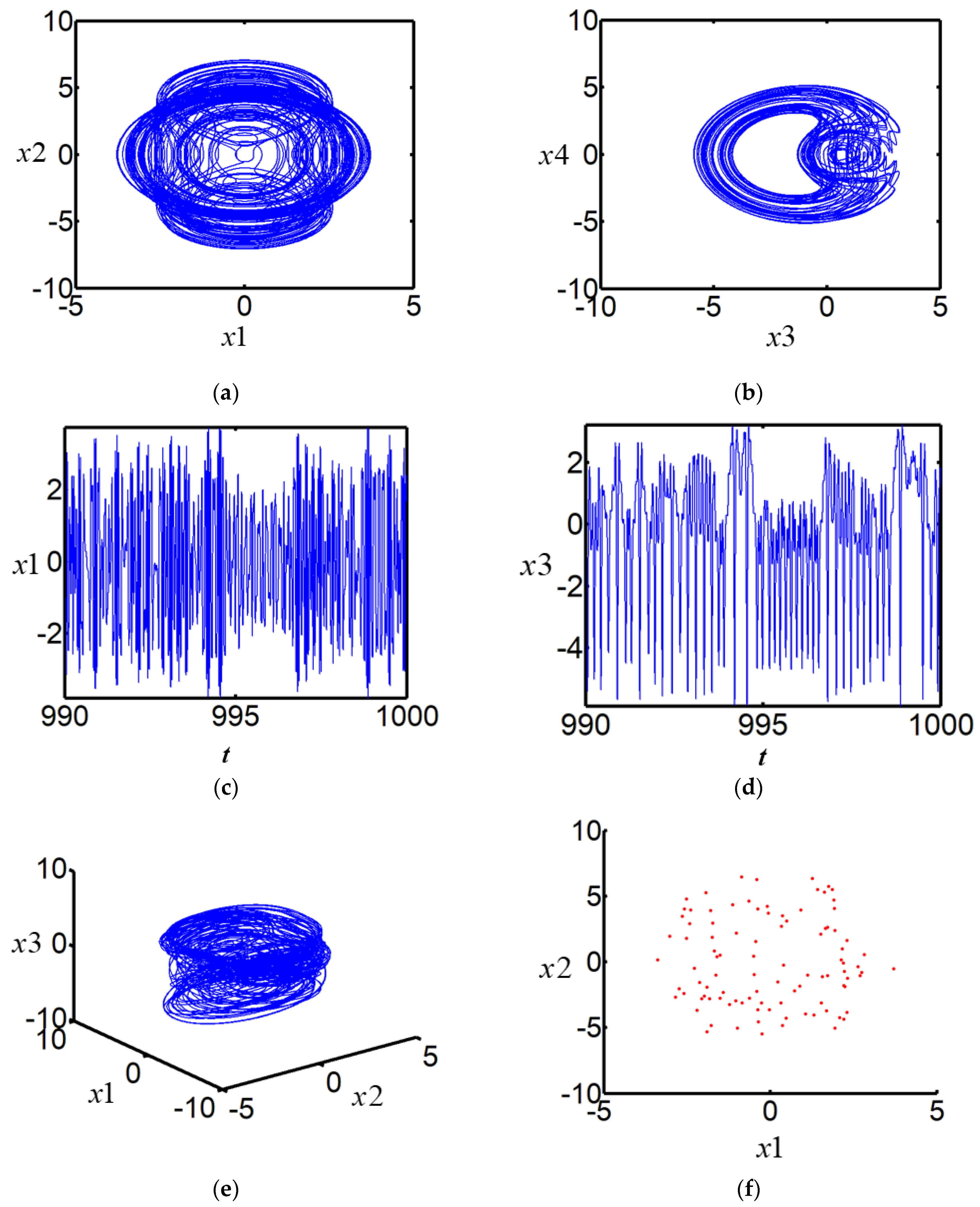
Figure 2.
Chaotic motion in nonlinear vibration for the cantilever beam with parameter change: (a) phase portrait on the plane ; (b) phase portrait on the plane ; (c) waveform on the plane ; (d) waveform on the plane ; (e) phase portrait in the three-dimensional space ; (f) Poincare maps on the plane .
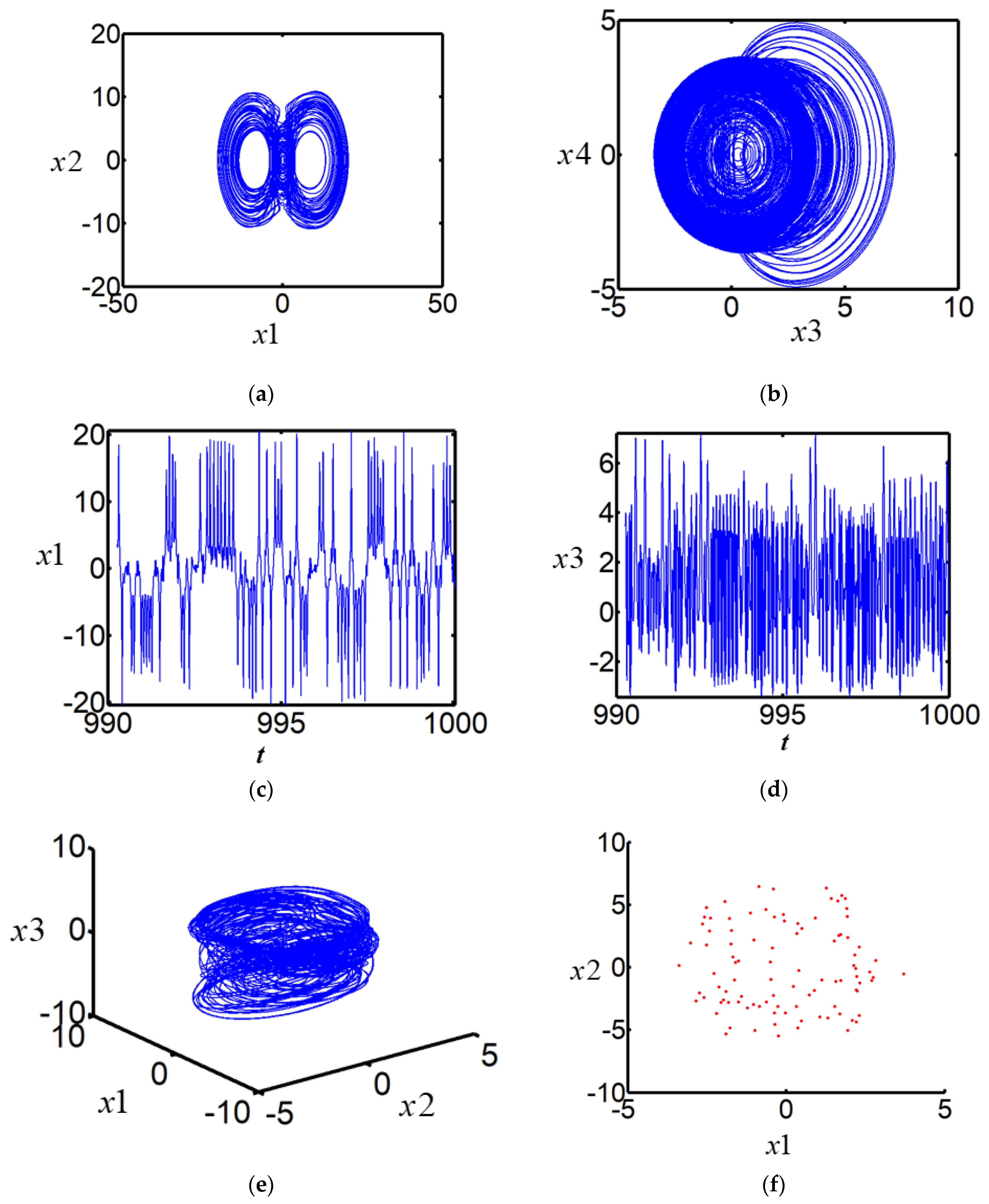
Figure 3.
Nonlinear vibration in chaotic motion for the cantilever beam: (a) phase portrait on the plane ; (b) phase portrait on the plane ; (c) waveform on the plane ; (d) waveform on the plane ; (e) phase portrait in the three-dimensional space ; (f) Poincare maps on the plane .
Figure 3.
Nonlinear vibration in chaotic motion for the cantilever beam: (a) phase portrait on the plane ; (b) phase portrait on the plane ; (c) waveform on the plane ; (d) waveform on the plane ; (e) phase portrait in the three-dimensional space ; (f) Poincare maps on the plane .
Publisher’s Note: MDPI stays neutral with regard to jurisdictional claims in published maps and institutional affiliations. |
© 2022 by the authors. Licensee MDPI, Basel, Switzerland. This article is an open access article distributed under the terms and conditions of the Creative Commons Attribution (CC BY) license (https://creativecommons.org/licenses/by/4.0/).
Share and Cite
MDPI and ACS Style
Zhang, M.; Kong, P.; Hou, A.; Xu, Y. Fractal Analysis of Local Activity and Chaotic Motion in Nonlinear Nonplanar Vibrations for Cantilever Beams. Fractal Fract. 2022, 6, 181. https://doi.org/10.3390/fractalfract6040181
AMA Style
Zhang M, Kong P, Hou A, Xu Y. Fractal Analysis of Local Activity and Chaotic Motion in Nonlinear Nonplanar Vibrations for Cantilever Beams. Fractal and Fractional. 2022; 6(4):181. https://doi.org/10.3390/fractalfract6040181
Chicago/Turabian StyleZhang, Mingming, Pan Kong, Anping Hou, and Yuru Xu. 2022. "Fractal Analysis of Local Activity and Chaotic Motion in Nonlinear Nonplanar Vibrations for Cantilever Beams" Fractal and Fractional 6, no. 4: 181. https://doi.org/10.3390/fractalfract6040181