
A Novel Modeling Method of Micro-Topography for Grinding Surface Based on Ubiquitiform Theory


1
Mechanical Electrical Engineering School, Beijing Information Science & Technology University, Beijing 100192, China
2
Key Laboratory of Modern Measurement and Control Technology, Ministry of Education, Beijing Information Science & Technology University, Beijing 100192, China
3
Department of Mechanical Engineering, State Key Laboratory of Tribology, Tsinghua University, Beijing 100084, China
4
School of Mechanical Electronic & Information Engineering, China University of Mining & Technology-Beijing, Beijing 100083, China
*
Authors to whom correspondence should be addressed.
Fractal Fract. 2022, 6(6), 341; https://doi.org/10.3390/fractalfract6060341
Submission received: 4 May 2022
/
Revised: 13 June 2022
/
Accepted: 16 June 2022
/
Published: 19 June 2022
(This article belongs to the Special Issue Applications of Multifractal Analysis in Surface Science)
Abstract
:In order to simulate the grinding surface more accurately, a novel modeling method is proposed based on the ubiquitiform theory. Combined with the power spectral density (PSD) analysis of the measured surface, the anisotropic characteristics of the grinding surface are verified. Based on the isotropic fractal Weierstrass–Mandbrot (W-M) function, the expression of the anisotropic fractal surface is derived. Then, the lower bound of scale invariance δmin is introduced into the anisotropic fractal, and an anisotropic W-M function with ubiquitiformal properties is constructed. After that, the influence law of the δmin on the roughness parameters is discussed, and the δmin for modeling the grinding surface is determined to be 10−8 m. When δmin = 10−8 m, the maximum relative errors of Sa, Sq, Ssk, and Sku of the four surfaces are 5.98%, 6.06%, 5.77%, and 4.53%, respectively. In addition, the relative errors of roughness parameters under the fractal method and the ubiquitiformal method are compared. The comparison results show that the relative errors of Sa, Sq, Ssk, and Sku under the ubiquitiformal modeling method are 5.36%, 6.06%, 5.84%, and 4.53%, while the maximum relative errors under the fractal modeling method are 23.21%, 7.03%, 83.10%, and 7.25%. The comparison results verified the accuracy of the modeling method in this paper.
1. Introduction
The modeling of machined surfaces has always been a fundamental topic in the field of tribology [1]. An accurate surface can provide a model basis for research on contact characteristics for mechanical joint surfaces, which has practical engineering significance for the design of precision instruments [2]. Grinding is one of the most widely used machining methods and determining how to achieve accurate modeling of the grinding surface has always been a hot topic for relevant scholars [3]. There are three modeling methods of micro-topography for grinding surfaces: The numerical simulation method, geometric simulation method, and fractal modeling method [4,5].
The numerical simulation method simulated the grinding surface by Gaussian or non-Gaussian surfaces [6]. Wu et al. generated Gauss and non-Gauss surfaces separately to simulate grinding surfaces [7,8]. Wang et al. combined Fourier transform with the Johnson conversion system [9] to simulate non-Gaussian surfaces with specific roughness parameters [10]. The advantage of this method is that the simulated surface is based on roughness parameters, which can satisfy the statistical characteristics. However, with deepening research, defects gradually emerged [11,12]. In the simulation process, the truncation length of the autocorrelation function has a great impact on the simulation topography. Improper truncation length of the autocorrelation function may lead to wrong results [12]. Moreover, using Gaussian or non-Gaussian surfaces instead of actual grinding surfaces will introduce errors in the analysis of the contact characteristics [2,13].
The geometric simulation method is based on grinding kinematics theory. Combined with the grinding parameters and the motion trajectory of abrasive particles on a grinding wheel, the simulation of the grinding surface was realized. Based on the grinding parameters, Warneck et al. deduced the motion equation between the grinding wheel and the workpiece [14]. Based on the research of Saini [15], Cooper et al. added the empirical equation of plough and sliding friction in the process of topography simulation [16]. Nguyen et al. developed a numerical simulation program for a grinding surface based on topography data of a grinding wheel and grinding kinematics theory [17,18]. Based on the research of Nguyen, Cao et al. considered the influence of the vibration between the grinding wheel and the workpiece during the simulation of the surface topography [19]. Combined with the Johnson transform [9], Wen conducted simulation research on the theoretical grinding topography based on the topography of the grinding wheel and the grinding kinematics [20]. Chen et al. introduced the waviness information into the simulation process of surface topography [21,22]. Lipiński et al. applied artificial neural networks to the modelling of surface roughness and grinding forces [23].
The advantage of this method is that the simulation method is based on the grinding kinematics theory, which can obtain the influence mechanism of the machining parameters on the grinding topography. However, the following shortcomings cannot be ignored: Firstly, the premise of this method requires an accurate grinding wheel surface, and its modeling accuracy is the basis for ensuring the accuracy of the grinding surface. The abrasive particle distribution or other random variables in the modeling process of grinding wheel surface have always been the key factors affecting the accuracy of grinding wheel surface modeling [24]. Secondly, due to the vibration of the machine, feed error, thermal deformation, and other factors, there is a large deviation between the theoretical topography and the measured topography [25]. In addition, there are many influencing factors in the grinding process, and it is difficult to detect each influencing factor accurately and quantitatively. Therefore, with the deepening of research, the difficulty of analysis will increase greatly [1]. Finally, this method is limited to only realizing the characterization of the grinding surface and cannot provide a model basis for the subsequent analysis of the contact characteristic for the grinding joint surface [26].
The fractal modeling method simulated the grinding surface by fractal surface. Sayles et al. [27] pointed out that the machined surface has fractal characteristics. Majumdar and Bhushan introduced the fractal theory into the field of tribology and used the two-dimensional (2D) W-M function to characterize the rough surface, and then analyzed the contact characteristics of the rough joint surface [28]. Subsequently, Ausloos and Berman extended the 2D W-M function to a three-dimensional (3D) space and derived the generalized expression of 3D W-M function [29]. Later, Yan and Komvopoulos deduced the generalized form of the 3D W-M function and obtained the 3D W-M function in the Cartesian coordinate system [30]. This fractal expression is a common form to characterize rough surfaces [31,32], and many results have been obtained in the analysis of contact characteristics for rough joint surfaces [32,33,34]. However, with the deepening of research, the disadvantages of the fractal modeling method have gradually emerged, especially in the aspect of the fractal measure [5,35,36].
Ou et al. pointed out that the integer dimension measure of a fractal is divergent, and the fractal dimension is discontinuous with respect to the measurement scale [37]. Especially considering the measure, it is unreasonable to describe a physical object with a fractal approximation. Furthermore, after an infinite number of self-similar or self-affine iterative processes, the Hausdorff dimension mutates from an integer dimension to a fractal dimension, which means the integer dimension measure of the fractal has singular characteristics. Therefore, Ou et al. proposed the concept of ubiquitiform on the basis of fractal theory to solve the difficulty caused by the singularity of the fractal measure [37]. The ubiquitiform was defined as a self-similar or self-affine structure with finite levels, which can usually be generated by a finite number of iterations under some given generation rule. Subsequently, the ubiquitiform theory has been applied to the equivalent elastic modulus characterization for a bimaterial bar [38], the one-dimensional steady-state conduction model for a cellular material rod [39], the softening behavior for concrete [40,41], and the research of parameters for material fracture energy characterization [42], the crack propagation in quasi-brittle materials [43], and the mesostructural characterization of polymer-bonded explosives [44]. Relevant scholars have introduced the concept of ubiquitiform theory into the analysis of contact characteristics of rough joint surfaces. Shang et al. studied the normal contact stiffness of rough joint surfaces based on the ubiquitiform theory [45]. Unfortunately, there was no relevant literature on the modeling of grinding surfaces based on ubiquitiform theory.
According to the previous research results of our team, the fractal surface may be more suitable for isotropic machined surfaces such as polishing, electrical discharge machining, or electroplating [1,3,46]. During the analysis of the measured grinding surface [1], it was found that the measured surface has anisotropic characteristics, which are quite different from the commonly used fractal surfaces. Combined with the analysis of grinding kinematics, the grinding surface will show anisotropy in the direction of linear motion of the workpiece. Therefore, the anisotropic ubiquitiform theory is introduced into the modeling of a grinding surface, and the modeling accuracy of the grinding surface is analyzed.
2. Characteristic Analysis of Measured Surfaces
In order to obtain the grinding surface under different ubiquitiformal dimensions, the specimens are prepared by using grinding wheels with different abrasive grains. The 45# steel is selected as the specimen material. The abrasive grains of the grinding wheel are 60#, 80#, 100#, and 120#, respectively. Meanwhile, in order to ensure the reliability of the data, the number of specimens under each abrasive grain is three, and the average values of the three surfaces are taken as the final data for later calculation of the ubiquitiformal dimensions. After the specimens are machined, the micro-topography of grinding surfaces is measured and analyzed. The noncontact micro topography measurement system ZYGONexView (ZYGO Corporation, Middlefield, CT, USA) is used to measure the micro-topography of the grinding surface. The sampling area is 3 mm × 3 mm and the number of sampling points is 1024 × 1024. The sampling method complied with ISO25178-3 [5], and the sampling area conformed to the S-F surface. Figure 1 shows the micro-topography of 45# steel under different roughness.
The arithmetic mean deviations of the surfaces are Sa 0.112 μm, Sa 0.266 μm, Sa 0.403 μm, and Sa 0.672 μm, respectively. Different from the 2D roughness parameter R, the symbol S represents the 3D roughness parameter. For the convenience of distinguishing different surfaces, the rough surfaces are defined as Surface 1, Surface 2, Surface 3, and Surface 4 according to the roughness Sa from small to large. In addition, the coordinate directions involved in the following statements are described with reference to the coordinates in Figure 1.
The power spectral density analysis is performed on the measured grinding surfaces. The calculation flow of 2D power spectral density can be found in Figure S1. Figure 2 shows the 2D power spectral density of the measured surfaces.
It can be seen from Figure 2 that the grinding surface is not an isotropic surface, and exhibits anisotropic characteristics in the y-direction. This result is the same as the result from the literature [47]. Moreover, in the literature, the fractal dimension of the grinding surface at different angles was measured. The results have shown that the fractal dimension of the grinding surface varies greatly under different inclination angles. However, in the y-direction, the error of fractal dimension was small. The results further verify the anisotropic characteristics of the grinding surface.
The following is a supplementary formation analysis of the grinding surface from the perspective of grinding kinematics. During the grinding process, the grinding wheel is in a rotating state, while the workpiece is in a linear motion state. With the relative movement between the grinding wheel and the workpiece, the abrasive particles on the grinding wheel will leave a trajectory on the surface of the workpiece. If a certain circumferential section of the grinding wheel is selected as the reference coordinate system, the workpiece surface will move relative to the section of the grinding wheel, and this grinding wheel section will leave a trajectory in the direction of workpiece movement. Moreover, this continuous trajectory also has anisotropic characteristics. This viewpoint is consistent with the geometric simulation method.
In conclusion, based on the power spectral density analysis and grinding kinematics analysis of the measured grinding surface, the anisotropic characteristics of the surface topography are verified. In the next section, the modeling method will be described in detail.
3. Modeling Method
Different from the regular tool shapes such as turning and milling, there are essential differences in the formation of the grinding surface. Due to the disordered and irregular shape of abrasive particles on the grinding wheel’s surface, the modeling of the grinding surface has always been a difficult problem. In the case of not analyzing the measured grinding surface, relevant scholars proposed the use of a fractal surface to simulate the grinding surface [22,48]. The current fractal modeling methods and defects are described in this section. Then, the lower bound of scale invariance δmin is introduced into the anisotropic fractal, and an anisotropic W-M function with ubiquitiformal properties is constructed, which provides a theoretical basis for the construction of a ubiquitiformal surface.
3.1. Modeling Method Based on Fractal Theory
Majumdar and Bhushan introduced fractal theory into the field of tribology and used the 2D W-M function to characterize the rough surface [28]. With the increase in research, Ausloos and Berman extended the 2D W-M function to 3D space and derived the generalized expression of the 3D W-M function. The expression is shown in Equation (1) [29].
where W(r) is the vertical height of the 3D fractal surface; D is the fractal dimension of the fractal surface, and 2 < D < 3; G is the scale coefficient of the fractal surface; γ is the frequency density parameter of the fractal surface, and the rough surface that satisfies the normal distribution takes γ = 1.5, where γn refers to the spatial frequency on the surface. Exp is an exponential function; k0 is the wave number on the surface, which satisfies the relation k0 = 2π/L, the sampling length L; M is the number of overlapping wrinkles on the fractal surface. When M = 1, the surface is anisotropic, and when M ≠ 1, the surface is isotropic. Am is the height of the highest point on the fractal surface, and it satisfies the relation Am = 2π(2π/G)2-D; αm is used to represent the direction of the wave corresponding to m on the rough surface, which satisfies the relation αm = πm/M; φm,n is the random phase, where the value range is [0, 2π]. N is the frequency index of the asperity, and its value range is (-∞, +∞).
Yan and Komvopoulos deduced the generalized form of the 3D W-M function, and obtained the 3D W-M function in the Cartesian coordinate system. The functional expression is shown in Equation (2) [30].
Different from Equation (1), z is the vertical height of the fractal surface, x and y are the coordinates of the data points in the x and y directions, respectively, and the value range of n is (nl, nmax).
The frequency index n of the asperity is introduced in detail below. According to Equation (2), the value range of n is (nl, nmax), where nl is the lower limit of the frequency index, and nmax is the upper limit of the frequency index. For a fractal surface, the calculation formula of nl is shown in Equation (3).
where L is the sample length and floor is the rounding function. Since n cannot be made to tend to infinity during the surface simulation, it is necessary to restrict the high-frequency part of the function, that is, the frequency exponent nl = 0.
According to reference [30], the equation of the upper limit of the frequency index nmax is as follows.
where Ls is the resolution of the measuring instrument.
Based on the analysis of the measured surface in Section 2, the grinding surface has anisotropic characteristics. This result obviously contradicts the isotropic characteristics of the fractal surface. Therefore, based on the existing isotropic fractal W-M function, the anisotropic fractal function is derived. It can be seen from the literature [30] that when the number of overlapping wrinkles M = 1, the fractal surface will appear anisotropic. Therefore, by inserting M = 1 into Equation (2) and simplifying it, the form shown in Equation (5) can be obtained. Equation (5) shows the equation of the anisotropic fractal surface.
Based on the above analysis, the equations of isotropic and anisotropic fractal surfaces can be obtained, as shown in Equation (2) and Equation (5), respectively. The numerical simulation of the above two surfaces is carried out using Matlab software (R2018b, MathWorks, Natick, MA, USA). The simulation process can be divided into the following four steps: Firstly, the initial values for simulation need to be inputted. The initial values are γ = 1.5, L = 3 × 10⁻³ m, Ls = 5 × 10⁻⁸ m, D = 2.4, G = 10−13, and φm,n = π/6. In addition, the values of M are 10 and 1, respectively. Secondly, the simulation area is set and interpolated. A 256 × 256 interpolation is performed on the simulation area in this paper, and the data after interpolation are taken as the x and y coordinate values. The next step is to use m and n as loop variables to calculate the vertical height z of the fractal surface. Through the above process, the topography of the 3D fractal surface can be obtained. Finally, the vertical height under the corresponding coordinates is displayed graphically.
It should be noted that fractal dimension D and scale coefficient G are the characteristic parameters of the fractal surface. Figure 3 shows the isotropic fractal surface and the anisotropic fractal surface under D = 2.4 and G = 1 × 10⁻¹³, respectively.
Combined with Figure 1 and Figure 3 for analysis, compared with the isotropic fractal surface, the anisotropic fractal surface has a higher similarity to the measured surface. It is worth noting that since the fractal characteristic parameters are randomly selected, the fractal surface may differ in detail from the measured surface. In other words, the above surface is only a qualitative reference.
3.2. Modeling Method Based on Ubiquitiform Theory
Based on the analysis in Section 3.1, the equation of the anisotropic fractal surface can be obtained. However, in combination with Equation (4), when the resolution of the measuring instrument Ls changes, the fractal characteristic parameters of the same rough surface will change accordingly, and then there will be differences in the simulated surfaces.
Compared with fractal theory, the description of actual physical objects in ubiquitiform theory does not have arbitrarily small details and infinite iterations. Therefore, the ubiquitiform theory is introduced into the modeling of the grinding surface, and the concept of minimum infimum is introduced into the modeling process of the rough surface. The minimum infimum of the rough surface is closely related to the surface topography. It is generally believed that the minimum infimum is the same as the lower bound of scale invariance of the rough surface, that is, the minimum infimum is the lower bound of scale invariance δmin. For a given rough surface, the δmin is a fixed value, which will not change with the resolution of the measuring instrument.
Based on the above analysis, combined with δmin and Equation (4), the upper limit of the frequency index nmax is redefined, as shown in Equation (6).
Combining Equations (5) and (6), the equation of the anisotropic surface with ubiquitiformal properties can be constructed, as shown in Equation (7).
Under the ubiquitiform theory, due to the existence of the lower bound to scale invariance δmin, the ubiquitiform has an integer Hausdorff dimension, which is equal to the corresponding topological dimension. The research on practical problems under ubiquitiform theory can avoid many problems caused by the singularity of the integer dimension measure and measure singularity in the fractal theory.
The lower bound of scale invariance δmin is introduced into the anisotropic fractal in this section, and the equation of anisotropic surface with ubiquitiformal properties is constructed. It should be noted that, corresponding to the fractal surface, the fractal dimension D, the scale coefficient G, and the lower bound of scale invariance δmin are the characteristic parameters of the ubiquitiformal surface. In order to explore the influence of the lower bound to scale invariance δmin on the simulation surface, different δmin values are taken for analysis. The δmin is taken as 10−3 m, 10−5 m, 10−7 m, and 10−9 m, respectively. Other initial values for simulation are taken as M = 1; γ = 1.5; L = 3 × 10⁻³ m; D = 2.4; G = 10−13; φm,n = π/6. The simulation flow is described in Section 3.1. The modeling results of ubiquitiformal surfaces under different δmin values are shown in Figure 4.
It can be seen from Figure 4 that with the decrease in δmin, the details of the ubiquitiformal surface increase gradually. When δmin = 10−3 m, there is a clear difference between the surfaces under other δmin conditions. However, with the decrease in the δmin, the change in surface details is not obvious. Therefore, in combination with roughness parameters, the quantitative analysis of the modeling error of the ubiquitiformal surface will be presented in the next section.
4. Modeling of Grinding Surface
In order to verify the accuracy of the modeling method in this paper, the fractal surface and the ubiquitiformal surface are compared and analyzed in this section. The box-counting method [49] is used to obtain the fractal characteristic parameters of the measured grinding surface. The fractal characteristic parameters of different grinding surfaces are shown in Table 1.
The above fractal characteristic parameters are used for the modeling of fractal surfaces and ubiquitiformal surfaces, respectively. The simulation process is described in Section 3.1. The initial values for simulation are taken as γ = 1.5; L = 3 × 10⁻³ m; Ls = 1 × 10⁻⁸ m; φm,n = π/6. The values of M are 10 and 1, respectively. The fractal characteristic parameters are taken according to Table 1. In addition, the value of the ubiquitiformal feature parameter δmin is 10−8 m. The simulated fractal surfaces and ubiquitiformal surfaces based on the fractal characteristic parameters of measured surfaces are shown in Figure 5 and Figure 6, respectively.
Based on the fractal characteristic parameters of measured surfaces, the fractal surfaces and the ubiquitiformal surfaces are constructed in this section. Compared with the measured surfaces in Figure 1, it can be seen that the ubiquitiformal surfaces have a higher similarity than the fractal surfaces. Subsequently, the relative errors of roughness parameters will be compared and analyzed in the next section.
5. Results Comparison
Combined with the analysis in Section 4, based on the fractal characteristic parameters of measured surfaces, the fractal surfaces and the ubiquitiformal surfaces are constructed. Combined with specific roughness parameters, the relative errors of the ubiquitiformal surface under different δmin values are compared, and then the relative errors under two modeling methods are analyzed. Four parameters including the arithmetic mean deviation Sa, root mean square deviation Sq, skewness Ssk, and kurtosis Sku are selected as measurement standards to calculate and analyze the relative error.
5.1. Different Lower Bound to Scale Invariance δmin
In order to explore the influence of the lower bound of scale invariance δmin on the roughness parameters, the relative errors of roughness parameters under different δmin values are compared and analyzed. The δmin is taken as 1 × 10⁻³ m, 1 × 10⁻⁴ m, 1 × 10⁻⁵ m, 1 × 10⁻⁶ m, 1 × 10⁻⁷ m, 1 × 10⁻⁸ m, 1 × 10⁻⁹ m, and 1 × 10⁻¹⁰ m. The other initial values for simulation are as follows: M = 1; γ = 1.5; L = 3 × 10⁻³ m; φm,n = π/6. Meanwhile, the values of other ubiquitiformal characteristic parameters are selected according to Table 1. The relative errors of roughness parameters under different δmin are shown in Figure 7. Moreover, the relative error value can be found in Tables S1–S4 in the Supplementary Materials.
From the overall presentation of Figure 7, the relative error of each roughness parameter decreases with the decrease in the δmin. When δmin = 10−8 m, the relative error of each roughness parameter tends to be stable. The following is the separate analysis for the four roughness parameters.
Figure 7a shows the relative errors of the roughness parameter Sa. With the decrease in δmin, the relative error of the surface roughness Sa shows a decreasing trend. In the range of 10−3 m > δmin > 10−8 m, the relative error decline rate of Sa gradually decreases. When δmin < 10−8 m, the relative error of Sa tends to be stable. When δmin = 10−8 m, the relative errors of the four surfaces are 5.98%, 2.22%, 0.40%, and 0.67%, respectively. It can be seen that when δmin = 10−8 m, the maximum relative error of Sa is 5.98%. For surface 1, there is a sharp drop in the relative error of Sa at δmin = 10−5 m. The reason may be that the size of abrasive particles on the grinding wheel is small and the surface topography of the grinding wheel is disordered, resulting in a large deviation between the simulated surface and the measured surface. In the range of 10−5 m > δmin > 10−8 m, the relative error of Sa shows a gradual upward trend, which also confirms the above point of view. With a further decrease in δmin, the relative error of Sa also tends to be stable.
In addition, under the conditions of the same δmin, the relative error of Sa decreases gradually with the increase in surface roughness. With the increase in surface roughness, the size of abrasive particles on the grinding wheel increases gradually. Combined with the analysis of the measured grinding surface characteristics in Section 2, the measured surface topography is more in line with the ubiquitiformal surface, resulting in the relative error of Sa gradually decreasing with the increase in surface roughness.
Figure 7b shows the relative error of the roughness parameter Sq. With the decrease in δmin, the relative error of the surface roughness Sq has a decreasing trend. In the range of 10−3 m > δmin > 10−8 m, the relative error decline rate of Sq gradually decreases. When δmin < 10−8 m, the relative error of Sq tends to be stable. When δmin = 10−8 m, the relative errors of Sq of the four surfaces are 6.06%, 5.35%, 3.70%, and 3.44%, respectively. It can be seen that when δmin = 10−8 m, the maximum relative error of Sq is 6.06%. Different from the variation trend of the relative error of the roughness parameter Sa, with the decrease in δmin, the relative error of Sq maintained a downward trend. In addition, under the same δmin, the relative error of Sq decreases gradually with the increase in surface roughness. With the increase in surface roughness, the size of abrasive particles on the grinding wheel increases gradually. Combined with the analysis of the measured grinding surface characteristics in Section 2, the measured surface topography is more in line with the ubiquitiformal surface, resulting in the relative error of Sq decreasing gradually with the increase in surface roughness.
Figure 7c shows the relative error of the roughness parameter Ssk. With the decrease in δmin, the relative error of the surface roughness Ssk shows a decreasing trend. In the range of 10−3 m > δmin > 10−5 m, the relative error decline rate of Ssk decreases gradually. When 10−5 m > δmin > 10−8 m, the relative error of Ssk fluctuates up and down. When δmin < 10−8 m, the relative error of Ssk tends to be stable. When δmin = 10−8 m, the relative errors of Ssk on the four surfaces are 4.23%, 2.33%, 5.77%, and 5.11%, respectively. It can be seen that when δmin = 10−8 m, the maximum relative error of Ssk is 5.77%. Ssk is the skewness characteristic of the height distribution of the rough surface. Due to the disorder of the grinding wheel surface, the deflection of the rough surface is not a controllable factor. However, it is worth noting that the relative error of the roughness parameter Ssk obtained by the ubiquitiformal modeling method has a small error regarding the measured surface.
Figure 7d shows the relative error of the roughness parameter Sku. With the decrease in δmin, the relative error of the surface roughness Sku has a decreasing trend. In the range of 10−3 m > δmin > 10−5 m, the relative error decline rate of Sku decreases gradually. When 10−5 m > δmin > 10−8 m, the relative error of Sku fluctuates up and down. When δmin < 10−8 m, the relative error of Ssk tends to be stable. When δmin = 10−8 m, the relative errors of Sku on the four surfaces are 4.36%, 4.53%, 3.73%, and 4.12%, respectively. It can be seen that when δmin = 10−8 m, the maximum relative error of Ssk is 4.53%. Ssk is the kurtosis characteristic of the height distribution of the rough surface. Due to the disorder of the grinding wheel surface, the deflection of the rough surface is not a controllable factor. However, it is worth noting that the ubiquitiformal modeling method has a small error regarding the measured surface.
Based on the above analysis, the relative error of each roughness parameter decreases gradually with the decrease in δmin. When δmin = 10−8 m, the relative error of each roughness tends to be stable. Combined with the analysis of the resolution for the surface-measuring instrument, improving the resolution of the measuring instrument will undoubtedly increase the cost of surface topography measurement. Therefore, combined with the rough surface modeling accuracy and measurement cost, the δmin value for modeling the grinding surface is determined to be 10−8 m. When δmin = 10−8 m, the maximum relative errors of Sa, Sq, Ssk, and Sku of the four surfaces are 5.98%, 6.06%, 5.77%, and 4.53%, respectively.
5.2. Different Modeling Methods
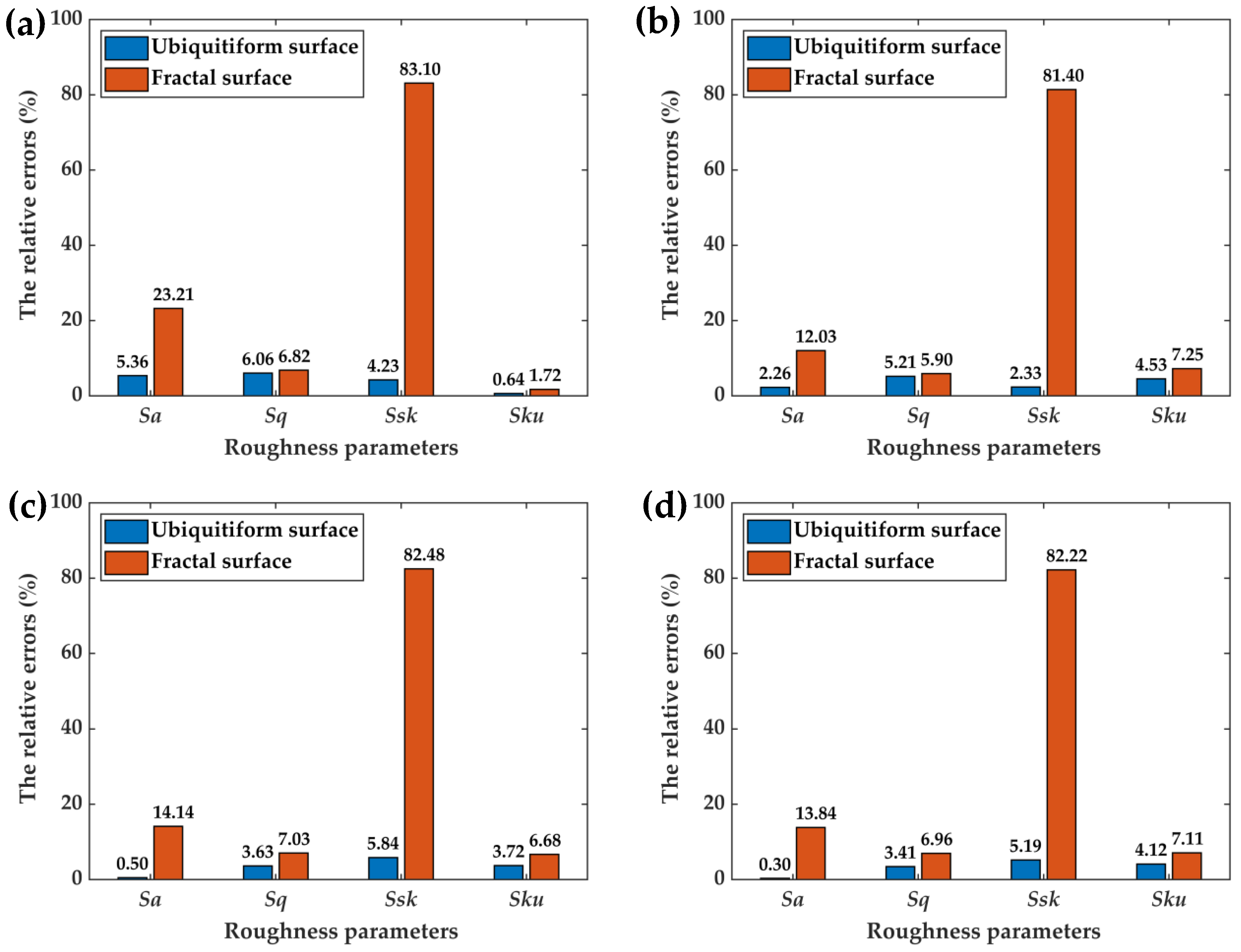
In order to verify the accuracy of the method in this paper, the relative errors of roughness under different modeling methods are compared and analyzed. The compared modeling methods are the fractal modeling method and the ubiquitiformal modeling method. The following is a comparison and analysis of the relative errors of roughness parameters under different modeling methods. The initial values for simulation are as follows: γ = 1.5; L = 3 × 10⁻³ m; Ls = 1 × 10⁻⁶ m; φm,n = π/6; δmin = 10−8 m. Meanwhile, the values of other characteristic parameters are selected according to Table 1. The relative errors of roughness parameters under different modeling methods are shown in Figure 8. Moreover, the relative error value can be found in Tables S5–S8 in the supplementary information.
From the overall presentation of Figure 8, the relative error of each roughness parameter of the ubiquitiformal surfaces is smaller than those of the fractal surfaces, especially the roughness parameter Ssk. The following is the separate analysis for the four roughness parameters.
The first is the relative error of the roughness parameter Sa. The relative errors of Sa under the ubiquitiformal surfaces are 5.36%, 2.26%, 0.50%, and 0.30%, respectively. The relative error of Sa decreases gradually with the increase in surface roughness. With the increase in surface roughness, the size of the abrasive particles on the grinding wheel increases gradually. Combined with the analysis of the measured grinding surface characteristics in Section 2, the measured surface topography is more in line with the ubiquitiformal surface, resulting in the relative error of Sa gradually decreasing with the increase in surface roughness. In obvious contrast with the ubiquitiformal surfaces, the relative errors of Sa under the fractal surfaces are 23.21%, 12.03%, 0.50%, and 0.30%, respectively. Overall, the relative errors of Sa under the fractal modeling method and ubiquitiformal modeling method are quite different. More importantly, the simulated surfaces based on the ubiquitiform theory are closer to the measured surfaces.
The second is the relative error of the roughness parameter Sq. The relative errors of Sa under the ubiquitiformal surfaces are 6.06%, 5.21%, 3.63%, and 3.41%, respectively. Similar to the variation trend of the relative error of Sa, the relative error of Sq decreases gradually with the increase in surface roughness. The reason for this phenomenon is the same as the parameter Sa. Correspondingly, the relative errors of Sq under the fractal surfaces are 6.82%, 5.90%, 7.03%, and 6.96%, respectively. Overall, the relative errors of Sq under two modeling methods are small.
The third is the relative error of the roughness parameter Ssk. This parameter is also the one with the largest difference. The relative errors of Ssk under the ubiquitiformal surfaces are 4.23%, 2.33%, 5.84%, and 5.19%, respectively. For different rough surfaces, the relative error of Ssk has no obvious change rule. In obvious contrast with the ubiquitiformal surface, the relative errors of Ssk under the fractal surfaces are 83.10%, 81.40%, 82.48%, and 82.22%, respectively. The relative error of this parameter is undoubtedly huge. The relative error of this parameter is undoubtedly huge. The Ssk is the skewness characteristic of the height distribution of the rough surface. Due to the self-similarity of the fractal surface, the relative errors of Ssk on the fractal surface are far from the measured surfaces.
The last is the relative error of the roughness parameter Sku. The relative errors of Sku under the ubiquitiformal surfaces are 0.64%, 4.53%, 3.72%, and 4.12%, respectively. For different rough surfaces, the relative error of Sku has no obvious change rule. Correspondingly, the relative errors of Sku under the fractal surfaces are 1.72%, 7.25%, 6.68%, and 7.11%, respectively. Overall, the relative errors of Sku under two modeling methods are small.
Based on the analysis of the above results, the relative error of the roughness parameters under the ubiquitiformal modeling method is smaller than those of the fractal modeling method, especially the roughness parameter Ssk. The comparison results show that the maximum relative errors of Sa, Sq, Ssk, and Sku under the ubiquitiformal modeling method are 5.36%, 6.06%, 5.84%, and 4.53%, respectively. In contrast, the maximum relative errors under the fractal modeling method are 23.21%, 7.03%, 83.10%, and 7.25%, respectively. The comparison results verify the accuracy of the method in this paper.
6. Conclusions
The modeling method of the surface micro-topography under the grinding machining model is studied in this paper. Based on the ubiquitiform theory, a novel modeling method is proposed. The implementation process of this novel method is introduced in detail in this paper. The comparison results show that δmin directly affects the modeling accuracy. Combined with the rough surface modeling accuracy and measurement cost, δmin for modeling the grinding surface is determined to be 10−8 m. Compared with the existing fractal modeling methods, the presented method is more accurate. The research in this paper provides a novel modeling method for the grinding surface, and also provides a model basis for the subsequent analysis of the contact characteristic for the grinding joint surface.
However, the presented method in this paper has higher accuracy for modeling the grinding surface. Whether this method can be applied to surface modeling under other machining modes remains to be further studied. The broad applicability of this method will be explored in future work.
Supplementary Materials
The following supplementary information can be downloaded at: https://www.mdpi.com/article/10.3390/fractalfract6060341/s1, Figure S1: The calculation flow chart of 2D power spectral density; Table S1: The relative errors of roughness parameters under different δmin—Surface 1; Table S2: The relative errors of roughness parameters under different δmin—Surface 2; Table S3: The relative errors of roughness parameters under different δmin—Surface 3; Table S4: The relative errors of roughness parameters under different δmin—Surface 4; Table S5: The relative errors of roughness parameters under different modeling methods—Surface 1; Table S6: The relative errors of roughness parameters under different modeling methods—Surface 2; Table S7: The relative errors of roughness parameters under different modeling methods—Surface 3; Table S8: The relative errors of roughness parameters under different modeling methods—Surface 4.
Author Contributions
Conceptualization and methodology, Y.L. and Q.A.; validation, Q.A., D.S., L.B. and M.H.; writing—original draft preparation and visualization, Y.L., Q.A. and M.H. All authors have read and agreed to the published version of the manuscript.
Funding
This work is financially supported by the National Natural Science Foundation of China (No. 52174154) and the National Natural Science Foundation of China (No. 11802035).
Data Availability Statement
Data are contained within the article or supplementary material. The data presented in this study are available in supplementary materials.
Conflicts of Interest
The authors declare no conflict of interest.
References
- An, Q.; Suo, S.; Bai, Y. A novel simulation method of micro-topography for grinding surface. Materials 2021, 14, 5128. [Google Scholar] [CrossRef]
- An, Q.; Suo, S.; Lin, F.; Shi, J. A novel micro-contact stiffness model for the grinding surfaces of steel materials based on cosine curve-shaped asperities. Materials 2019, 12, 3561. [Google Scholar] [CrossRef] [Green Version]
- Liu, Y.; An, Q.; Shang, D.; Bai, L.; Huang, M.; Huang, S. Research on normal contact stiffness of rough joint surfaces machined by turning and grinding. Metals 2022, 12, 669. [Google Scholar] [CrossRef]
- Anand, R.S.; Patra, K. Modeling and simulation of mechanical micro-machining—A review. Mach. Sci. Technol. 2014, 18, 323–347. [Google Scholar] [CrossRef]
- Magsipoc, E.; Zhao, Q.; Grasselli, G. 2D and 3D roughness characterization. Rock Mech. Rock Eng. 2020, 53, 1495–1519. [Google Scholar] [CrossRef]
- Minet, C.; Brunetiere, N.; Tournerie, B.; Fribourg, D. Analysis and modeling of the topography of mechanical seal faces. Tribol. Trans. 2010, 53, 799–815. [Google Scholar] [CrossRef]
- Wu, J.J. Simulation of rough surfaces with FFT. Tribol. Int. 2000, 33, 47–58. [Google Scholar] [CrossRef]
- Wu, J.J. Simulation of non-Gaussian surfaces with FFT. Tribol. Int. 2004, 37, 339–346. [Google Scholar] [CrossRef]
- Johnson, N.L. Systems of frequency curves generated by methods of translation. Biome 1949, 36, 149–176. [Google Scholar] [CrossRef]
- Wang, Y.; Ying, L.; Zhang, G.; Wang, Y. A simulation method for non-Gaussian rough surfaces using FFT and translation process theory. J. Tribol. 2017, 140, 021403. [Google Scholar] [CrossRef]
- Patrikar, R.M. Modeling and simulation of surface roughness. Appl. Surf. Sci. 2004, 228, 213–220. [Google Scholar] [CrossRef]
- Pawlus, P.; Michalczewski, R.; Lenart, A.; Dzierwa, A. The effect of random surface topography height on fretting in dry gross slip conditions. ARCHIVE Proc. Inst. Mech. Eng. Part J J. Eng. Tribol. 2014, 228, 1374–1391. [Google Scholar] [CrossRef]
- Zhao, G.; Xiong, Z.; Xin, J.; Hou, L.; Gao, W. Prediction of contact stiffness in bolted interface with natural frequency experiment and FE analysis. Tribol. Int. 2018, 127, 157–164. [Google Scholar] [CrossRef]
- Warnecke, G.; Zitt, U. Kinematic simulation for analyzing and predicting high-performance grinding processes. CIRP Annals-Manuf. Technol. 1998, 47, 265–270. [Google Scholar] [CrossRef]
- Saini, D.P. Wheel hardness and local elastic deflections in grinding. Int. J. Mach. Tools Manuf. 1990, 30, 637–649. [Google Scholar] [CrossRef]
- Cooper, W.L.; Lavine, A.S. Grinding process size effect and kinematics numerical analysis. J. Manuf. Sci. Eng. 2000, 122, 59–69. [Google Scholar] [CrossRef]
- Nguyen, T.A.; Butler, D.L. Simulation of precision grinding process, part 1: Generation of the grinding wheel surface. Int. J. Mach. Tools Manuf. 2005, 45, 1321–1328. [Google Scholar] [CrossRef]
- Nguyen, T.A.; Butler, D.L. Simulation of surface grinding process, part 2: Interaction of the abrasive grain with the workpiece. Int. J. Mach. Tools Manuf. 2005, 45, 1329–1336. [Google Scholar] [CrossRef]
- Cao, Y.; Guan, J.; Li, B.; Chen, X.; Yang, J.; Gan, C. Modeling and simulation of grinding surface topography considering wheel vibration. Int. J. Adv. Manuf. Technol. 2013, 66, 937–945. [Google Scholar] [CrossRef]
- Wen, X.N. Modeling and predicting surface roughness for the grinding process. Appl. Mech. Mater. 2014, 599–601, 622–625. [Google Scholar] [CrossRef]
- Chen, S.; Chi, F.C.; Zhang, F.; Zhao, C. Three-dimensional modelling and simulation of vibration marks on surface generation in ultra-precision grinding. Precis. Eng. 2018, 53, 221–235. [Google Scholar] [CrossRef]
- Chen, C.; Tang, J.; Chen, H.; Zhu, C. Research about modeling of grinding workpiece surface topography based on real topography of grinding wheel. Int. J. Adv. Manuf. Technol. 2017, 93, 2411–2421. [Google Scholar] [CrossRef]
- Lipiński, D.; Bałasz, B.; Rypina, Ł. Modelling of surface roughness and grinding forces using artificial neural networks with assessment of the ability to data generalisation. Int. J. Adv. Manuf. Technol. 2018, 94, 1335–1347. [Google Scholar] [CrossRef] [Green Version]
- Zhu, W.-L.; Beaucamp, A. Compliant grinding and polishing: A review. Int. J. Mach. Tools Manuf. 2020, 158, 103634. [Google Scholar] [CrossRef]
- Chi, J.; Guo, J.L.; Chen, L.Q. The study on a simulation model of workpiece surface topography in external cylindrical grinding. Int. J. Adv. Manuf. Technol. 2016, 82, 939–950. [Google Scholar] [CrossRef]
- Yp, A.; Ping, Z.A.; Ying, Y.A.; Aa, B.; Yw, A.; Dg, A.; Sgcde, F. New insights into the methods for predicting ground surface roughness in the age of digitalisation. Precis. Eng. 2021, 67, 393–418. [Google Scholar] [CrossRef]
- Sayles, R.S.; Thomas, T.R. Surface topography as a nonstationary random process. Nature 1978, 271, 431–434. [Google Scholar] [CrossRef]
- Majumdar, A.; Bhushan, B. Fractal model of elastic-plastic contact between rough surfaces. J. Tribol.-Trans. ASME 1991, 113, 1–11. [Google Scholar] [CrossRef]
- Ausloos, M.; Berman, D.H. A multivariate Weierstrass–Mandelbrot function. Proc. R. Soc. Lond. A Math. Phys. Sci. 1997, 400, 331–350. [Google Scholar] [CrossRef]
- Yan, W.; Komvopoulos, K. Contact analysis of elastic-plastic fractal surfaces. J. Appl. Phys. 1998, 84, 3617–3624. [Google Scholar] [CrossRef]
- Shi, W.B.; Zhang, Z.S. Contact characteristic parameters modeling for the assembled structure with bolted joints. Tribol. Int. 2022, 165, 107272. [Google Scholar] [CrossRef]
- Zhao, Y.S.; Wu, H.C.; Liu, Z.F.; Cheng, Q.; Yang, C.B. A novel nonlinear contact stiffness model of concrete-steel joint based on the fractal contact theory. Nonlinear Dyn. 2018, 94, 151–164. [Google Scholar] [CrossRef]
- Zheng, J.L.; Liu, X.K.; Jin, Y.; Dong, J.B.; Wang, Q.Q. Effects of surface geometry on advection-diffusion process in rough fractures. Chem. Eng. J. 2021, 414, 128745. [Google Scholar] [CrossRef]
- Liu, Y.; Wang, Y.S.; Chen, X.; Yu, H.C. A spherical conformal contact model considering frictional and microscopic factors based on fractal theory. Chaos Solitons Fractals 2018, 111, 96–107. [Google Scholar] [CrossRef]
- Jiang, K.; Liu, Z.F.; Yang, C.B.; Zhang, C.X.; Tian, Y.; Zhang, T. Effects of the joint surface considering asperity interaction on the bolted joint performance in the bolt tightening process. Tribol. Int. 2022, 167, 107408. [Google Scholar] [CrossRef]
- Li, L.; Yun, Q.Q.; Li, Z.Q.; Liu, Y.; Cao, C.Y. A new contact model of joint surfaces accounting for surface waviness and substrate deformation. Int. J. Appl. Mech. 2019, 11, 1950079. [Google Scholar] [CrossRef]
- Ou, Z.C.; Li, G.Y.; Duan, Z.P.; Huang, F.L. Ubiquitiform in applied mechanics. J. Theor. Appl. Mech. 2014, 52, 37–46. [Google Scholar]
- Yang, M.; Ou, Z.C.; Duan, Z.P.; Huang, F.L. Research on one-dimensional ubiquitiformal constitutive relations for a bimaterial bar. J. Theor. Appl. Mech. 2019, 57, 291–301. [Google Scholar] [CrossRef]
- Li, G.-Y.; Ou, Z.C.; Xie, R.; Duan, Z.-P.; Huang, F.-L. A ubiquitiformal one-dimensional steady-state conduction model for a cellular material rod. Int. J. Thermophys. 2016, 37, 41. [Google Scholar] [CrossRef]
- Ma, Z.; Shi, C.-Z.; Wu, H.-G. Numerical cracking analysis of steel-lined reinforced concrete penstock based on cohesive crack model. Structures 2021, 34, 4694–4703. [Google Scholar] [CrossRef]
- Ou, Z.C.; Li, C.Y.; Duan, Z.P.; Huang, F.L. A stereological ubiquitiformal softening model for concrete. J. Theor. Appl. Mech. 2019, 57, 27–35. [Google Scholar] [CrossRef]
- Ou, Z.C.; Yang, M.; Li, G.Y.; Duan, Z.P.; Huang, F.L. Ubiquitiformal fracture energy. J. Theor. Appl. Mech. 2017, 55, 1101–1108. [Google Scholar] [CrossRef] [Green Version]
- Ou, Z.C.; Ju, Y.B.; Li, J.Y.; Duan, Z.P.; Huang, F.L. Ubiquitiformal crack extension in quasi-brittle materials. AcMSS 2020, 33, 674–691. [Google Scholar] [CrossRef]
- Ju, Y.B.; Ou, Z.C.; Duan, Z.P.; Huang, F.L. The ubiquitiformal characterization of the mesostructures of polymer-bonded explosives. Materials 2019, 12, 3763. [Google Scholar] [CrossRef] [PubMed] [Green Version]
- Shang, S.; Cao, X.; Liu, Z.; Shi, J.P. Analysis of normal elastic contact stiffness of rough surfaces based on ubiquitiform theory. J. Tribol. 2019, 141, 1–25. [Google Scholar] [CrossRef]
- Tian, H.; Li, B.; Liu, H.; Mao, K.; Peng, F.; Huang, X. A new method of virtual material hypothesis-based dynamic modeling on fixed joint interface in machine tools. Int. J. Mach. Tools Manuf. 2011, 51, 239–249. [Google Scholar] [CrossRef]
- Bigerelle, M.; Guillemot, G.; Khawaja, Z.; Mansori, M.E.; Antoni, J. Relevance of wavelet shape selection in a complex signal. Mech. Syst. Signal Process. 2013, 41, 14–33. [Google Scholar] [CrossRef]
- Chen, B.; Luo, L.; Jiao, H.; Li, S.; Li, S.; Deng, Z.; Yao, H. Affecting factors, optimization, and suppression of grinding marks: A review. Int. J. Adv. Manuf. Technol. 2021, 115, 1–29. [Google Scholar] [CrossRef]
- Freiberg, U.; Kohl, S. Box dimension of fractal attractors and their numerical computation. Commun. Nonlinear Sci. Numer. Simul. 2021, 95, 105615. [Google Scholar] [CrossRef]
Figure 1.
Measured grinding surfaces: (a) Surface 1; (b) Surface 2; (c) Surface 3; (d) Surface 4.
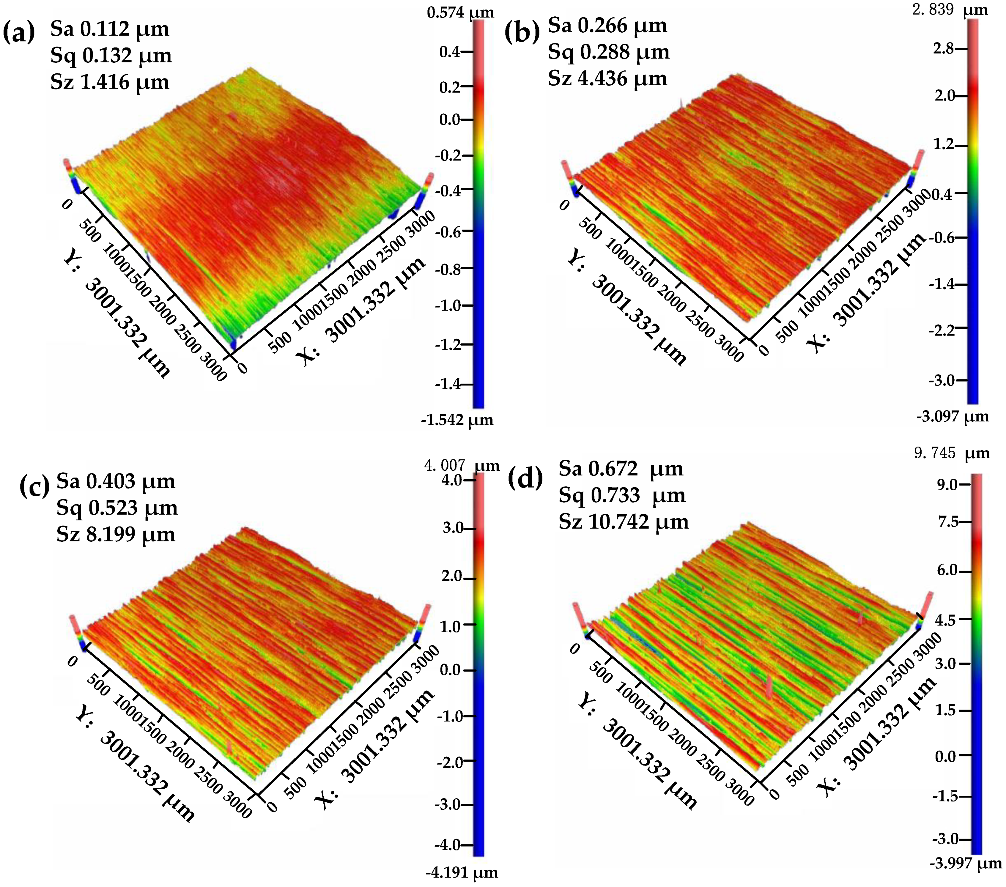
Figure 2.
The 2D power spectral density: (a) Surface 1; (b) Surface 2; (c) Surface 3; (d) Surface 4.
Figure 2.
The 2D power spectral density: (a) Surface 1; (b) Surface 2; (c) Surface 3; (d) Surface 4.
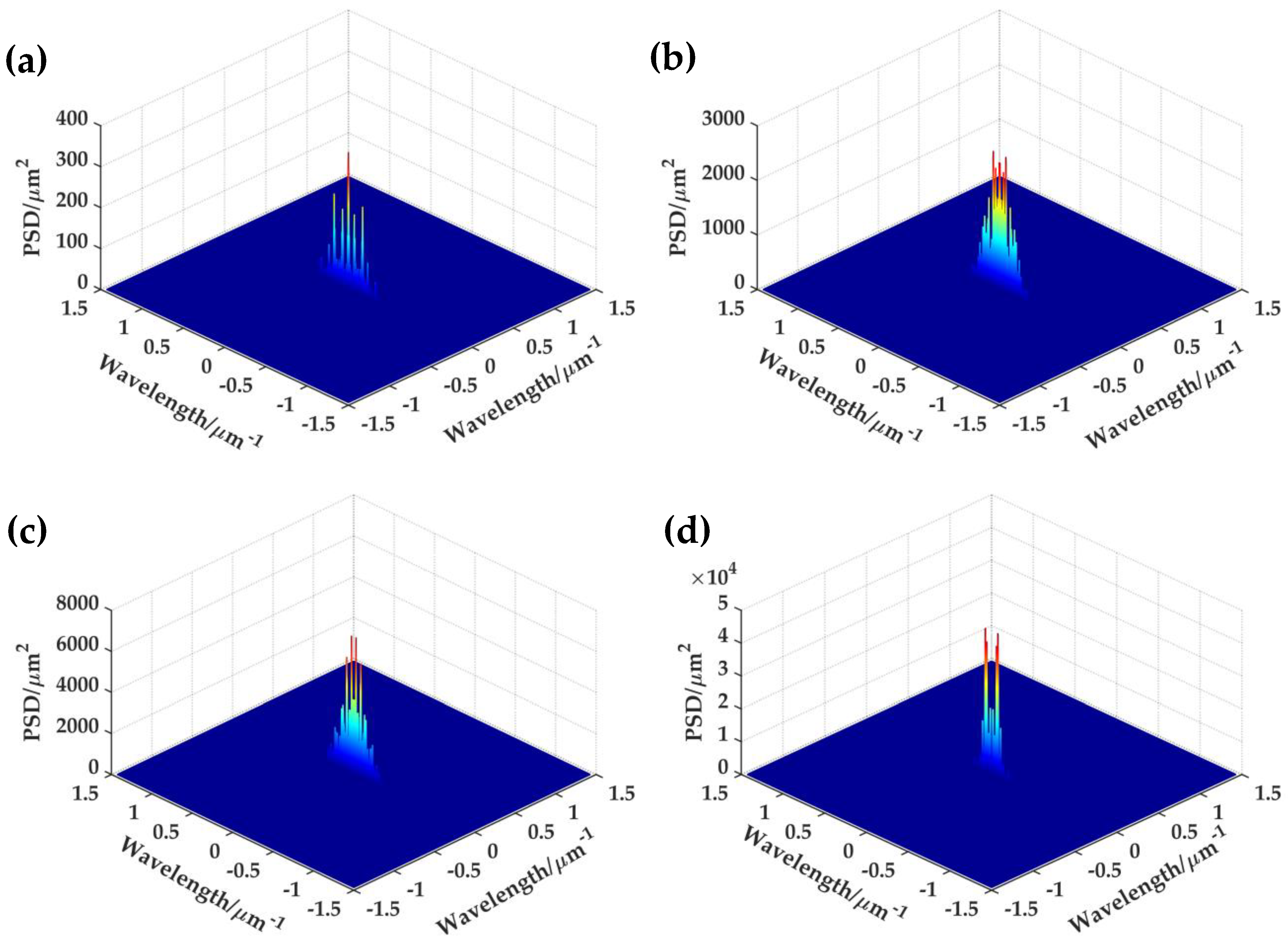
Figure 3.
The 3D fractal surfaces under D = 2.4, G = 1 × 10⁻¹³: (a) Isotropic surface; (b) anisotropic surface.
Figure 3.
The 3D fractal surfaces under D = 2.4, G = 1 × 10⁻¹³: (a) Isotropic surface; (b) anisotropic surface.
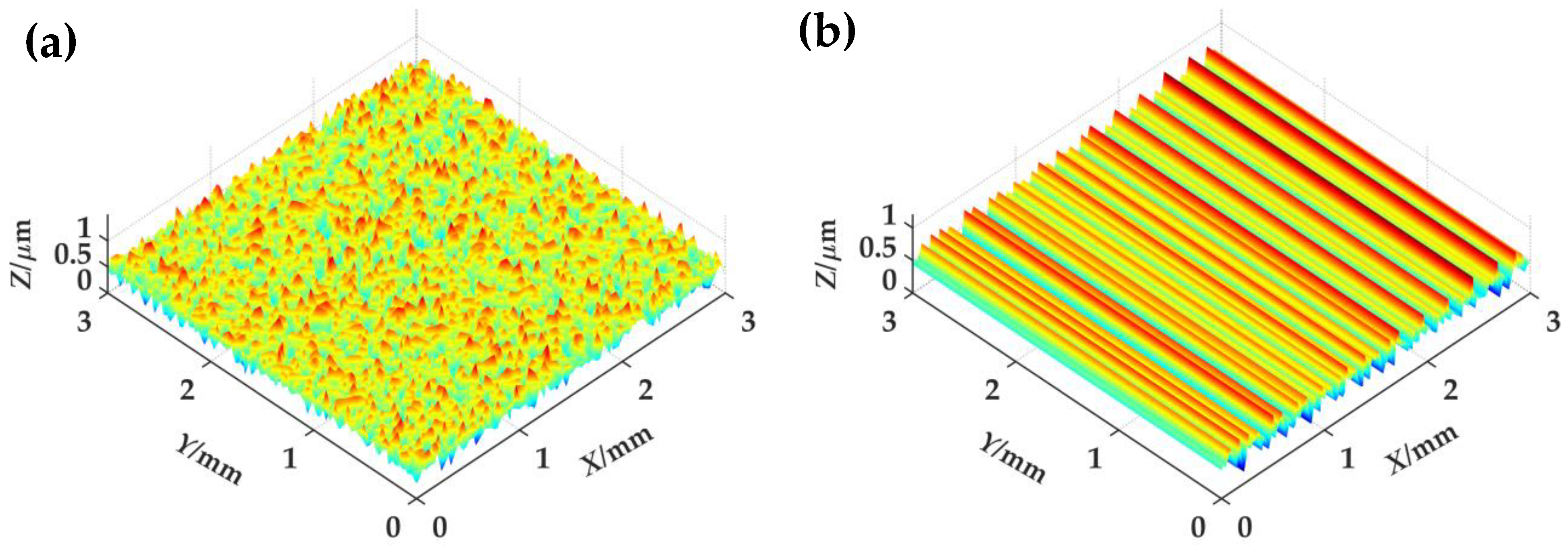
Figure 4.
The ubiquitiformal surfaces under different δmin: (a) δmin = 10−3 m; (b) δmin = 10−5 m; (c) δmin = 10−7 m; (d) δmin = 10−9 m.
Figure 4.
The ubiquitiformal surfaces under different δmin: (a) δmin = 10−3 m; (b) δmin = 10−5 m; (c) δmin = 10−7 m; (d) δmin = 10−9 m.

Figure 5.
Fractal surfaces: (a) Surface 1; (b) Surface 2; (c) Surface 3; (d) Surface 4.
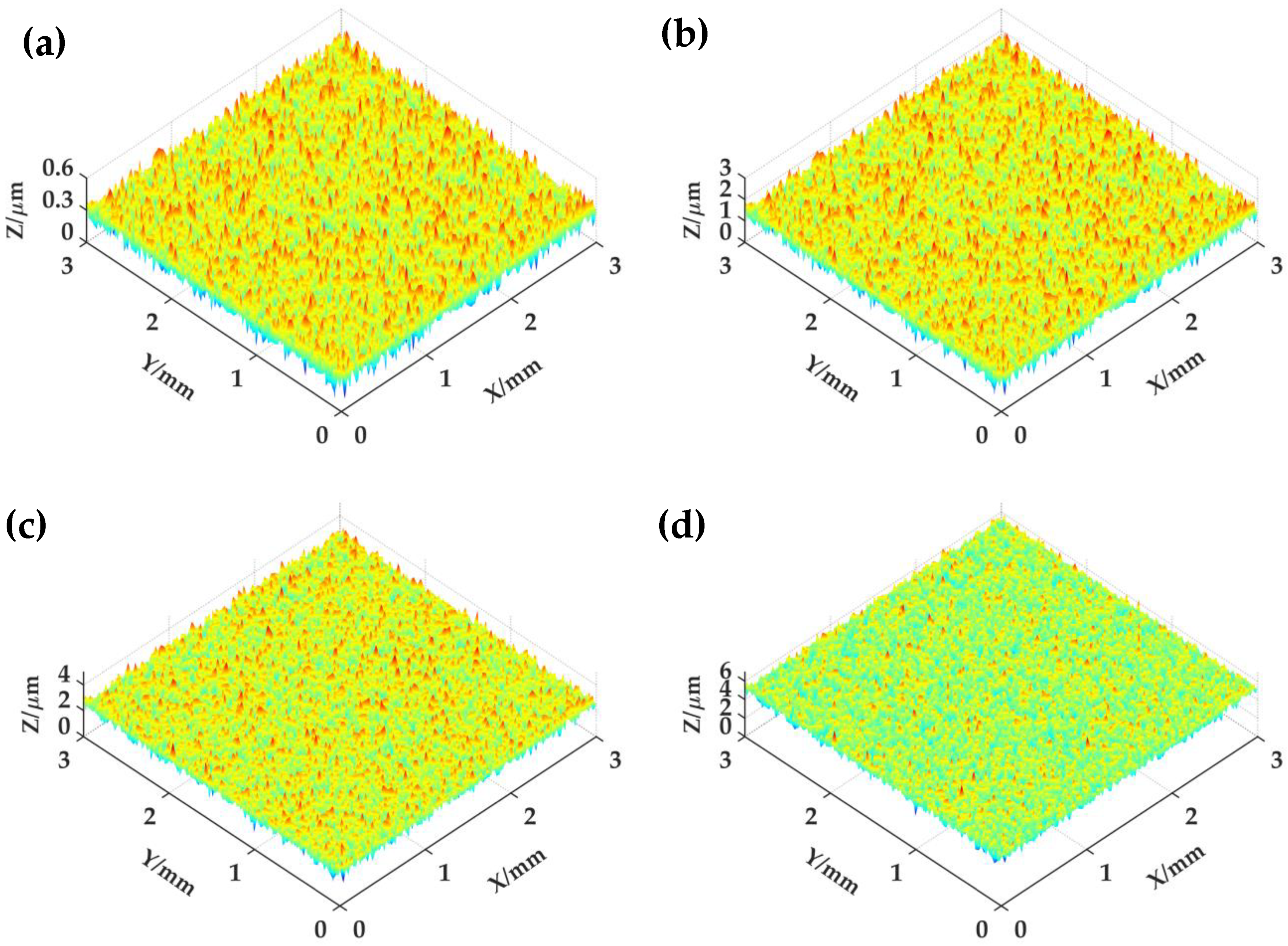
Figure 6.
Ubiquitiformal surfaces: (a) Surface 1; (b) Surface 2; (c) Surface 3; (d) Surface 4.
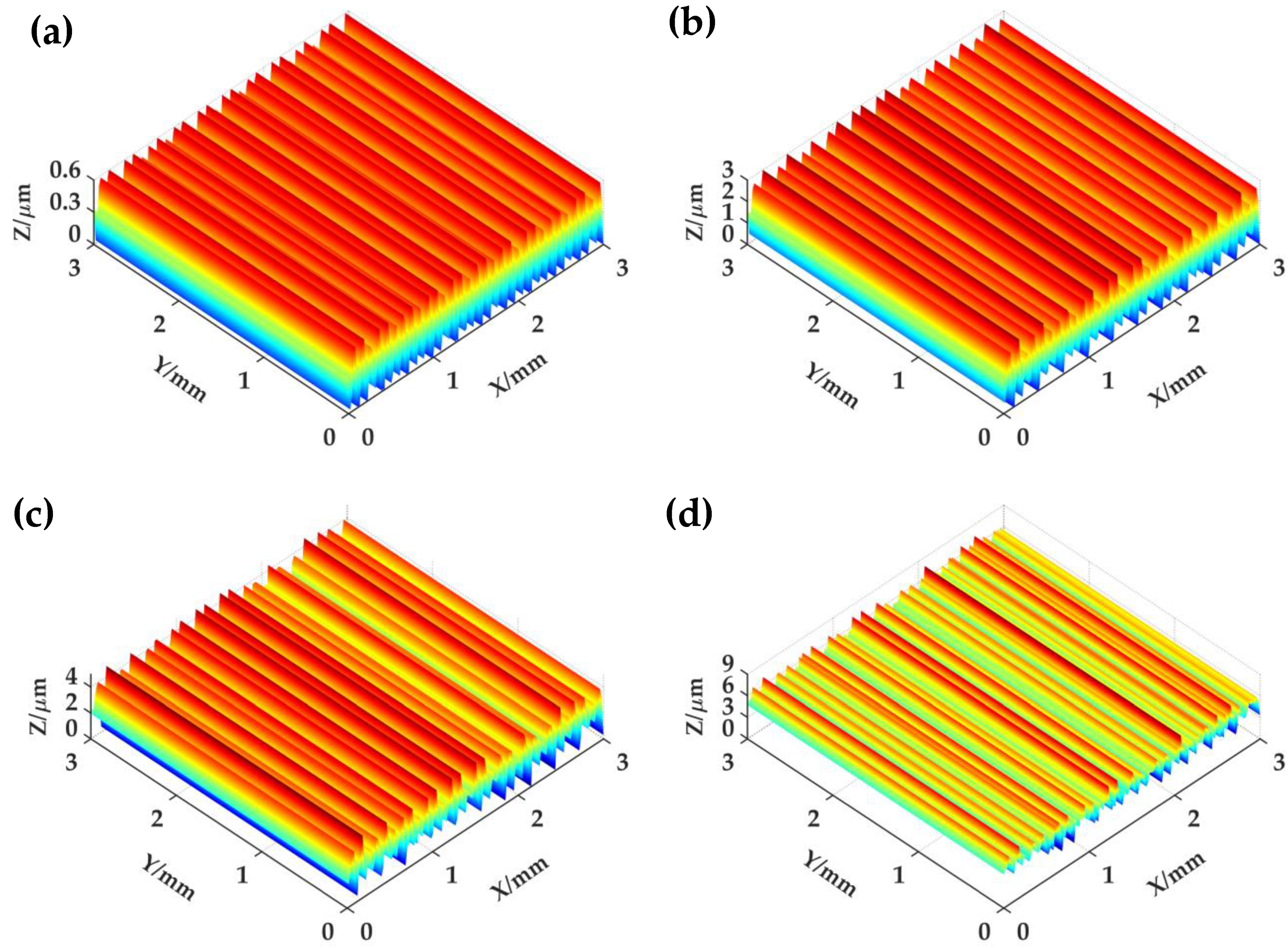
Figure 7.
The relative errors of roughness parameters under different δmin: (a) Sa; (b) Sq; (c) Ssk; (d) Sku.
Figure 7.
The relative errors of roughness parameters under different δmin: (a) Sa; (b) Sq; (c) Ssk; (d) Sku.
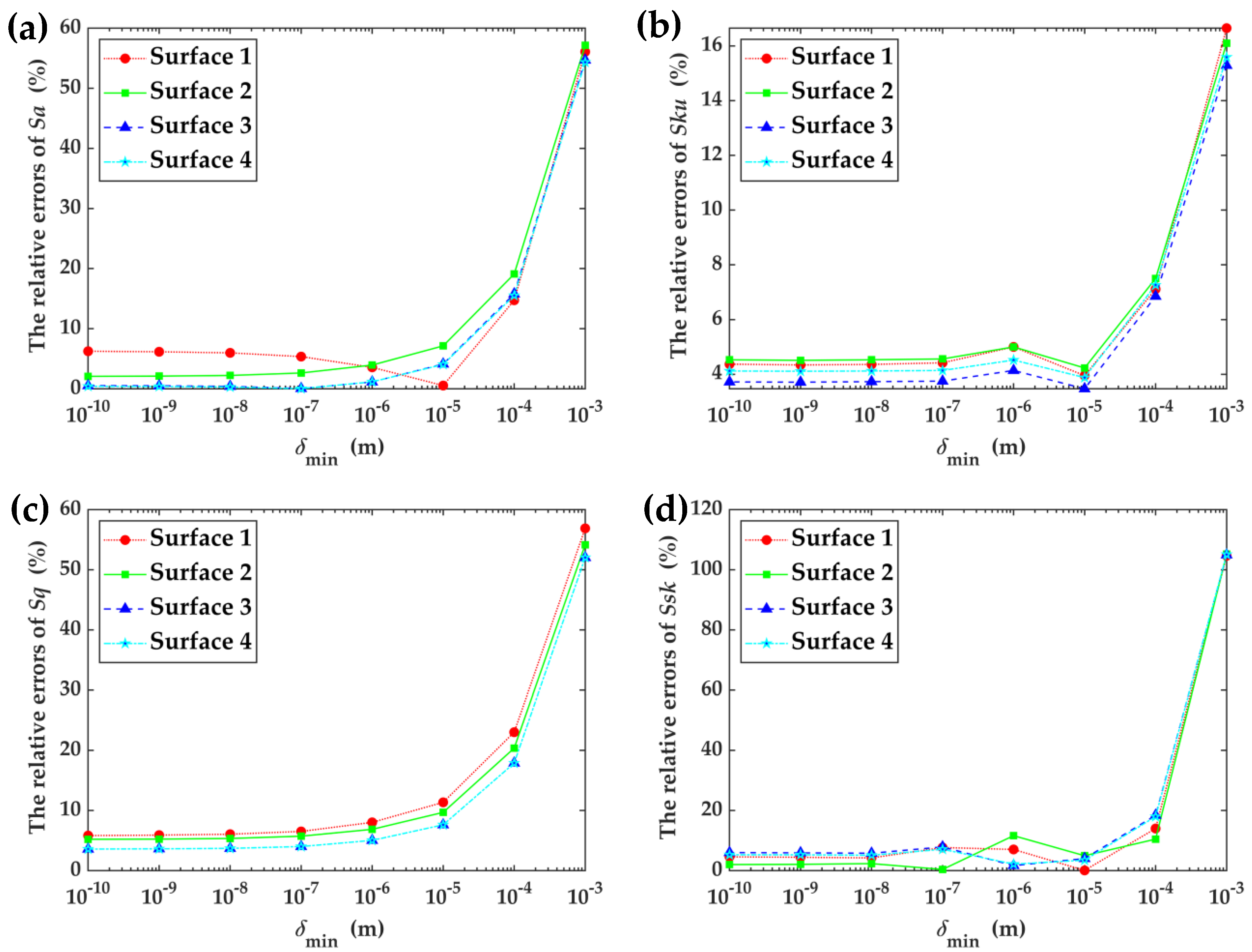
Figure 8.
The relative errors of roughness parameters under different modeling methods: (a) Surface 1; (b) Surface 2; (c) Surface 3; (d) Surface 4.
Figure 8.
The relative errors of roughness parameters under different modeling methods: (a) Surface 1; (b) Surface 2; (c) Surface 3; (d) Surface 4.

Table 1.
The fractal characteristic parameters of different grinding surfaces.
| Fractal Characteristic Parameters | Surface 1 | Surface 2 | Surface 3 | Surface 4 |
|---|---|---|---|---|
| D | 2.553 | 2.517 | 2.497 | 2.491 |
| G | 5.279 × 10⁻¹² | 6.761 × 10⁻¹² | 7.939 × 10⁻¹² | 1.802 × 10⁻¹¹ |
Publisher’s Note: MDPI stays neutral with regard to jurisdictional claims in published maps and institutional affiliations. |
© 2022 by the authors. Licensee MDPI, Basel, Switzerland. This article is an open access article distributed under the terms and conditions of the Creative Commons Attribution (CC BY) license (https://creativecommons.org/licenses/by/4.0/).
Share and Cite
MDPI and ACS Style
Liu, Y.; An, Q.; Huang, M.; Shang, D.; Bai, L. A Novel Modeling Method of Micro-Topography for Grinding Surface Based on Ubiquitiform Theory. Fractal Fract. 2022, 6, 341. https://doi.org/10.3390/fractalfract6060341
AMA Style
Liu Y, An Q, Huang M, Shang D, Bai L. A Novel Modeling Method of Micro-Topography for Grinding Surface Based on Ubiquitiform Theory. Fractal and Fractional. 2022; 6(6):341. https://doi.org/10.3390/fractalfract6060341
Chicago/Turabian StyleLiu, Yue, Qi An, Min Huang, Deyong Shang, and Long Bai. 2022. "A Novel Modeling Method of Micro-Topography for Grinding Surface Based on Ubiquitiform Theory" Fractal and Fractional 6, no. 6: 341. https://doi.org/10.3390/fractalfract6060341