
The Passivity of Uncertain Fractional-Order Neural Networks with Time-Varying Delays

1
Construction Economics and Real Estate Management Research Center, Anhui Jianzhu University, Hefei 230009, China
2
School of Mathematics and Physics, Guangxi Minzu University, Nanning 530006, China
3
School of Mathematics and Physics, China University of Geosciences, Wuhan 430074, China
*
Author to whom correspondence should be addressed.
Fractal Fract. 2022, 6(7), 375; https://doi.org/10.3390/fractalfract6070375
Submission received: 25 May 2022
/
Revised: 20 June 2022
/
Accepted: 28 June 2022
/
Published: 2 July 2022
(This article belongs to the Special Issue Robust and Adaptive Control of Fractional-Order Systems)
Abstract
:In this paper, we study the passive problem of uncertain fractional-order neural networks (UFONNs) with time-varying delays. First, we give a sufficient condition for the asymptotic stability of UFONNs with bounded time-varying delays by using the fractional-order Razumikhin theorem. Secondly, according to the above stability criteria and some properties of fractional-order calculus, a delay-dependent condition that can guarantee the passivity of UFONNs with time-varying delays is given in the form of a linear matrix inequality (LMI) that can be reasonably solved in polynomial time using the LMI Control Toolbox. These conditions are not only delay-dependent but also order-dependent, and less conservative than some existing work. Finally, the rationality of the research results is proved by simulation.
Keywords:
passivity analysis; time-varying delays; uncertain fractional-order neural network; asymptotically stableMSC:
47H09; 34A081. Introduction
As neural networks (NNs) play an important role in the field of control engineering and are used for applications such as association [1,2], pattern recognition [3,4], and signal processing [5,6], fractional-order neural networks (FONNs) are becoming more and more popular among scientists. Moreover, since two important properties of fractional-order calculus are memorability and heritability, FONNs can more precisely describe the dynamic behavior of neurons in NNs. Therefore, many problems related to FONNs have been studied, such as finite-time stability [7,8,9], asymptotic stability [10,11,12,13], synchronization analysis [14,15,16,17], and guaranteed cost control [18,19].
Passivity theory has been a major concern in the field of control engineering since the 1970s (see references [20,21,22,23,24]). As an effective tool for studying system stability, passivity theory has been applied to a variety of areas, for example, fuzzy control, complexity, power systems, and signal processing. Some researchers have also extended passivity theory to NNs. The passive filtering of NNs with time-varying mixed delays using the Wirtinger integral inequality was studied in [25]. Other research on the passivity of dynamic NNs can be found in the literature [26,27,28,29,30]. Although there are many research results on the passivity of NNs, the research on the passivity of NNs with time-varying delays has not been fully explored. At present, the passivity of integer-order NNs with time-varying delays has been studied using different methods. For example, in [31], Lyapunov–Krasovskii functions were used to analyze the stability and passivity of NNs with time-varying delays. The passivity of integer-order NNs with discrete and distributed time-varying delays was studied in [32]. By means of stochastic analysis and linear matrix inequality (LMI) techniques, event-triggered passive synchronization for NNs with random gain changes was addressed in [33]. More research on the passivity of neural networks with time delays can be found in [34,35,36]. In the above-mentioned research results, we find that the methods used to study passivity mainly used LMI techniques and Lyapunov–Krasovskii functions. The passive analysis of an integer-order system can be simplified by taking the integer derivative of a Lyapunov–Krasovskii function. However, constructing fractional-order Lyapunov–Krasovskii functions for FONNs is challenging due to the limitation of integral intervals. In other words, the method mentioned above cannot be extended to the study of the passivity of FONNs with time-varying delays. The question of how to solve this problem is interesting and challenging.
It is well known that fractional derivatives have weak singular kernels and are nonlocal. Therefore, compared with integer-order NNs, the passive research of FONNs is more challenging. Up to now, there have only been very few works that considered passivity [37,38]. In [37], the authors studied the passive problem of FONNs by means of an LMI technique and control theory; only the order-independent case was studied, and time delays were not considered. However, time delays are very common in all kinds of systems, and their existence can lead to system instability and transient responses. When the delay is small, the delay-independent stability condition is less conservative. Very recently, the passivity of FONNs with time-varying delays was studied using an LMI technique and control theory in [38], where system uncertainties were not considered. However, the connection weight of a neuron depends on its capacitance and resistance values, including uncertainties, so it is very important to study the passivity of uncertain fractional-order neural networks (UFONNs).
Based on the above analysis, in this article, our main task is to find a relatively simple order-dependent and delay-dependent condition for the passive problem of UFONNs with time-varying delays. The innovations of this article are as follows. (1) A relatively small conservative order-dependent and delay-dependent stability criterion for UFONNs with time-varying delays is presented using LMI techniques and the fractional-order Razumikhin theorem. (2) Based on fractional-order calculus and existing stability criteria, we solve the passive problem of UFONNs with time-varying delays. (3) Two sufficient conditions for UFONNs with passive time-varying delays are shown using an LMI. Furthermore, these conditions can be reasonably solved.
The rest of this article is divided into the following parts. In Section 2, we detail some assumptions, definitions, and lemmas and describe the research object of this article. In Section 3, the passive study of UFONNs with time-varying delays is presented. A simulation example is used to prove the rationality of the theoretical results in Section 4.
Notations: In this article, is defined as an n-dimensional Euclidean space, and is an appropriately dimensional identity matrix. is defined as the set of matrices, stands for the transpose of the matrix , and represents the block-diagonal matrix. is defined as the whole function on the interval , in which the first-order derivative of any function exists and is continuous. is a space of all 2-integrable functions on . is a segment of trajectory . For convenience, we use ∗ to replace the symmetric term in the symmetric matrix.
2. Preliminaries
The -th Caputo fractional-order integral is given as:
where .
The -th Caputo fractional differential is given as:
where . In addition, for the sake of convenience, we only consider .
That yields the following UFONNs:
where is the neuron state vector, is a positive diagonal matrix, , are interconnection weight matrices, is the time delay, and is a known constant matrix. is the input vector; and are unknown matrices representing the uncertainties of time-varying parameters; represents the neural activation function; and is output vector. is the initial vector value function.
Remark 1.
In engineering applications and real-world systems, parameters often fluctuate within certain ranges, which can lead to divergence or instability. Thus, it makes sense to introduce parameter uncertainty into fractional-order neural networks; doing so can reveal more realistic dynamic properties of fractional-order neural networks. The passive theory can maintain the internal stability of the system, which plays an important role in network control theory. It also has a wide range of applications in robotic systems, electromechanical systems, power systems, internal combustion engine engineering, and chemical processes. Therefore, studying the passivity of uncertain fractional-order neural networks provides an important theoretical basis for engineering applications.
The following are the relevant lemmas, definitions, and assumptions.
Assumption 1.
The activation function satisfies for any :
where , are known constants.
Remark 2.
Note that and can be any real number, and that is a much broader set of conditions than the Lipschitz-type activation functions.
Assumption 2.
, , are defined by:
where and are unknown time-varying matrices, and and are known constant matrices with appropriate dimensions and satisfy:
Lemma 1 ([39]).
If for some , then for , we have:
and:
Lemma 2 ([40]).
If is a continuous function, then:
Lemma 3 ([40]).
Caputo’s fractional-order calculus satisfies:
where λ, .
Lemma 4 ([39]).
If function is differentiable, then there is a symmetric positive definite matrix such that:
Lemma 5 ([41]).
If there are three positive constants and and a quadratic Lyapunov function that satisfies:
- (1)
- ,
- (2)
- whenever and for some , then the zero solution of system is asymptotically stable.
Remark 3.
In fact, there is a connection between passivity and stability. If the system is passive, then we find that the system is asymptotically stable with zero output vectors and zero external input vectors, as can be seen in [30]. In addition, our Definition 1 is equivalent to an expansion of the definition in [42]. If the system satisfies both (1) and (2) in Definition 1, then the system must be passive. and in Definition 1 are consistent with those given by System (3).
3. Main Results
3.1. Stability Study of the System
In this part, the stability of System (3) with and is analyzed. First, let us emphasize that for the sake of our calculations, in Theorems 1 and 2, the following substitutions are made: to represent , to represent , to represent , means , and represents .
Theorem 1.
Assuming that Assumptions 1 and 2 are true, System (3) with and is asymptotically stable if there exist symmetric positive definite matrices and , a symmetric semi-positive definite matrix , and three positive diagonal matrices such that:
where:
,
,
,
,
,
,
,
,
,
,
, .
Proof.
Let us choose the Lyapunov function:
and it satisfies:
Therefore, condition of Lemma 5 is satisfied. Then, by taking the -th fractional derivative of the above , we have:
For any symmetric positive definite matrix and any symmetric semi-positive definite matrix , the following formulae can be obtained:
and:
where .
For Assumption 1, we know that for any , we obtain:
It is equivalent to:
For Assumption 2, we derive that for any , one obtains:
For Lemma 5, we assume that yields:
which implies:
Because is any parameter that is greater than 1, we take for (23), and we have:
So (25) is equivalent to:
Since , we obtain:
where .
Therefore, when , it implies that . So, this satisfies condition of Lemma 5. Finally, System (3) is asymptotically stable when both the output and the external input are zero. □
Remark 4.
At present, the LMI technique is widely used to research the stability of various FONNs with time-varying delays. Its greatest advantage is that we can use convex algorithms to solve it reasonably in polynomial time.
3.2. Passivity Analysis of the System
In the following, the passivity of System (3) is analyzed.
Theorem 2.
Assuming that Assumptions 1 and 2 are true, if there exist symmetric positive definite matrices and , a symmetric semi-positive definite matrix , three positive diagonal matrices , and such that:
where
,
,
,
,
,
,
,
,
,
,
, ,
Proof.
To facilitate the treatment of the passivity of System (3), we use in Theorem 1. By using the same method that we used to prove Theorem 1, we obtain an estimate:
in which . From (28), we have:
The integral of Inequality (30) is given as:
Because of , thus:
Therefore, System (3) is passive and can be obtained using Definition 1 and Theorem 1. □
Remark 5.
It is well known that the time-delay dependent condition is less conservative than the time-delay independent condition because it takes into account time delay information. In [43], the authors derived a time-delay dependent stability criterion, but it is worth noting that this sufficient condition considers systems with constant time delay. In [37], the authors obtained an order-independent passive analysis criterion, whereas we obtained an order-dependent and delay-dependent passive analysis criterion; thus, the results we obtained in Theorems 1 and 2 are less conservative than those in [37,43,44].
Remark 6.
From Definition 1, we can see that if we want to prove that System (3) is passive, then first we need to show that System (3) is asymptotically stable with and , then prove that System (3) satisfies the definition of passivity with zero initial conditions. Therefore, from Definition 1 combined with the proofs of Theorems 1 and 2 in this paper, we know that Theorem 2 is based on the establishment of Theorem 1; thus, we see that matrix Λ in Theorem 1 is a submatrix of matrix Σ in Theorem 2.
Remark 7.
The passivity of NNs has been the focus of many research papers. For example, in [29], the robust finite-time passivity of UFONNs was studied, but the passivity of the system when time delays existed was not considered. In [38], the passivity of FONNs with time-varying delays was studied, but the uncertainties were not considered. In [45], the passivity of FONNs with time-varying parameter uncertainties was studied. However, the author used a sufficient condition that guaranteed the system was passive, independent of the order of the system. As far as we know, there exists no report on the passivity of UFONNs with time-varying delays. For this article, we use the method of [38] to deduce the order-dependent and delay-dependent passivity conditions for making the system passive by means of the definition of passivity and the Razumikhin theorem. Compared with the method of constructing Lyapunov–Krasovskii functions used in the existing literature, our method is simpler and less conservative.
4. Simulation Examples
Below, the correctness of the theoretical results is confirmed by simulation experiments.
Example 1.
Given the following UFONNs:
where is the state variable of the NNs, is the output, and is the external input of System (33). The parameter matrices are , , , and . Define the uncertainties as follows: , , , , , and .
Obviously, these uncertainties satisfy Assumption 2. The time delay is . The activation function is . Based on Assumption 1, we obtain , and . Using Theorem 1, the feasible solutions for the LMI (13) are , , , , ,
where
, ,
, ,
, ,
, ,
, ,
, ,
, ,
, ,
, ,
, ,
, ,
, ,
, ,
, ,
,
and , which means that when and , the UFONNs with time-varying delays are asymptotically stable in the sense of Definition 1 and Theorem 1. From Theorem 2, we find that , so System (33) is passive. The passive parameter ρ obtained in the simulation example is only the value when the order of System (33) is . In addition, we take the different order β of System (33) to analyze its relationship with the passive parameter ρ in Table 1.
5. Conclusions
In this paper, by means of knowledge of fractional-order calculus and the fractional-order Razumikhin theorem, the passivity of UFONNs with time-varying delays was studied. It was proved that UFONNs with time-varying delays are asymptotically stable when both the output and the external input are zero, and when the delay-dependent and order-dependent LMI is satisfied. In addition, based on the proof of asymptotic stability, UFONNs with time-varying delays are passive when they contain a nonzero external input vector and output vector. In the future, we will study the passive problem of UFONNs, including unbounded time-varying time delays and multiple time delays.
Author Contributions
S.X.: investigation, writing—review and editing; H.L.: conceptualization, supervision; Z.H.: methodology, writing—original draft. All authors have read and agreed to the published version of the manuscript.
Funding
This work was supported by the Key Research Projects of Humanties and Social Sciences in Anhui Universities (SK2021A0346) and the Anhui Jianzhu University Research Startup Project (2019QDZ61).
Institutional Review Board Statement
Not applicable.
Informed Consent Statement
Informed consent was obtained from all subjects involved in the study.
Data Availability Statement
All data included in this study are available upon request via contact with the corresponding author.
Conflicts of Interest
The authors declare no conflict of interest.
References
- Kolachalama, V.B.; Singh, P.; Lin, C.Q.; Mun, D.; Belghasem, M.E.; Henderson, J.M.; Francis, J.M.; Salant, D.J.; Chitalia, V.C. Association of pathological fibrosis with renal survival using deep neural networks. Kidney Int. Rep. 2018, 3, 464–475. [Google Scholar] [CrossRef] [PubMed] [Green Version]
- Peng, J.; Hui, W.; Li, Q.; Chen, B.; Hao, J.; Jiang, Q.; Shang, X.; Wei, Z. A learning-based framework for miRNA-disease association identification using neural networks. Bioinformatics 2019, 35, 4364–4371. [Google Scholar] [CrossRef] [PubMed] [Green Version]
- Cherry, K.M.; Qian, L. Scaling up molecular pattern recognition with DNA-based winner-take-all neural networks. Nature 2018, 559, 370–376. [Google Scholar] [CrossRef] [PubMed]
- Kong, Q.; Cao, Y.; Iqbal, T.; Wang, Y.; Wang, W.; Plumbley, M.D. Panns: Large-scale pretrained audio neural networks for audio pattern recognition. IEEE/ACM Trans Audio Speech Lang. Process. 2020, 28, 2880–2894. [Google Scholar] [CrossRef]
- Sainath, T.N.; Weiss, R.J.; Wilson, K.W.; Li, B.; Narayanan, A.; Variani, E.; Bacchiani, M.; Shafran, I.; Senior, A.; Chin, K.; et al. Multichannel signal processing with deep neural networks for automatic speech recognition. IEEE/ACM Trans. Audio Speech Lang. Process. 2017, 25, 965–979. [Google Scholar] [CrossRef]
- Pelenis, D.; Barauskas, D.; Vanagas, G.; Dzikaras, M.; Viržonis, D. CMUT-based biosensor with convolutional neural network signal processing. Ultrasonics 2019, 99, 105956. [Google Scholar] [CrossRef]
- Xu, C.J.; Li, P.L. On Finite-Time Stability for Fractional-Order Neural Networks with Proportional Delays. Neural Process. Lett. 2019, 50, 1241–1256. [Google Scholar] [CrossRef]
- Saravanakumar, R.; Stojanovic, S.B.; Radosavljevic, D.D.; Ahn, C.K.; Karimi, H.R. Finite-Time Passivity-Based Stability Criteria for Delayed Discrete-Time Neural Networks via New Weighted Summation Inequalities. IEEE Trans. Neural Networks Learn. Syst. 2018, 30, 58–71. [Google Scholar] [CrossRef]
- Pratap, A.; Raja, R.; Alzabut, J.; Dianavinnarasi, J.; Rajchakit, G. Finite-time Mittag-Leffler stability of fractional-order quaternion-valued memristive neural networks with impulses. Neural Process. Lett. 2020, 51, 1485–1526. [Google Scholar] [CrossRef]
- Wu, Z. Multiple asymptotic stability of fractional-order quaternion-valued neural networks with time-varying delays. Neurocomputing 2021, 448, 301–312. [Google Scholar] [CrossRef]
- Li, J.D.; Wu, Z.B.; Huang, N.J. Asymptotical stability of Riemann-Liouville fractional-order neutral-type delayed projective neural networks. Neural Process. Lett. 2019, 50, 565–579. [Google Scholar] [CrossRef]
- Wang, F.; Yang, Y.; Xu, X.; Li, L. Global asymptotic stability of impulsive fractional-order BAM neural networks with time delay. Neural Comput. Appl. 2017, 28, 345–352. [Google Scholar] [CrossRef]
- Liu, H.; Li, S.; Wang, H.; Sun, Y. Adaptive Fuzzy Control for a Class of Unknown Fractional-Order Neural Networks Subject to Input Nonlinearities and Dead-Zones. Inf. Sci. 2018, 454, 30–45. [Google Scholar] [CrossRef]
- Yang, X.; Li, C.; Huang, T.; Song, Q.; Huang, J. Synchronization of fractional-order memristor-based complex-valued neural networks with uncertain parameters and time delays. Chaos Solitons Fractals 2018, 110, 105–123. [Google Scholar] [CrossRef]
- Huang, X.; Fan, Y.; Jia, J.; Wang, Z.; Li, Y. Quasi-synchronization of fractional-order memristor-based neural networks with parameter mismatches. IET Control. Theory Appl. 2017, 11, 2317–2327. [Google Scholar] [CrossRef]
- Zhang, W.; Cao, J.; Chen, D.; Fuad, A. Synchronization in Fractional-Order Complex-Valued Delayed Neural Networks. Entropy 2018, 20, 54. [Google Scholar] [CrossRef] [PubMed] [Green Version]
- Han, Z.; Li, S.; Liu, H. Composite learning sliding mode synchronization of chaotic fractional-order neural networks. J. Adv. Res. 2020, 25, 87–96. [Google Scholar] [CrossRef]
- Thuan, M.V.; Huong, D.C. Robust guaranteed cost control for time-delay fractional-order neural networks systems. Optim. Control. Appl. Methods 2019, 40, 613–625. [Google Scholar] [CrossRef]
- Thuan, M.V.; Binh, T.N.; Huong, D.C. Finite-time guaranteed cost control of Caputo fractional-order neural networks. Asian J. Control. 2020, 22, 696–705. [Google Scholar] [CrossRef]
- Li, F.; Du, C.; Yang, C.; Gui, W. Passivity-based asynchronous sliding mode control for delayed singular Markovian jump systems. IEEE Trans. Autom. Control. 2017, 63, 2715–2721. [Google Scholar] [CrossRef]
- Zhang, M.; Borja, P.; Ortega, R.; Liu, Z.; Su, H. PID passivity-based control of port-Hamiltonian systems. IEEE Trans. Autom. Control. 2017, 63, 1032–1044. [Google Scholar] [CrossRef]
- Yang, B.; Yu, T.; Shu, H.; Zhang, Y.; Chen, J.; Sang, Y.; Jiang, L. Passivity-based sliding-mode control design for optimal power extraction of a PMSG based variable speed wind turbine. Renew. Energy 2018, 119, 577–589. [Google Scholar] [CrossRef]
- Ramos, E.R.; Leyva, R.; Farivar, G.G.; Tafti, H.D.; Townsend, C.D.; Pou, J. Incremental passivity control in multilevel cascaded H-bridge converters. IEEE Trans. Power Electron. 2020, 35, 8766–8778. [Google Scholar] [CrossRef]
- Mehrasa, M.; Babaie, M.; Zafari, A.; Al-Haddad, K. Passivity ANFIS-based control for an intelligent compact multilevel converter. IEEE Trans. Ind. Inform. 2021, 17, 5141–5151. [Google Scholar] [CrossRef]
- Zhang, X.; Fan, X.F.; Xue, Y.; Wang, Y.T.; Cai, W. Robust exponential passive filtering for uncertain neutral-type neural networks with time-varying mixed delays via Wirtinger-based integral inequality. Int. J. Control. Autom. Syst. 2017, 15, 585–594. [Google Scholar] [CrossRef]
- Xiao, Q.; Huang, T.; Zeng, Z. Passivity and passification of fuzzy memristive inertial neural networks on time scales. IEEE Trans. Fuzzy Syst. 2018, 26, 3342–3355. [Google Scholar] [CrossRef]
- Huang, C.; Wang, W.; Cao, J.; Lu, J. Synchronization-based passivity of partially coupled neural networks with event-triggered communication. Neurocomputing 2018, 319, 134–143. [Google Scholar] [CrossRef]
- Zhang, R.; Bilige, S.; Chaolu, T. Fractal solitons, arbitrary function solutions, exact periodic wave and breathers for a nonlinear partial differential equation by using bilinear neural network method. J. Syst. Sci. Complex. 2021, 34, 122–139. [Google Scholar] [CrossRef]
- Thuan, M.V.; Huong, D.C.; Hong, D.T. New results on robust finite-time passivity for fractional-order neural networks with uncertainties. Neural Process. Lett. 2019, 50, 1065–1078. [Google Scholar] [CrossRef]
- Rajchakit, G.; Sriraman, R. Robust passivity and stability analysis of uncertain complex-valued impulsive neural networks with time-varying delays. Neural Process. Lett. 2021, 53, 581–606. [Google Scholar] [CrossRef]
- Park, M.J.; Kwon, O.M.; Ryu, J.H. Passivity and stability analysis of neural networks with time-varying delays via extended free-weighting matrices integral inequality. Neural Netw. 2018, 106, 67–78. [Google Scholar] [CrossRef]
- Ge, C.; Ju, H.P.; Hua, C.; Shi, C. Robust passivity analysis for uncertain neural networks with discrete and distributed time-varying delays. Neurocomputing 2019, 364, 330–337. [Google Scholar] [CrossRef]
- Dai, M.; Xia, J.; Xia, H.; Shen, H. Event-triggered passive synchronization for Markov jump neural networks subject to randomly occurring gain variations. Neurocomputing 2019, 331, 403–411. [Google Scholar] [CrossRef]
- Chen, Y.; Wang, H.; Xue, A.; Lu, R. Passivity analysis of stochastic time-delay neural networks. Nonlinear Dyn. 2010, 61, 71–82. [Google Scholar] [CrossRef]
- Li, N.; Cao, J. Passivity and robust synchronisation of switched interval coupled neural networks with time delay. Int. J. Syst. Sci. 2016, 47, 2827–2836. [Google Scholar] [CrossRef]
- Zhang, X.; Han, Q.; Ge, X.; Zhang, B. Passivity analysis of delayed neural networks based on Lyapunov-Krasovskii functionals with delay-dependent matrices. IEEE Trans. Cybern. 2018, 50, 946–956. [Google Scholar] [CrossRef]
- Ding, Z.; Zeng, Z.; Zhang, H.; Wang, L.; Wang, L. New results on passivity of fractional-order uncertain neural networks. Neurocomputing 2019, 351, 51–59. [Google Scholar] [CrossRef]
- Sau, N.H.; Mai, V.T.; Huyen, N. Passivity analysis of fractional-order neural networks with time-varying delay based on LMI approach. Circuits Syst. Signal Process. 2020, 39, 5906–5925. [Google Scholar] [CrossRef]
- Liu, H.; Pan, Y.; Li, S.; Ye, C. Adaptive Fuzzy Backstepping Control of Fractional-Order Nonlinear Systems. IEEE Trans. Syst. Man Cybern. Syst. 2017, 47, 2209–2217. [Google Scholar] [CrossRef]
- Kilbas, A.; Srivastava, H.M.; Trujillo, J.J. Theory and Applications of Fractional Differential Equations; Elsevier: Amsterdam, The Netherlands, 2006. [Google Scholar]
- Liu, S.; Yang, R.; Zhou, X.F.; Jiang, W.; Li, X.; Zhao, X.W. Stability analysis of fractional delayed equations and its applications on consensus of multi-agent systems. Commun. Nonlinear Sci. Numer. Simul. 2019, 73, 351–362. [Google Scholar] [CrossRef]
- Zhang, Z.; Mou, S.; Lam, J.; Gao, H. New passivity criteria for neural networks with time-varying delay. Neural Netw. 2009, 22, 864–868. [Google Scholar] [CrossRef]
- Yang, Y.; He, Y.; Wang, Y.; Wu, M. Stability analysis of fractional-order neural networks: An LMI approach. Neurocomputing 2018, 285, 82–93. [Google Scholar] [CrossRef]
- Chen, L.; Chai, Y.; Wu, R.; Zhai, H. Dynamic analysis of a class of fractional-order neural networks with delay. Neurocomputing 2013, 111, 190–194. [Google Scholar] [CrossRef]
- Ding, Z. Passivity analysis of fractional-order neural networks with time-varying parameter uncertainties. In Proceedings of the 2018 Chinese Automation Congress (CAC), Xi’an, China, 30 November–2 December 2018; pp. 265–268. [Google Scholar]
Figure 1.
State dynamics of UFONNs with external input.
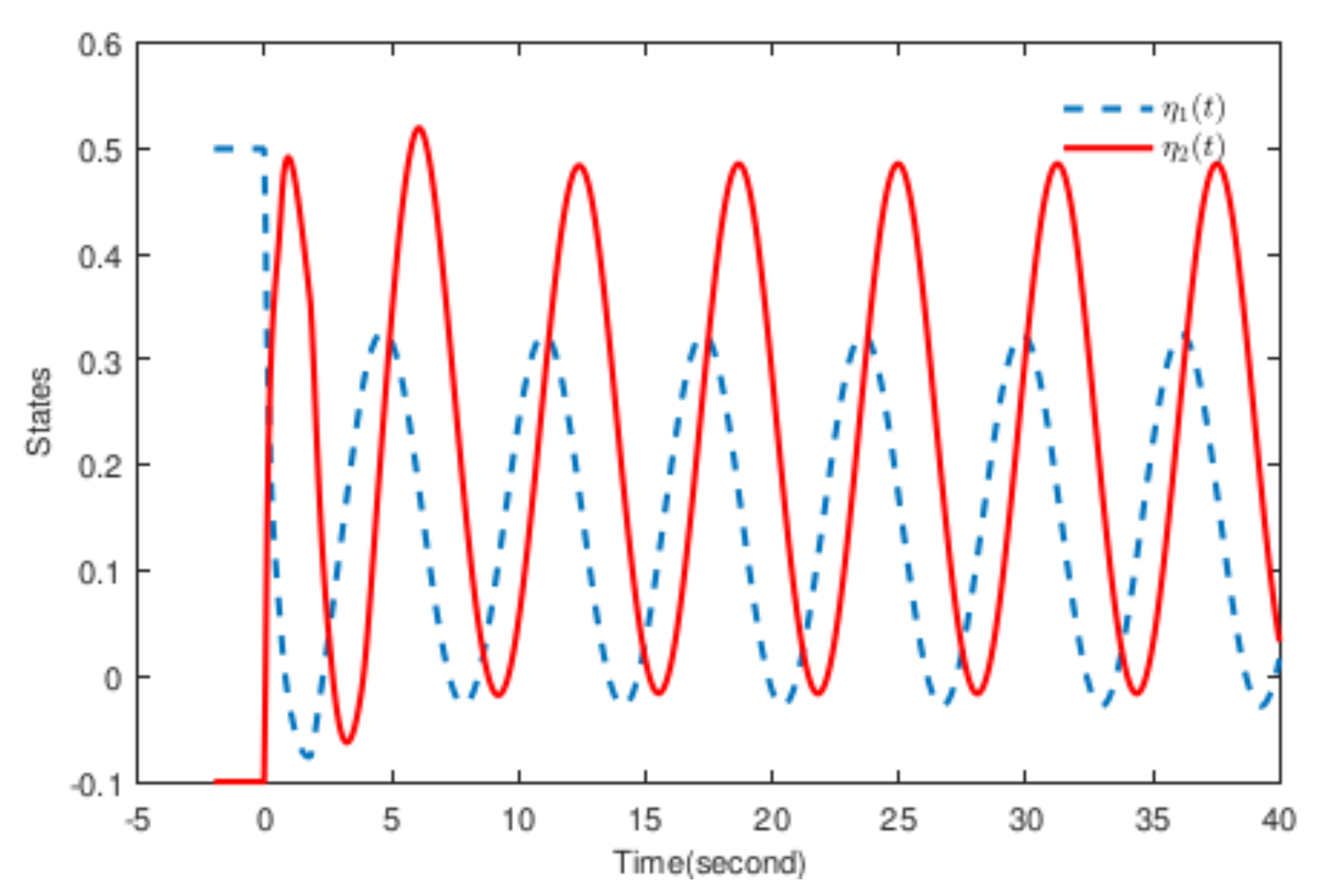
Figure 2.
State dynamics of UFONNs.
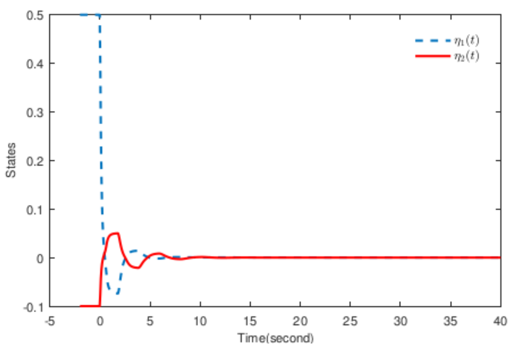
Figure 3.
State dynamics of UFONNs.


Table 1.
The relationship between the order of the system and the passive parameter in Theorem 2.
| The Order | The Passive Parameter |
|---|---|
| 0.1 | |
| 0.2 | 180.3959 |
| 0.3 | 248.7765 |
| 0.4 | 334.8487 |
| 0.5 | 357.8057 |
| 0.6 | 1.6010 |
| 0.7 | 20.5273 |
| 0.8 | 20.3400 |
| 0.9 | 22.4595 |
| 1 | 22.4947 |
Publisher’s Note: MDPI stays neutral with regard to jurisdictional claims in published maps and institutional affiliations. |
© 2022 by the authors. Licensee MDPI, Basel, Switzerland. This article is an open access article distributed under the terms and conditions of the Creative Commons Attribution (CC BY) license (https://creativecommons.org/licenses/by/4.0/).
Share and Cite
MDPI and ACS Style
Xu, S.; Liu, H.; Han, Z. The Passivity of Uncertain Fractional-Order Neural Networks with Time-Varying Delays. Fractal Fract. 2022, 6, 375. https://doi.org/10.3390/fractalfract6070375
AMA Style
Xu S, Liu H, Han Z. The Passivity of Uncertain Fractional-Order Neural Networks with Time-Varying Delays. Fractal and Fractional. 2022; 6(7):375. https://doi.org/10.3390/fractalfract6070375
Chicago/Turabian StyleXu, Song, Heng Liu, and Zhimin Han. 2022. "The Passivity of Uncertain Fractional-Order Neural Networks with Time-Varying Delays" Fractal and Fractional 6, no. 7: 375. https://doi.org/10.3390/fractalfract6070375