

A Mixed Finite Volume Element Method for Time-Fractional Damping Beam Vibration Problem
School of Mathematics and Statistics, Shandong Normal University, Jinan 250358, China
*
Author to whom correspondence should be addressed.
†
These authors contributed equally to this work.
Fractal Fract. 2022, 6(9), 523; https://doi.org/10.3390/fractalfract6090523
Submission received: 2 August 2022
/
Revised: 25 August 2022
/
Accepted: 10 September 2022
/
Published: 16 September 2022
(This article belongs to the Special Issue Fractional Diffusion Equations: Numerical Analysis, Modeling and Application)
Abstract
:In this paper, the transverse vibration of a fractional viscoelastic beam is studied based on the fractional calculus, and the corresponding scheme of a viscoelastic beam is established by using the mixed finite volume element method. The stability and convergence of the algorithm are analyzed. Numerical examples demonstrate the effectiveness of the algorithm. Finally, the values of different parameter sets are tested, and the test results show that both the damping coefficient and the fractional derivative have significant effects on the model. The results of this paper can be used for the damping modeling of viscoelastic structures.
Keywords:
time-fractional damping beam; vibration equation; mixed finite volume element method; stability; convergence; numerical simulationMSC:
65M08; 65M60; 34A08; 70J351. Introduction
According to the definition of fractional derivative, the fractional partial differential equation has more advantages than the integer equation in the study of some memory processes, genetic properties and heterogeneous materials. Therefore, such equations are widely applied to the fractal and dispersion in porous media [1,2], non-Newtonian fluid [3], the anomalous diffusion [4], image and signal processing [5], electric conduction [6], oil seepage and the piping of the boundary layer effect [7,8], etc.
Due to the particularity and complexity of viscoelastic materials, the traditional integer-order model cannot describe the viscoelastic properties well, so the fractional-order operator is introduced to construct the constitutive model of viscoelastic materials. Gement [9] first proposed the fractional derivative constitutive model of viscoelastic materials in 1936. In recent years, Demir et al. [10,11] studied the influence of the damping term modeled by a fractional derivative on the dynamic analysis of beams with viscoelastic properties under the action of harmonic external forces. Reza et al. [12] studied the forced vibration of a fractional-order viscoelastic beam and discretized the equations into a set of linear ordinary differential equations by the Galerkin method. The nonlocal fractional-order viscoelastic model of a nanobeam resting on a viscoelastic foundation was studied by Cajic et al. [13], where the solution of the fractional-order differential equation with two fractional parameters and retardation times was given. Liu et al. [14] proposed a simple and universal residual calculation method for the stochastic response behaviors of axially moving viscoelastic beams under random noise excitation and fractional constitutive relation. Yu et al. [15] analyzed the application of the fractional derivative in a damping vibration analysis of a viscoelastic single-mass system. Faraji et al. [16] analyzed the size-dependent geometrically nonlinear free vibrations of fractional viscoelastic simply supported and clamped-free nanobeams. The Galerkin scheme was used to simplify the fractional integral–partial differential governing equation into a time-dependent fractional ordinary differential equation, which was then solved by the predictive correction method. Yang et al. [17] investigated the stability of an axially moving beam constituted by fractional-order material under parametric resonances, where the governing equations of the beam transverse vibration were derived and then the multi-scale method was used to analyze the equation. Cao et al. [18] obtained a simple analytical expression for a free vibration analysis of non-uniform and non-homogenous beams under different boundary conditions by using the asymptotic perturbation approach. Liang et al. [19] utilized the Adomian decomposition method to solve a linear differential equation with an arbitrary fractional derivative order which can describe a fractionally damped beam structure. Sansit et al. [20] used the fractional finite element model to study the nonlocal response of Euler–Bernoulli beams under different loads and boundary conditions and provided analytical expressions and finite element solutions for the nonlocal continuum model of the Euler–Bernoulli beams. Stempin et al. [21] established a spatial fractional Timoshenko beam model with a functionally graded material effect and gave the experimental verification.
In this article, we consider the time-fractional damping beam vibration problem
In the model, represents the transverse vibration displacement of the beam, , , , where , and A indicate the bending stiffness, density and cross-sectional area of the beam, respectively, and (>0) is the damping coefficient. In this paper, we assume that the parameters , A, , E and I are constants. represents the force exerted on the beam, and and represent the displacement and velocity of the beam at the initial time, respectively, and , , . is the Caputo fractional derivative, which is defined as [22]
It is difficult to find the analytical solution of fractional partial differential equations, so the numerical method for solving fractional partial differential equations is widely considered. A great deal of work has been performed on the numerical solutions of fractional partial differential equations, and different methods have been discussed. Guo et al. [23] and Gao et al. [24] used the finite difference method to study fractional partial differential equations. Li et al. [25] used the compact finite difference method to solve the 2D time-fractional convection diffusion equation of groundwater pollution problems. Jin et al. [26] gave an error estimate for the fractional parabolic equation semi-discrete finite element method. Liu et al. [27] studied the H1-Galerkin mixed finite element method for the time-fractional reaction–diffusion equation. Su et al. [28] studied higher-order compact finite-volume schemes for two-dimensional multinomial time-fractional diffusion equations. Youssri [29,30] proposed the orthogonal ultraspherical operation matrix algorithm for the fractal and fractional Riccati equation with generalized Caputo derivatives and two Fibonacci operation matrix pseudo-spectral schemes for the nonlinear fractional Klein–Gordon equation. Sabir et al. [31] studied the fractional mathematical model of breast cancer immune–chemotherapy based on neural networks and designed a stochastic framework to solve the fractional differential model.
In 1995, the mixed finite volume element (MFVE) method was proposed by Russell [32]. This scheme is widely used in practical problems because it can solve two unknowns at the same time and keep the local conservation of a physical quantity. Up to now, there are few papers that discuss the numerical methods of time-fractional damping beam vibration problems. In this paper, we apply the MFVE method to the vibration problem (1).
The arrangement of the article is as follows. In the second part, the vibration equation of the damped beam (1) is transformed into second-order equations by introducing intermediate variables. Then, the spatial derivative term is discretized by the MFVE method, and the time-fractional derivative is approximated by the interpolation formula to construct the MFVE scheme of (1). The third part gives some lemmas required for proof. The stability and convergence analysis for the MFVE scheme are analyzed in the fourth and fifth parts, respectively. In the sixth part, the accuracy of the scheme is verified by two numerical examples, and the parameter sets are tested to verify the influence of the parameters on the model.
2. Fully Discrete MFVE Scheme
We establish the approximate format of MFVE by introducing two intermediate variables
and have actual physical significance and represent the velocity and bending moment of the beam during transverse vibration, respectively, then (1) can be written as the following equation
Multiply Equation (3) (a) and (3) (b) by , then integrate over to obtain the weak form equivalent to (3): find , such that
where
Next, we introduce the semi-discrete MFVE scheme of (1). Let be the primal partition of , the matching dual partition is , where , .
Give the primal partition of the region , the diameter of unit is , let . Suppose is a quasi-uniform partition, that is, there exists some positive constant such that , (). The dual subdivision is defined as , where , forms the dual interval of node i. As for the boundary nodes, its dual interval is revised accordingly.
Then, we define the finite element space
where represent the linear finite element space corresponding to the primal subdivision , is the constant function space of corresponding dual subdivision .
We define an interpolation operator by
represents the eigenfunction on , i.e.,
By integrating (3) over , we obtain
Add all the elements together and notice that: for all and
Define
Then, we have
Then, the corresponding semi-discrete MFVE scheme of problem (1) is: find , such that
Now, let be the subdivision of time interval with step length , . For a smooth function on , we denote . We can use -formula [33] to approximate the time-fractional derivative at as follows
where
Denote , , we have
Then, we obtain the fully discrete MFVE scheme to find , , such that
3. Some Lemmas
In this part, we will give some necessary lemmas. Let , we define the following norms
Lemma 1
where are positive constants independent of .
Lemma 2
Lemma 3
4. Stability Analysis for Fully Discrete MFVE Scheme
Theorem 1
where is a constant free of two mesh parameters τ and h.
Proof.
Take in (8)(a), in (8)(b), we have
Note the fact that
Using (10)–(12), we rewrite (9) as
which leads to
Denote
Multiplying by and using Young inequality, we obtain
Choosing to satisfy , and using the discrete Gronwall’s lemma and Lemma 3, we have
Noting that when , we derive
Thus, we find that
From , the following estimate holds
Collecting from to , it holds that
We complete the proof. □
5. Convergence Analysis for Fully Discrete MFVE Scheme
In this section, we will estimate the error for the fully discrete MFVE scheme. Firstly, we introduce the MFVE elliptic projection to analyze the error of the scheme: find , satisfies:
On the condition that is C-uniform subdivision, the MFVE elliptic projection is unique and satisfies [34,35]:
We split the errors
Differentiating (18) on t, the estimate of and can be obtained by the same method as employed in Refs. [34,35].
From (6), (8) and combining with the elliptic projection (17), we obtain the following error equations
where
Theorem 2.
On the condition that is quasi-uniform subdivision, if is a solution to problem (3) and satisfies the required regularity condition. Then, the solution of the fully discrete MFVE scheme (8) converges to , and there exists a positive constant C which does not depend on the subdivision of meeting the following estimation
Proof.
Choosing in (19) (a) and in (19) (b) to obtain
Note the fact that
Substituting (21) and (22) into and using -formula, we can obtain
Multiplying by , then using Lemma 3 and Young inequality, we obtain
which leads to
Choosing , and substituting into , we have
To analyze the right-hand terms of (25) in turn, we have
Substitute all the above estimates into (25), we obtain
Noticing , and the following inequality [37]
Choosing to satisfy , by the error estimation of elliptic projection and using the discrete Gronwall’s Lemma, we obtain
Next, we estimate , choosing in (19)(a)
Using Lemmas 2 and 3 and Young inequality
To estimate the right-hand side of (27), we have
The above inequality leads to
Combining (26) and the error estimation of MFVE elliptic projection, we obtain
Finally, by applying (27), (28) and triangle inequality, the theorem is concluded. □
6. Numerical Examples
In this section, we will present two numerical examples to verify our MFVE method. The numerical results show the efficiency and accuracy order of the proposed scheme. The time-fractional damping beam vibration equation is considered as follows
Here, we consider steel material with uniform cross section and uniform mass, , where the material density kg/m, the elastic modulus Pa, the cross-section area m and the cross-section moment of inertia m.
Example 1.
We choose , in (29), the external force applied on the beam is , then we can obtain the exact solution . are solved by MFVE scheme, can be obtained by using the backward Euler method. We fix the spatial step size , select the time-step length and give the error results of in Table 1 and Table 2. The results show that the order of time convergence is approximately 1, which is consistent with the theoretical results in Theorem 2.
Next, we chose the spatial step , time step . When , the errors and spatial convergence orders are shown in Table 3 and Table 4, respectively. The above table shows that the displacement, bending moment and velocity of the vibration beam in the sense of norm and -harf norm are more approximate than the theoretical estimates, which proves the effectiveness of the MFVE scheme.
Figure 1 and Figure 2 show the function images of the numerical solution and the exact solution at the last time point. It is proved that the numerical solution fits the exact solution effectively.
Figure 3 and Figure 4 show the contour plots of the numerical solution and the exact solution of displacement, respectively, and Figure 5 and Figure 6 show the contour plots of the numerical solution and the exact solution of bending moment, respectively. It can be seen from the figure that the numerical solution approximates the exact solution at different grid points, which proves the effectiveness of the MFVE method.
Example 2.
We choose , , , , and in (29). Suppose that the beam is in free vibration, that is, , different μ values were taken to verify the influence of material damping on beam vibration. The obtained results are shown in Figure 7, from which it can be concluded that the greater the damping coefficient of the material, the faster the vibration attenuation rate of the beam.
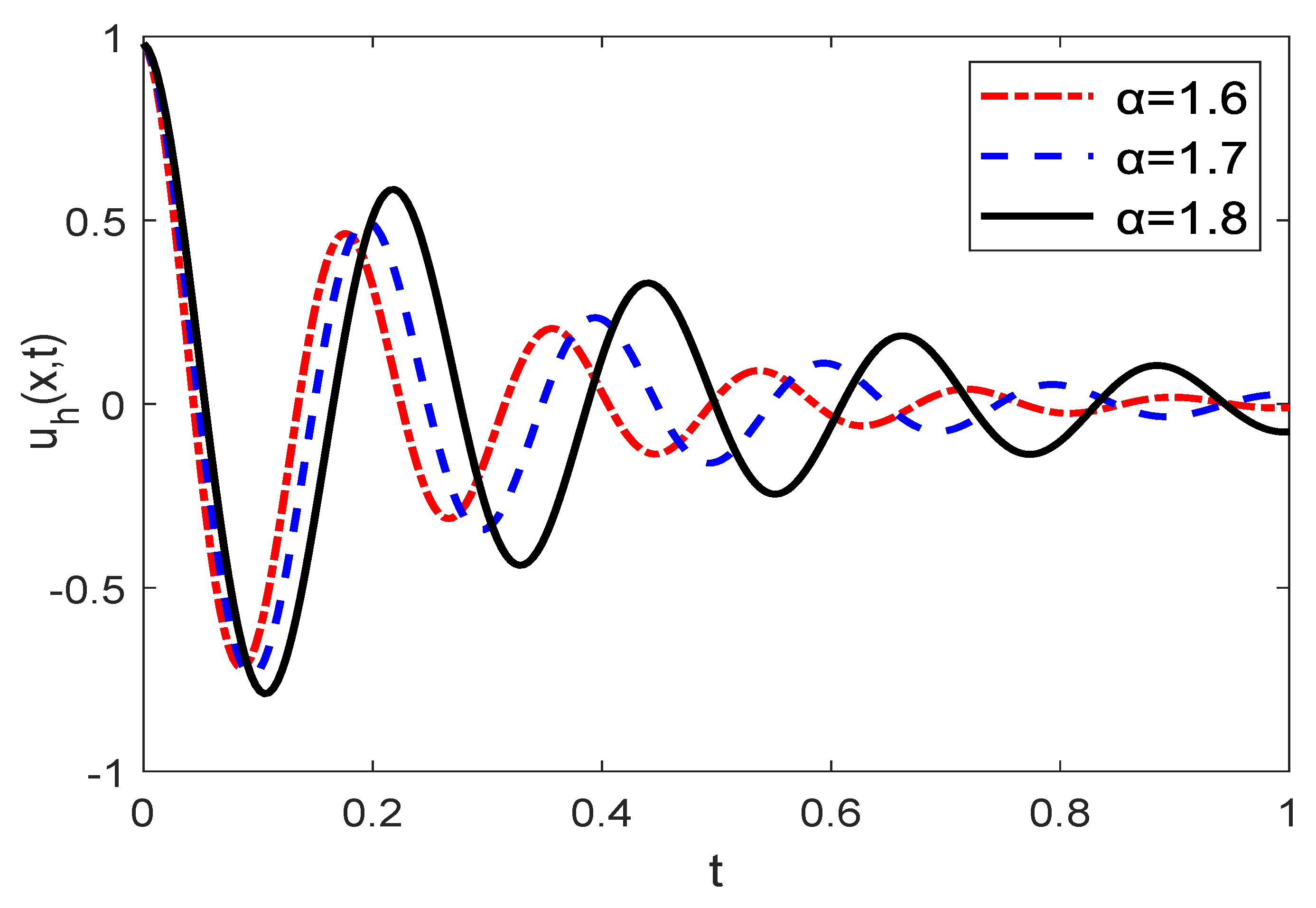
Next, we fixed , changed the value of and observed the vibration curve at the midpoint of the damping beam. It can be seen from Figure 8 that the attenuation rate of the beam vibration decreases with the increase in the order of the fractional derivative. In addition, it is generally shown that the peaks of these curves gradually increase and shift to the right as the order of the fractional derivatives increases.
7. Conclusions and Suggestions
In this paper, a mixed finite volume element method is proposed to solve the fractal-order damped beam vibration equation. By introducing two auxiliary variables with practical significance, the original fourth-order problem is transformed into a second-order equation system. The stability and convergence of the scheme are analyzed. The numerical examples demonstrate the effectiveness of the proposed method, and it can be seen that the larger the damping coefficient and the smaller the order of the fractional derivative, the faster the attenuation frequency of the beam vibration.
Although there are some other methods which can be used to solve such problems, the MFVE method shows its advantages: (i) The feature of the finite volume element scheme is retained, so the local conservation of physical quantities can be preserved. (ii) Two physical quantities with practical significance can be solved at the same time; thus, the computing cost is reduced. (iii) Compared with the finite element method, the space smoothness requirement is lower.
In the future work, we can apply this method to other types of beam vibration equations, such as beam vibration equations with structural damping, non-uniform beam vibration equations, etc. At the same time, other methods can be used to discretize the time derivatives to improve the accuracy of the method.
Author Contributions
Conceptualization, Z.J., A.Z. and Z.Y.; Writing—original draft, T.W.; Writing—review & editing, T.W. All authors have read and agreed to the published version of the manuscript.
Funding
This work is supported in part by the National Natural Science Foundation of China (contract grant number: 12171287, 11501335) and the Natural Science Foundation of Shandong Province (contract grant number: ZR2021MA063). The authors thank the reviewers for their helpful and valuable suggestions and comments on this paper.
Institutional Review Board Statement
Not applicable.
Informed Consent Statement
Not applicable.
Data Availability Statement
Not applicable.
Conflicts of Interest
The authors declare no conflict of interest regarding the publication of this paper.
References
- Nigmatullin, R.R. The realization of the generalized transfer equation in a medium with fractal geometry. Phys. Status Solidi (b) 1986, 133, 425–430. [Google Scholar] [CrossRef]
- Nikan, O.; Avazzadeh, Z.; Tenreiro Machado, J. Numerical approach for modeling fractional heat conduction in porous medium with the generalized Cattaneo model. Appl. Math. Model. 2021, 100, 107–124. [Google Scholar] [CrossRef]
- SHAN, L.; TONG, D.; XUE, L. Unsteady Flow of Non-Newtonian Visco-Elastic Fluid in Dual-Porosity Media with The Fractional Derivative. J. Hydrodyn. Ser. B 2009, 21, 705–713. [Google Scholar] [CrossRef]
- Luchko, Y.; Punzi, A. Modeling anomalous heat transport in geothermal reservoirs via fractional diffusion equations. GEM—Int. J. Geomath. 2010, 1, 257–276. [Google Scholar] [CrossRef]
- Wang, W.; Xia, X.G.; Zhang, S.; He, C.; Chen, L. Vector total fractional-order variation and its applications for color image denoising and decomposition. Appl. Math. Model. 2019, 72, 155–175. [Google Scholar] [CrossRef]
- Carlson, G.E.; Halijak, C. Approximation of Fractional Capacitors by a Regular Newton Process. IEEE Trans. Circuit Theory 1964, 11, 210–213. [Google Scholar] [CrossRef]
- Tong, D.; Wang, R. Analysis of the flow of non-Newtonian visco-elastic fluids in fractal reservoir with the fractional derivative. Sci. China Phys. Mech. Astron. 2004, 47, 424–441. [Google Scholar] [CrossRef]
- Sugimoto, N. Burgers equation with a fractional derivative; hereditary effects on nonlinear acoustic waves. J. Fluid Mech. 1991, 225, 631–653. [Google Scholar] [CrossRef]
- Gemant, A. A Method of Analyzing Experimental Results Obtained from Elasto-viscous Bodies. Physics 1936, 7, 311–317. [Google Scholar] [CrossRef]
- Demir, D.; Bildik, N.; SINIR, B. Application of fractional calculus in the dynamics of beams. Bound. Value Probl. 2012, 2012. [Google Scholar] [CrossRef] [Green Version]
- Demir, D.; Bildik, N.; SINIR, B. Linear dynamical analysis of fractionally damped beams and rods. J. Eng. Math. 2014, 85, 131–147. [Google Scholar] [CrossRef]
- Parmoon, R.; Rashidinia, J.; Parsa, A.; Haddadpour, H.; Salehi, R. Application of radial basis functions and sinc method for solving the forced vibration of fractional viscoelastic beam. J. Mech. Sci. Technol. 2016, 30, 3001–3008. [Google Scholar] [CrossRef]
- Cajic, M.; Karlicic, D.; Lazarevic, M. Damped vibration of a nonlocal nanobeam resting on viscoelastic foundation: Fractional derivative model with two retardation times and fractional parameters. Meccanica 2016, 52, 363–382. [Google Scholar] [CrossRef]
- Liu, D.; Xu, W.; Xu, Y. Stochastic response of an axially moving viscoelastic beam with fractional order constitutive relation and random excitations. Acta Mech. Sin. 2013, 29, 443–451. [Google Scholar] [CrossRef]
- Rossikhin, Y.; Shitikova, M. Application of fractional derivatives to the analysis of damped vibrations of viscoelastic single mass system. Acta Mech. 1997, 120, 109–125. [Google Scholar] [CrossRef]
- Faraji Oskouie, M.; Ansari, R.; Sadeghi, F. Nonlinear vibration analysis of fractional viscoelastic Euler-Bernoulli nanobeams based on the surface stress theory. Acta Mech. Solida Sin. 2017, 30, 416–424. [Google Scholar] [CrossRef]
- Yang, T.; Fang, B. Stability in parametric resonance of an axially moving beam constituted by fractional order material. Arch. Appl. Mech. 2012, 82, 1763–1770. [Google Scholar] [CrossRef]
- Cao, D.; Gao, Y.; Wang, J.; Yao, M.; Zhang, W. Analytical analysis of free vibration of non-uniform and non-homogenous beams: Asymptotic perturbation approach. Appl. Math. Model. 2019, 65, 526–534. [Google Scholar] [CrossRef]
- Liang, Z.; Tang, X. Analytical solution of fractionally damped beam by Adomian decomposition method. Appl. Math. Mech. (Engl. Ed.) 2007, 28, 219–228. [Google Scholar] [CrossRef]
- Patnaik, S.; Sidhardh, S.; Semperlotti, F. A Ritz-based finite element method for a fractional-order boundary value problem of nonlocal elasticity. Int. J. Solids Struct. 2020, 202, 398–417. [Google Scholar] [CrossRef]
- Stempin, P.; Sumelka, W. Formulation and experimental validation of space-fractional Timoshenko beam model with functionally graded materials effects. Comput. Mech. 2021, 68, 697–708. [Google Scholar] [CrossRef]
- Podlubny, I. Fractional Differential Equations. In Mathematics in Science and Engineering; Academic Press: Cambridge, MA, USA, 1999. [Google Scholar]
- Guo, B.; Pu, X.; Huang, F. Fractional Partial Differential Equations and Their Numerical Solutions; World Scientific: Singapore, 2015. [Google Scholar] [CrossRef]
- Gao, G.; Sun, Z.; Zhang, H. A new fractional numerical differentiation formula to approximate the Caputo fractional derivative and its applications. J. Comput. Phys. 2014, 259, 33–50. [Google Scholar] [CrossRef]
- Li, L.; Jiang, Z.; Yin, Z. Compact finite-difference method for 2D time-fractional convection–diffusion equation of groundwater pollution problems. Comput. Appl. Math. 2020, 39. [Google Scholar] [CrossRef]
- Jin, B.; Lazarov, R.; Zhou, Z. Error Estimates for a Semidiscrete Finite Element Method for Fractional Order Parabolic Equations. SIAM J. Numer. Anal. 2012, 51, 142. [Google Scholar] [CrossRef]
- Liu, Y.; Du, Y.; Li, H.; Wang, J. An H1 Galerkin mixed finite element method for time fractional reaction–diffusion equation. J. Appl. Math. Comput. 2014, 47, 103–117. [Google Scholar] [CrossRef]
- Su, B.; Jiang, Z. High-order compact finite volume scheme for the 2D multi-term time fractional sub-diffusion equation. Adv. Differ. Equ. 2020, 2020, 689. [Google Scholar] [CrossRef]
- Youssri, Y.H. Orthonormal Ultraspherical Operational Matrix Algorithm for fractal–fractional Riccati Equation with Generalized Caputo Derivative. Fractal Fract. 2021, 5, 100. [Google Scholar] [CrossRef]
- Youssri, Y. Two Fibonacci operational matrix pseudo-spectral schemes for nonlinear fractional Klein-Gordon equation. Int. J. Mod. Phys. C 2022, 33, 2250049. [Google Scholar] [CrossRef]
- Sabir, Z.; Munawar, M.; Abdelkawy, M.A.; Raja, M.A.Z.; Unlu, C.; Jeelani, M.B.; Alnahdi, A.S. Numerical Investigations of the Fractional-Order Mathematical Model Underlying Immune-Chemotherapeutic Treatment for Breast Cancer Using the Neural Networks. Fractal Fract. 2022, 6, 184. [Google Scholar] [CrossRef]
- Russell, T. Rigorous Block-Centered Discretizations on Irregular Grids: Improved Simulation of Complex Reservior Systems; Project Report; Technical Report No. 3; Resevoir Simulation Research Corporation: Tulsa, OK, USA, 1995. [Google Scholar]
- Sun, Z.; Wu, X. A fully discrete scheme for a diffusion-wave system. Appl. Numer. Math. 2006, 56, 193–209. [Google Scholar] [CrossRef]
- Li, R.; Chen, Z.; Wu, W. Generalized Difference Methods for Differential Equations (Numerical Analysis of Finite Volume Methods); CRC Press: Boca Raton, FL, USA, 2000. [Google Scholar]
- Wang, T. A mixed finite volume element method based on rectangular mesh for biharmonic equations. J. Comput. Appl. Math. 2004, 172, 117–130. [Google Scholar] [CrossRef]
- Fang, Z.; Li, H. Numerical solutions to regularized long wave equation based on mixed covolume method. Appl. Math. Mech. 2013, 34, 907–920. [Google Scholar] [CrossRef]
- Ren, J.; Xiaonian, L.; Mao, S.; Zhang, J. Superconvergence of Finite Element Approximations for the Fractional Diffusion-Wave Equation. J. Sci. Comput. 2017, 72, 917–935. [Google Scholar] [CrossRef]
Figure 1.
Graph of the displacement at when .

Figure 2.
Graph of the bending moment at when .

Figure 3.
Contour plot of when .

Figure 4.
Contour plot of when .
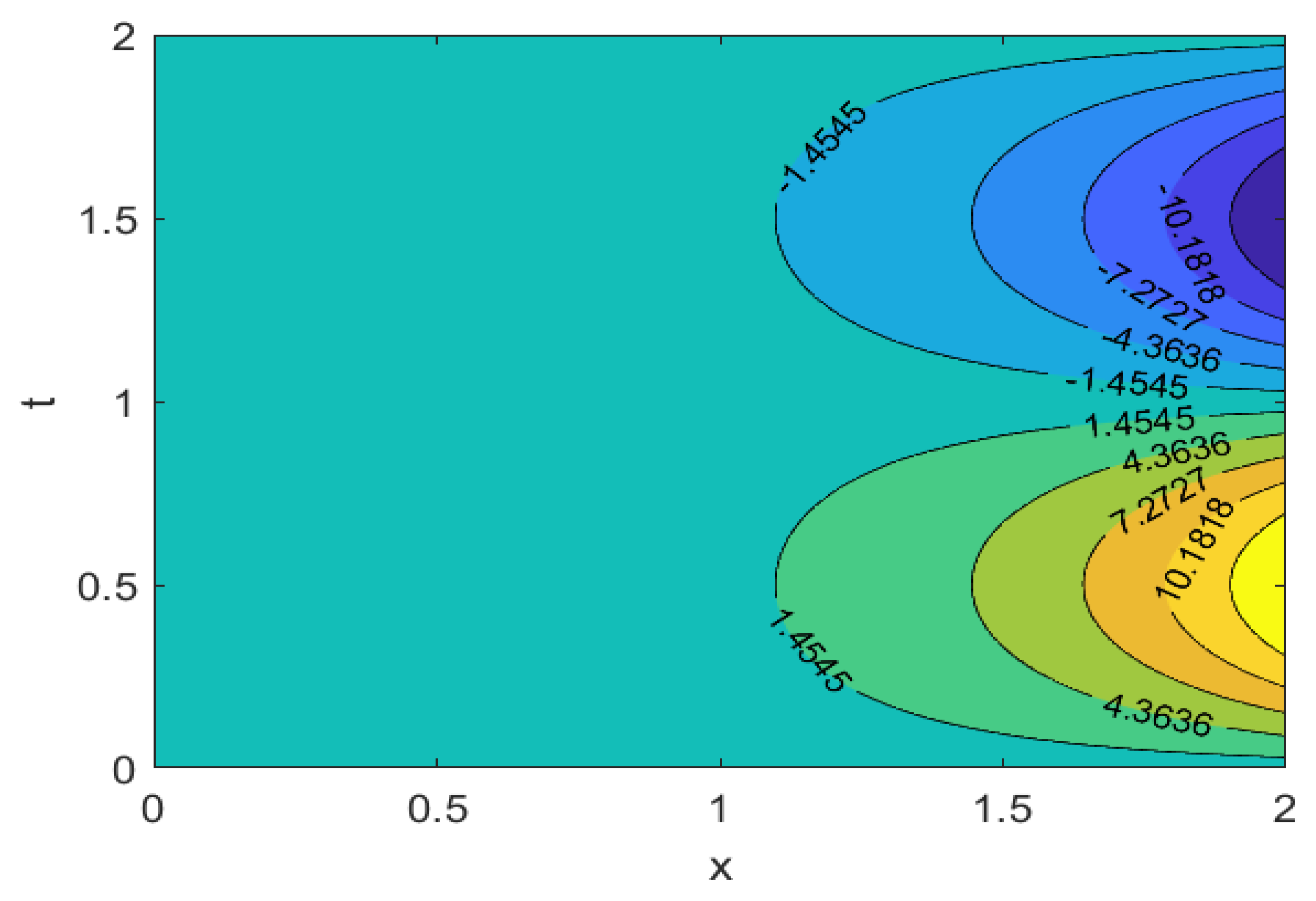
Figure 5.
Contour plot of for .

Figure 6.
Contour plot of when .
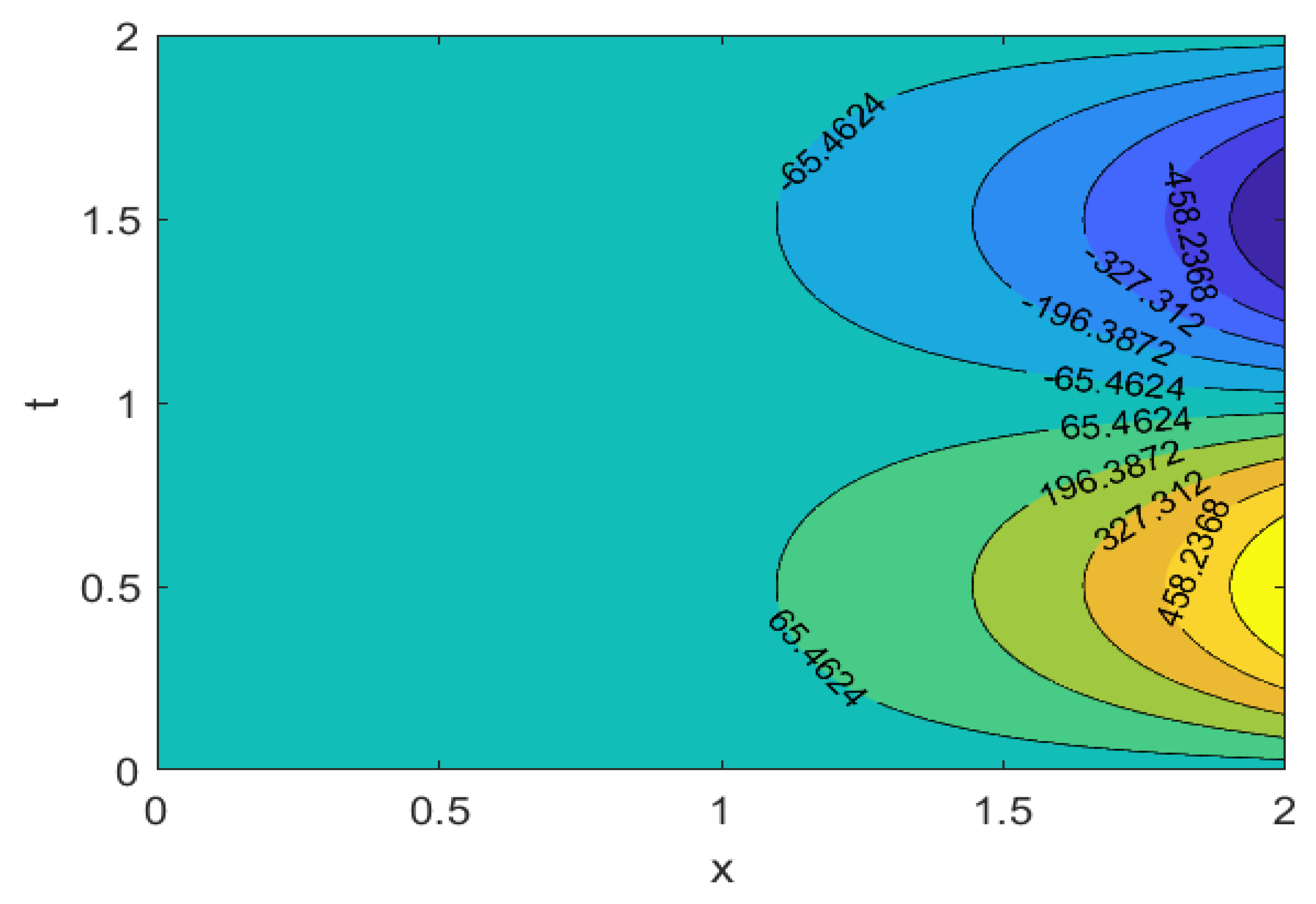
Figure 7.
Graph of at the midpoint over time for different values of .
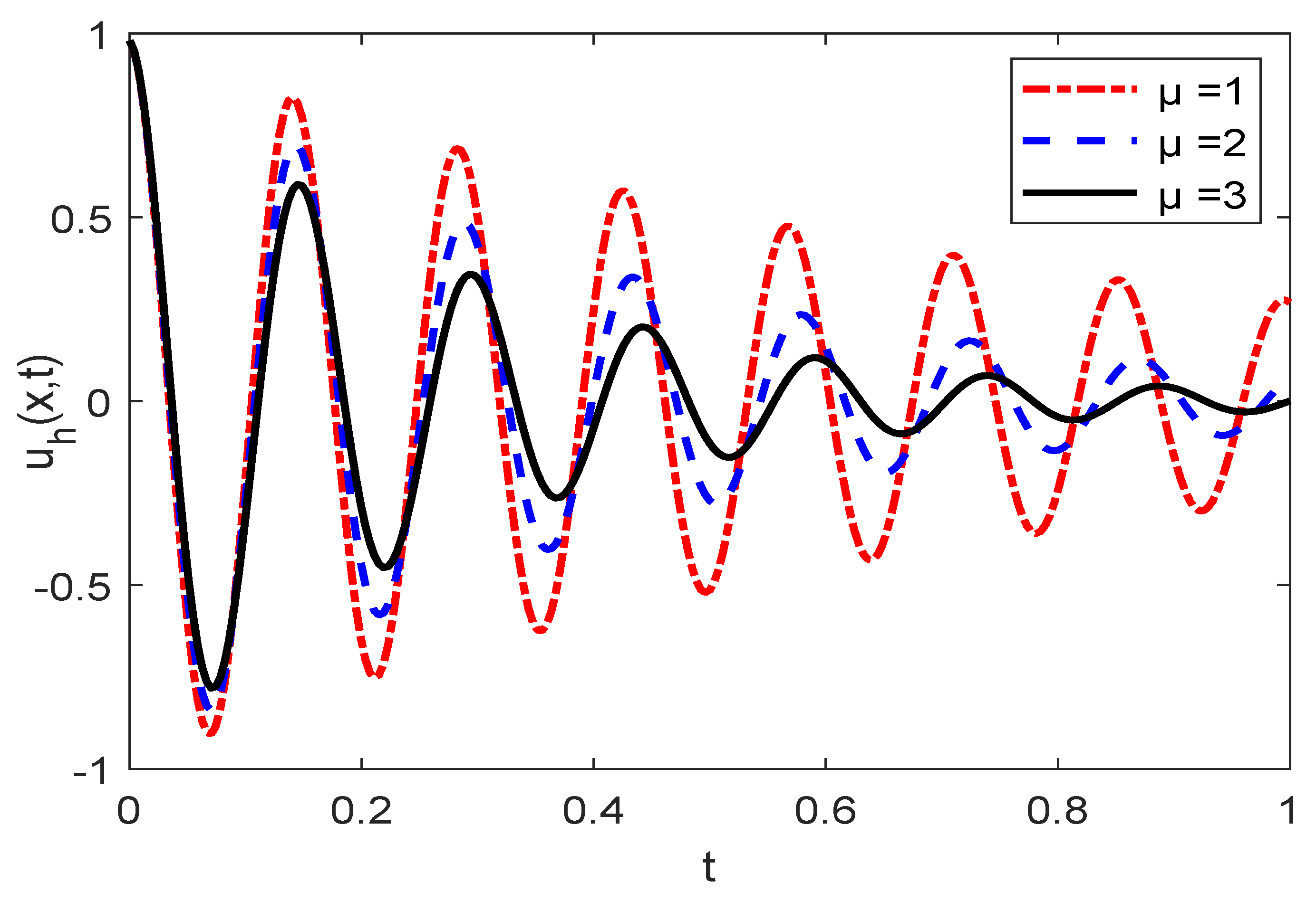
Figure 8.
Graph of at the midpoint over time for different values of .

Table 1.
-norm errors and temporal convergence order of MFVE method.
| Order | Order | Order | |||||
|---|---|---|---|---|---|---|---|
| 1/10 | 3.0223 | − | 4.0686 | − | 6.3215 | − | |
| 1/20 | 1.4641 | 1.046 | 2.0832 | 0.965 | 3.1727 | 0.995 | |
| 1/40 | 7.1948 | 1.025 | 1.0506 | 0.988 | 1.5877 | 0.999 | |
| 1/80 | 3.5650 | 1.013 | 5.2749 | 0.994 | 7.9404 | 1.000 | |
| 1/10 | 3.0233 | − | 4.0756 | − | 6.3245 | − | |
| 1/20 | 1.4641 | 1.046 | 2.0820 | 0.979 | 3.1726 | 0.995 | |
| 1/40 | 7.1945 | 1.025 | 1.0505 | 0.991 | 1.5877 | 0.999 | |
| 1/80 | 3.5648 | 1.013 | 5.2763 | 0.996 | 7.9393 | 1.000 |
Table 2.
-harf-norm errors and temporal convergence order of MFVE method.
| Order | Order | Order | |||||
|---|---|---|---|---|---|---|---|
| 1/10 | 9.4947 | − | 1.2782 | − | 1.9859×10 | − | |
| 1/20 | 4.5997 | 1.046 | 6.5446 | 0.966 | 9.9673 | 0.995 | |
| 1/40 | 2.2603 | 1.025 | 3.3004 | 0.988 | 4.9881 | 0.999 | |
| 1/80 | 1.1200 | 1.013 | 1.6572 | 0.994 | 2.4946 | 1.000 | |
| 1/10 | 9.4979 | − | 1.2804 | − | 1.9869×10 | − | |
| 1/20 | 4.5996 | 1.046 | 6.5407 | 0.969 | 9.9672 | 0.995 | |
| 1/40 | 2.2602 | 1.025 | 3.3001 | 0.987 | 4.9878 | 0.999 | |
| 1/80 | 1.1200 | 1.013 | 1.6576 | 0.993 | 2.4942 | 1.000 |
Table 3.
-norm errors and spatial convergence order of MFVE method.
| h | Order | Order | Order | ||||
|---|---|---|---|---|---|---|---|
| 1/8 | 4.4899 | − | 6.6632 | − | 1.2098 | − | |
| 1/16 | 1.1115 | 2.014 | 1.6676 | 1.999 | 3.0108 | 2.007 | |
| 1/32 | 2.7719 | 2.004 | 4.1700 | 2.000 | 7.5184 | 2.002 | |
| 1/64 | 6.9254 | 2.001 | 1.0426 | 2.000 | 1.8790 | 2.000 | |
| 1/8 | 4.4911 | − | 6.6675 | − | 1.2104 | − | |
| 1/16 | 1.1117 | 2.014 | 1.6683 | 1.999 | 3.0118 | 2.007 | |
| 1/32 | 2.7722 | 2.004 | 4.1717 | 2.000 | 7.5200 | 2.002 | |
| 1/64 | 6.9260 | 2.001 | 1.0430 | 2.000 | 1.8793 | 2.001 |
Table 4.
-harf-norm errors and spatial convergence order of MFVE method.
| h | Order | Order | Order | ||||
|---|---|---|---|---|---|---|---|
| 1/8 | 1.4015 | − | 2.0800 | − | 3.7764 | − | |
| 1/16 | 3.4863 | 2.007 | 5.2305 | 1.992 | 9.4436 | 2.000 | |
| 1/32 | 8.7046 | 2.002 | 1.3095 | 1.998 | 2.3610 | 2.000 | |
| 1/64 | 2.1755 | 2.001 | 3.2750 | 2.000 | 5.9026 | 2.000 | |
| 1/8 | 1.4019 | − | 2.0812 | − | 3.7781 | − | |
| 1/16 | 3.4869 | 2.007 | 5.2328 | 1.992 | 9.4465 | 2.000 | |
| 1/32 | 8.7057 | 2.002 | 1.3101 | 1.998 | 2.3615 | 2.000 | |
| 1/64 | 2.1756 | 2.001 | 3.2762 | 2.000 | 5.9035 | 2.000 |
Publisher’s Note: MDPI stays neutral with regard to jurisdictional claims in published maps and institutional affiliations. |
© 2022 by the authors. Licensee MDPI, Basel, Switzerland. This article is an open access article distributed under the terms and conditions of the Creative Commons Attribution (CC BY) license (https://creativecommons.org/licenses/by/4.0/).
Share and Cite
MDPI and ACS Style
Wang, T.; Jiang, Z.; Zhu, A.; Yin, Z. A Mixed Finite Volume Element Method for Time-Fractional Damping Beam Vibration Problem. Fractal Fract. 2022, 6, 523. https://doi.org/10.3390/fractalfract6090523
AMA Style
Wang T, Jiang Z, Zhu A, Yin Z. A Mixed Finite Volume Element Method for Time-Fractional Damping Beam Vibration Problem. Fractal and Fractional. 2022; 6(9):523. https://doi.org/10.3390/fractalfract6090523
Chicago/Turabian StyleWang, Tongxin, Ziwen Jiang, Ailing Zhu, and Zhe Yin. 2022. "A Mixed Finite Volume Element Method for Time-Fractional Damping Beam Vibration Problem" Fractal and Fractional 6, no. 9: 523. https://doi.org/10.3390/fractalfract6090523