
Adaptive Fuzzy Fault-Tolerant Control of Uncertain Fractional-Order Nonlinear Systems with Sensor and Actuator Faults


1
College of Science, Liaoning University of Technology, Jinzhou 121001, China
2
School of Mathematics and Statistics, Guangdong University of Foreign Studies, Guangzhou 510006, China
*
Author to whom correspondence should be addressed.
Fractal Fract. 2023, 7(12), 862; https://doi.org/10.3390/fractalfract7120862
Submission received: 14 October 2023
/
Revised: 27 November 2023
/
Accepted: 30 November 2023
/
Published: 4 December 2023
(This article belongs to the Special Issue Advances in Fractional-Order Multiagent Systems: Theory and Applications)
Abstract
:In this work, an adaptive fuzzy backstepping fault-tolerant control (FTC) issue is tackled for uncertain fractional-order (FO) nonlinear systems with sensor and actuator faults. A fuzzy logic system is exploited to manage unknown nonlinearity. In addition, a novel FO nonlinear filter-based dynamic surface control (DSC) method is constructed, effectively avoiding the inherent complexity explosion problem in the backstepping recursive process, and in the light of the construction of auxiliary functions, compensating the coupling term introduced by faults. On account of certain assumptions, the stability criterion of the FO Lyapunov function is applied to guarantee the stability of the closed-loop system. Finally, the simulation example verifies the validity of the presented control strategy.
1. Introduction
The fractional order system is an extension of the integer-order system in traditional control theory. It can describe non-rigid dynamic systems more accurately, and has been widely used in bioengineering, thermoelectric systems, electronic power systems, battery management systems and so on. In recent years, with the wide application of fractional-order systems, fractional-order control theory has been developed rapidly and made some progress. To go a step further, a vast array of fascinating results has been gained for controller design of fractional order systems [1,2,3,4]. However, the above works are only applied to fractional order systems in which the system mode is linear or the nonlinearities are known. Thus, these schemes cannot be applied to fractional-order systems with unknown nonlinearities. Generally speaking, due to changes in the internal or external environment of the system, nonlinear and uncertainty often exist simultaneously in the control research of nonlinear systems, which makes the control design and stability analysis of the FO nonlinear systems extremely difficult. Therefore, some scholars have studied the control design of fractional nonlinear systems and made some progress [5,6,7,8]. In [5], a fractional order fast terminal sliding mode control method is proposed under the assumption that the nonlinear function is bounded. In [6,7], state feedback control methods based on the indirect Lyapunov method and direct Lyapunov method are proposed for Lipschitz-type nonlinear systems and multi-agent nonlinear systems, respectively. Further, for linear parameterized fractional-order nonlinear systems, an adaptive control method based on fractional-order parameter updating law is presented in [8]. The control design method proposed in [5,6,7,8] requires that the nonlinear system must meet the matching condition, that is, the nonlinearity of the system must appear in the same equation as the controller, and the control scheme obtained is established under the theoretical framework of feedback linearization. In order to solve the control problem that the controlled object is a strict feedback nonlinear system (a nonlinear system that meets the non-matching conditions), with the help of backstepping control technology and based on direct Lyapunov function method, fractional adaptive backward step recursive state feedback and output feedback control methods are presented in [9,10], respectively. Based on the indirect Lyapunov function method, the authors in [11,12] proposed adaptive backstepping recurrent state feedback and output feedback control methods, respectively.
At present, although some research achievements have been made in the control problems of frit-order nonlinear systems, the above research methods all require that the model of the controlled object is known or the nonlinear function can be parameterized. Obviously, a great majority of the works of fractional-order adaptive control assume that uncertainties existing in the system can be linearly parameterized, which is unrealistic in practical control design. Therefore, it is a challenging task to solve the controller design problem for FO nonlinear systems with unknown nonlinear functions. To handle such an issue, since fuzzy logic systems or neural networks have good approximation and learning ability to unknown nonlinear dynamics, nonlinear intelligent control schemes based on fuzzy logic systems or neural networks are often developed, and are widely used in uncertain fractional-order nonlinear systems, and many fruitful research results are achieved [13,14,15,16,17,18]. The main representative achievements are as follows: in [13], a fuzzy adaptive backstepping recursive state feedback control scheme is proposed for the nonlinear system with uncertain fractional order strict feedback with single input and single output. In the design process, fuzzy logic system is used to model the unknown nonlinear system, and the parameters are updated online by designing the fractional order adaptive law. Based on finite-time sliding mode control theory, a fractional-order finite-time fuzzy adaptive state feedback sliding mode control method is proposed in [14,15] for single-input single-output uncertain fractional-order strict feedback nonlinear systems. For uncertain switching fractional-order nonlinear systems, based on the common Lyapunov function method, a fractional-order switching neural network adaptive state feedback control scheme is proposed in [16]. In [17,18], for uncertain fractional nonlinear multi-agent systems, the robust consistency tracking problem in general undirected topology and directed topology is studied by using neural network to model the controlled object. Although fractional nonlinear systems have made some achievements in the design of adaptive control and fuzzy/neural network control, the above achievements are all under the premise of normal operation of the system actuator or sensor. When actuator or sensor failure occurs in the system, the above method can not meet the dual requirements of control performance and stability analysis. If the fault can not be identified and compensated in time, the control accuracy is bound to decline, and even affect the normal operation of the system.
In practical engineering, there usually exists an inescapable fact that system components (e.g., actuators, sensors, etc.) may abruptly encounter an unexpected occurrence during the operating process, which impairs system performance, disrupts system stability, and even potentially triggers a fatal disaster [19,20]. To assure reliability and security, the area of exploring faults has drawn intensive concern. Regarding this, the FTC strategy was presented, aiming at handling various faults while ensuring system stability and performance, and recently fruitful developments have been reported on actuator faults [21,22,23,24,25,26,27]. Focusing on linear systems, several FTC approaches were designed to tackle partial loss of effectiveness and locked faults [21,22], further extended in distinct varieties to nonlinear cases [23,24,25,26,27]. Nevertheless, collating the aforementioned works, it is obvious that they only concentrate on the integer-order nonlinear case. Actually, compared to traditional integer-order case, FO nonlinear systems have broader prospects due to their unique characteristics, e.g., memory and inheritance, and have received the favor of numerous scholars. Certainly, the achievements on actuator faults in FO nonlinear systems will not be absent [28,29,30,31,32]. Through the sliding mode control technique, the FTC issue of triangular FO nonlinear systems with actuator faults was addressed [28], where the multiple control inputs are translated into the special mode in view of actuator fault characteristics, while the nonlinear dynamics considered in [28] must meet the matching condition. Further, the authors in [29] extend the previous results to control nonlinear systems with actuator faults that the non-matching condition is not satisfied. On the basis of adaptive control technique, actuator faults coefficients are effectively estimated in [30], where the fault compensation relies on the introduction of multiple parameter adaptive laws, which inevitably increases the complexity of the controller. To erase such a limitation, the Nussbaum gain technique is introduced in [31] to handle the lumped uncertainties of multiple faulty actuators and unknown control gains; however, the catch is that high-frequency oscillations may occur. It should be emphasized that the above control methods are only suitable for the limited number of faults in the actuator, and the fault mode remains unchanged. Aiming at this issue, a special auxiliary function is employed in [32] to compensate the effect of intermittent actuator faults. Unfortunately, this method relies too much on the ability of approximation technique, which may reduce the performance. Although the research on intelligent fault-tolerant control for uncertain fractional nonlinear systems has achieved some achievements, the works [28,29,30,31,32] are limited to the study of actuator fault compensation control, and the fault-tolerant control of fractional nonlinear systems with sensor faults is not reported. It is vital to be aware that the sensor is more prone to faults than the actuator, and the case sensor encounter unexpected occurrence may be even worse since misleading information from faulty sensors causes the entire system to be embroiled in risks. Note that in actuator faults compensation control design, the actuator’s output is dependent on the output of controller u, where u is available but is unknown. Meanwhile, in the sensor faults case, the measurement values depend on unknown system state variables . It is obvious that the previous actuator faults compensation schemes are invalid for sensor faults compensation control problem. Thus, it is still a tremendous challenge to develop a sensor FTC strategy, not to mention the case with both actuator and sensor faults.
Meanwhile, with the repeated differentiation of the virtual control function and the continuous increase of the system dimension in the control process, the computational load of the backstepping control design is obviously terrible. This phenomenon is known as computational expansion. For the sake of maintaining system stability and reducing the computational burden existed in traditional backstepping recursive methods, the inverse control design idea based on filter technology was presented for the first time in [33]. Similar ideas were also explored in [34,35]. However, the results obtained based on this technique in [33,34,35] only referred to the integer-order nonlinear case. Compared to the integer-order case, the parameters in FO case have more degrees of freedom, resulting in the inapplicability of Newton–Leibniz formula and the derivative rules in integer-order case, which hence makes it exceedingly thorny to employ integer-order control method directly to FO. In [36,37], authors drew on the aforementioned ideas to explore FO, and made momentous progresses via linear filter, while neglecting the compensation of the error boundary, which lead to the increase of the error boundary. In order to better compensate the boundary errors, which were caused by the introduction of the filter, the authors of [38,39] proposed the design idea of nonlinear filtering by introducing auxiliary functions, and, combined with the traditional backstepping control, they effectively avoided the computational expansion and the impact of the boundary error. But the common feature of these works is that the actuators and sensors in the FO systems studied are under normal conditions. In the process of research, we find that when both actuators and sensors fail, it would bring about the emergence of coupling terms. Unfortunately, these existing nonlinear filtering-based strategies cannot deal with the coupling terms caused by the coexistence of actuator and sensor faults.
Enlightened by the above motivations, we focus on the adaptive fuzzy FTC problem for FO nonlinear systems with both actuator and sensor faults. The main contributions of this paper are divided into two points:
- (1)
- This paper addresses the FTC issue of FO nonlinear systems with simultaneous actuator faults and sensor faults. It should be mentioned that unlike this paper, the authors in [28,29,30,31,32] considered the adaptive fault-tolerant control issue for fractional-order nonlinear systems with actuator faults. However, in the actual control system, the sensor is more prone to failure than the actuator, and the performance of the system is also heavily dependent on the output signal of the sensor, so even if the sensor undergoes a small fault, the feedback control and stability of the closed-loop system will be greatly affected. It is obvious that the previous actuator faults compensation schemes are invalid for sensor faults compensation control problem, not to mention the case with both actuator and sensor faults. This makes the research of this work more difficult and challenging.
- (2)
- A nonlinear filtering-based DSC strategy is established by introducing auxiliary functions, which not only effectively solves the issue of computational burden existing in traditional FO nonlinear strict feedback systems, but also improves the control performance in contrast to the traditional linear filters-based DSC results [36,37]. Different from nonlinear filtering results [38,39], this paper compensates the effects of lumped uncertainties caused by actuator faults and sensor faults by designing a quadratic Lyapunov function which includes the lower bound of actuator and sensor faults coefficients.
- (3)
- The proposed fault compensation mechanism can erase the limitation condition that the unknown functions dependent on state variable must satisfy the monotonically increasing property, by use of the characteristics of fuzzy basis functions.
The paper is organized as follows. The preliminaries and problem formulation are presented in Section 2. In Section 3, nonlinear filter-based adaptive controller design and stability analysis are addressed. Effectiveness of the proposed scheme has been demonstrated via simulation study in Section 4. The conclusion is drawn in Section 5.
Notation.
In this paper, some specific notations are employed. C represents a complex set; N is a set of natural numbers; is the absolute value of real number; denotes the Euclidean norm of a vector or the corresponding induced norm of a matrix; denotes i-dimensional Euclidean space.
2. Preliminaries and Problem Formulation
2.1. Preliminaries
To facilitate the subsequent strategy, several preliminaries are presented.
Definition 1
([40]). A continuous function , is said to belong to class-K if it is strictly increasing and .
Definition 2
([41]). Let be a class-K function, then its FO integral satisfies
with , being the fractional–integral of order ω subject to initial time , the Gamma function is denoted as , where . A key property for Gamma function is that , , .
Definition 3
Lemma 1
Lemma 2
([41]). Denote satisfying , and satisfying , then for any integer ,
with and . Here, represents the Mittag–Leffler function defined as:
Lemma 3
([41]). Consider the real numbers ν, , ω and ι defined in Lemma 2. Then, the following inequality holds
where .
Lemma 4
([43]). Consider FO nonlinear system with being Lipschitz continuous, whose equilibrium point is . For class-K functions (), and function , if
hold, asymptotical stability of the system is achieved.
Lemma 5
([44]). Denote be a continous function on a compact set . Then, , a FLS satisfies
where denotes the fuzzy basis function satisfying the fact that , while denotes the optimal weight, ı being the maximum rule number, and κ being regarded as a bounded fuzzy approximation error.
2.2. Problem Formulation
Consider a class of FO nonlinear systems with sensor and actuator faults in following form:
with () being the system states, and being the output of actuator and system, , and smooth functions () being unknown.
Remark 1.
System (9) concerned in this article is more universal than results [28,29,30,31,32], since in this work each subsystem involves a sensor fault and the last subsystem contains an actuator and sensor fault. The coupling term induced by sensor fault is quite distinct from the traditional coupling term, which determines that this work is more challenging. In the sequel, we will present a novel FO nonlinear filter to tackle it.
This work considers potential faults that occurred on actuator and sensors simultaneously, whose definitions are presented as follows
Definition 4
([32,45]). The actuator fault is
with , being unknown but bounded, denotes actuator fault occurrence time.
The s-th sensor fault is
with , , denotes bias faults that is unknown but bounded, denote sensor faults occurrence time.
The fault and () can be divided into 4 cases, as described in Table 1, where ().
The block diagram of the fractional-order nonlinear systems with actuator and sensor faults is provided in Figure 1.
Remark 2.
From Figure 1, it is obvious that the function of the sensor is to transmit the signal from the system to the controller, while the transmitted signal will be biased due to the existence of sensor failure. However, sensors are detection devices that can feel the information being measured, thus the measurement values after sensor faults are measurable. In fact, since that the fault coefficients and are unknown, the states become unknown, which makes control design difficult and challenging to some extent.
Control Objective: Construct a FO nonlinear filter-based adaptive controller for system (9), to guarantee: (1) all the closed-loop signals are bounded; (2) the system output y is forced to track the reference tracjectory .
To this end, some assumptions and lemmas are needed.
Assumption 1
([32]). and are limited by unknown constants and , i.e., and .
Lemma 6
3. Nonlinear Filter-Based Adaptive Controller Design and Stability Analysis
3.1. Novel Nonlinear Filter Design
To avoid the issue of explosion of complexity, a valid nonlinear filter is constructed
with
where , , filter is utilized in place of the intermediate controller , while represents the ℓ-th boundary layer error. and are emplyed to estimate and with , () and being the unknown upper bounds of , and , respectively.
Remark 3.
In contrast to the classical strategy utilizing linear filter [36], the merit of presented method lies in that the constructed nonlinear filter is reflected in the introduction of and , in which the former is employed to counterbalance the upper bound of the derivative of the virtual control law, while the latter is employed to expunge the coupling effect emerged from the actuator and sensor faults.
3.2. Adaptive Controller Design
In this work, the adaptive backstepping FTC scheme will be proposed in accordance with the changes of coordinates:
with being a measurement value, being an error surface, being obtained according to an FO filter on and being the FO filter output error designed in the sequel.
For the sake of simplicity, we will omit state dependence.
Owing to the unknown property of function , fuzzy logic system is utilized to model as
where with being the ideal weight, and being bounded by .
Define the Lyapunov function candidate
where and are design constants, , and , and and denote the estimations of and , respectively, with .
In the light of Young’s Inequality, one can compute
Define with , then, on the basis of Proposition 1 in [50], it yields
where is a constant. In accordance with (15), one can deduce
where will be given later. Using (21)–(24), becomes
The virtual control law can be given as
with being defined as
where is a constant. In terms of Lemma 6, one can calculate
Then (25) satisfies
with . Construct the adaptive law and as
where and are design constants. Substituting (30) and (31) into (29) produces
Similarly, due to the unknown property of function , fuzzy logic system is utilized to model as
with being the ideal weight, and being bounded by .
Define the Lyapunov function candidate
where , , and are design constants, , and , and and denote the estimations of and , respectively, with .
In a similar way to the first step, one can obtain
Denote with , then, it is easy to obtain
where is a constant. Thus, one can describe
with being given later. Then, some transformations are established as
The virtual control law is given as
with being defined as
where is a constant. According to Lemma 6, one can calculate
Then, (46) satisfies
where .
Construct the adaptive laws , , and as
with , , and being design constants. Invoking (48)–(51) produces
Define the Lyapunov function
where , , and are design constants, , and . Note that and are the estimates of and , respectively, where , with .
The actual controller is given as
with being defined as
where is a constant, (), .
3.3. Stability Analysis
The presented control scheme achieves the following result.
Theorem 1.
Consider an uncertain FO nonlinear system with actuator and sensor faults (9) subject to Assumptions 1–3. Through the virtual control laws (26) and (44), the actual control law (55) and the adaptive laws (30) and (31), (48)–(51) and (57)–(60), it is ensured that all the closed-loop signals are bounded, and the output y follows the desired signal well.
Proof.
Denote , hence a constant exists such that , on compact set . □
Denote . Then, there must exist a parameter satisfying
Taking Laplace transform on (67) becomes
which indicates
where ∗ denotes the convolution operator. Using Lemma 2 induces
Thus, the last term in (69), i.e., is negative.
Since , and , in the light of Lemma 3,
Then, one can know via Assumption 3 that
Consequently, one can find a time instant , for and , it is guaranteed that
Denote integer , using Lemma 1 gives
which induces
On the basis of the definition of infinitesimal amount, it is clear that , , with and being a time instant. Hence, (75) is rearranged as
where . Subsequently, one can conclude
Thus, the boundedness of all the closed-loop signals is guaranteed, and the tracking error approaches a small neighborhood of the original , for all .
4. Simulation Study
A Chua–Hartley system [51] is considered to demonstrate the reliability of the presented FTC approach:
where . When , system (78) shows rich dynamical behavior, which is depicted in Figure 2.
The sensor and actuator faults are selected as follows:
with , , , , , , , , , .
Three fuzzy logic systems are employed to estimate the unknown nonlinearities existed in system (78). The fuzzy membership functions are chosen as: , , .
In order to explore the influence of controller gains on system tracking error, two cases are considered:
CASE 1: Controller gains are chosen as: .
In this case, the design parameters in a fault-tolerant controller, the adaptive laws parameters and fractional-order nonlinear filters are selected as: , , , , , , , , , , , , , , , , ().
The initial conditions are: , , , , , , , , , and , the others are zeros. The desired trajectory is chosen as .
The simulation results are shown in Figure 3, Figure 4, Figure 5, Figure 6 and Figure 7, the trajectories of y, and are showed in Figure 3; the trajectories of states () are depicted in Figure 4; the trajectories of and () are showed in Figure 5; the trajectories of and () are depicted in Figure 6; the control input is shown in Figure 7.
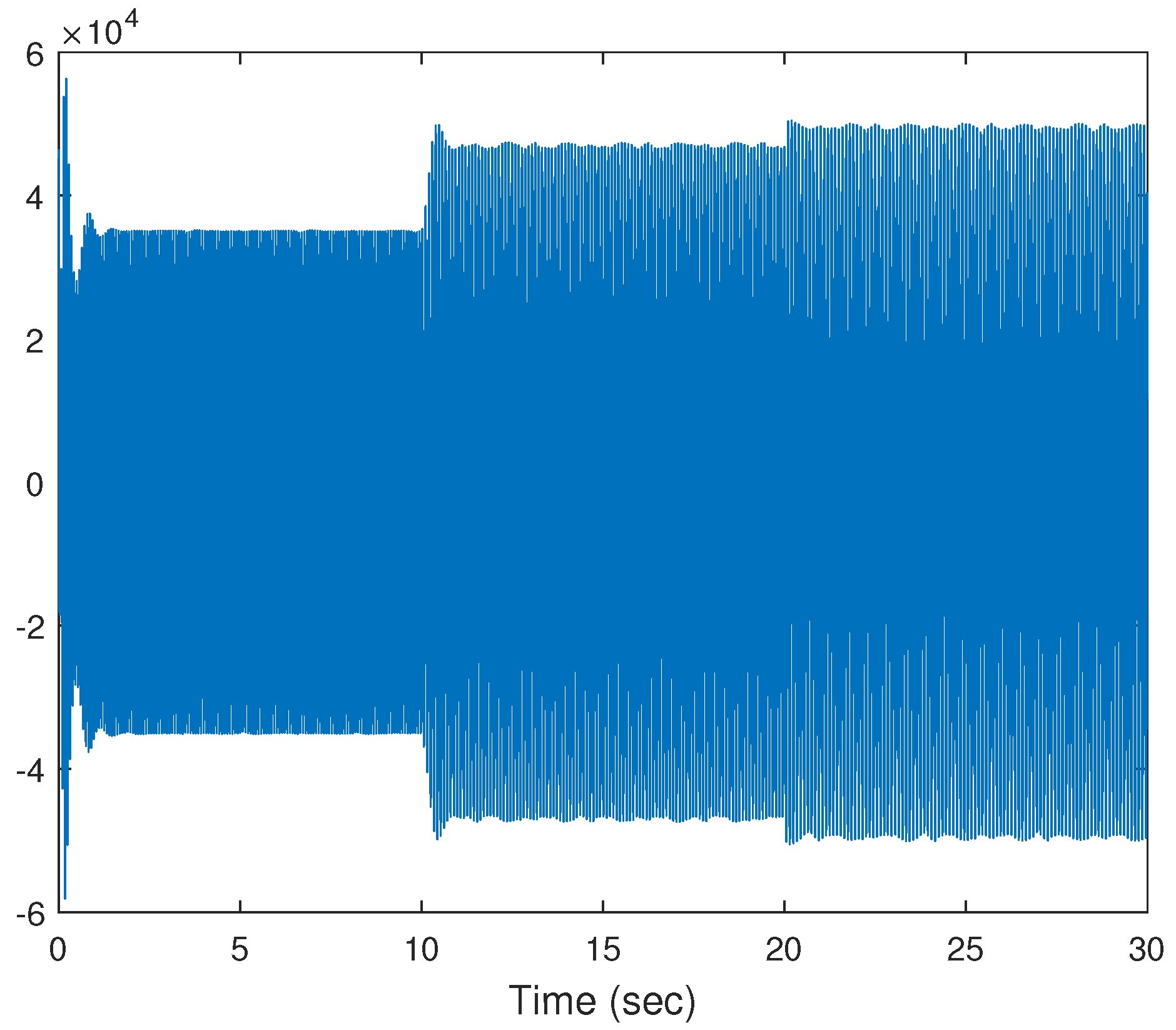
CASE 2: Controller gains are chosen as: .
In this case, the design parameters in the fault-tolerant controller, the adaptive laws parameters and fractional-order nonlinear filters and initial conditions are same as CASE 1.
The contrastive simulation results for the trajectories of y, and the control input are depicted in Figure 8 and Figure 9, respectively.
From the aforementioned simulation results, it is obvious that the following conclusions are proved.
- (i)
- (ii)
In summary, if the controller gain is increased, the tracking performance will be better. On the contrary, if you reduce controller gain, tracking performance deteriorates. Therefore, in practical applications, it is necessary to trade-off the transient performance and control action by selecting the design parameters suitably.
To better show the advantages of this paper in dealing with simultaneous actuator and sensor faults, we apply the existing adaptive control scheme for nonlinear systems with actuator and sensor faults using the fuzzy approximation criterion [45] to the Chua-Hartley system (78). Under the similar design parameters and initial conditions of CASE 1, the simulations results are shown in Figure 10 and Figure 11. It is clear that under the premise of similar tracking effect, the control input of our proposed control method is much smaller than the one in [45].
Remark 4.
By comparing Figure 7 and Figure 11, it is easy to see that the results in [45] rely too much on the ability of the approximation technique, which has to improve the tracking performance by only increasing the control gains constantly. In comparison to [45], the control design method proposed in this paper has higher design freedom, and shows better robustness and transient performance.
5. Conclusions
This work has addressed the adaptive fuzzy FTC issue for uncertain FO nonlinear systems with sensor and actuator faults. The fuzzy logic syatem has been exploited to manage unknown nonlinearity. On account of the constructed FO nonlinear filters, a DSC strategy has been developed. In line with the stability criterion of FO Lyapunov function, the system stability has been achieved. Exploring state constraints while maintaining a similar philosophy of the presented scheme is an interesting challenge for future study.
Author Contributions
Conceptualization, Z.M.; Methodology, K.S., Z.M. and P.G.; Software, G.D.; Validation, G.D.; Formal analysis, G.D. and P.G.; Investigation, K.S.; Writing—original draft, K.S.; Writing—review and editing, Z.M.; Visualization, P.G.; Supervision, Z.M.; Funding acquisition, Z.M. All authors have read and agreed to the published version of the manuscript.
Funding
This work is supported in part by the National Natural Science Foundation of China, under Grant 62203199 and 62003142, in part by the General Project of Natural Science Foundation of Liaoning Province, under Grant 2023-MS-299 and 2023-BS-194, and in part by the General Project of Liaoning Provincial Department of Education, under Grant LJKMZ20220974 and LJKQZ20222435.
Data Availability Statement
All data were presented in the main text.
Conflicts of Interest
The authors declare no conflict of interest.
References
- Lu, J.G.; Chen, G. Robust stability and stabilization of fractional-order interval systems: An LMI approach. IEEE Trans. Autom. Control. 2009, 54, 1294–1299. [Google Scholar]
- Lan, Y.H.; Zhou, Y. LMI-based robust control of fractional-order uncertain linear systems. Comput. Math. Appl. 2011, 62, 1460–1471. [Google Scholar] [CrossRef]
- Wei, Y.H.; Peter, W.T.; Yao, Z.; Wang, Y. The output feedback control synthesis for a class of singular fractional order systems. ISA Trans. 2017, 69, 1–9. [Google Scholar] [CrossRef] [PubMed]
- Djennoune, S.; Bettayeb, M. Optimal synergetic control for fractional-order systems. Automatica 2013, 49, 2243–2249. [Google Scholar] [CrossRef]
- Wang, B.; Ding, J.L.; Wu, F.J.; Zhu, D.L. Robust finite-time control of fractional-order nonlinear systems via frequency distributed model. Nonlinear Dyn. 2016, 85, 2133–2142. [Google Scholar] [CrossRef]
- Lan, Y.H.; Zhou, Y. Non-fragile observer-based robust control for a class of fractional-order nonlinear systems. Syst. Control. Lett. 2013, 62, 1143–1150. [Google Scholar] [CrossRef]
- Gong, P. Distributed tracking of heterogeneous nonlinear fractional-order multi-agent systems with an unknown leader. J. Frankl. Inst. 2017, 354, 2226–2244. [Google Scholar] [CrossRef]
- Chen, K.; Tang, R.N.; Li, C.; Wei, T.N. Robust adaptive fractional-order observer for a class of fractional-order nonlinear systems with unknown parameters. Nonlinear Dyn. 2018, 94, 415–427. [Google Scholar] [CrossRef]
- Ding, D.S.; Qi, D.L.; Wang, Q. Non-linear Mittag–Leffler stabilisation of commensurate fractional-order non-linear systems. IET Control. Theory Appl. 2015, 9, 681–690. [Google Scholar] [CrossRef]
- Hua, C.C.; Zhang, T.; Li, Y.F.; Guan, X.P. Robust output feedback control for fractional order nonlinear systems with time-varying delays. IEEE/CAA J. Autom. Sin. 2016, 3, 477–482. [Google Scholar]
- Wei, Y.H.; Chen, Y.Q.; Liang, S.; Wang, Y. A novel algorithm on adaptive backstepping control of fractional order systems. Neurocomputing 2015, 165, 395–402. [Google Scholar] [CrossRef]
- Wei, Y.H.; Tse, P.W.; Yao, Z.; Wang, Y. Adaptive backstepping output feedback control for a class of nonlinear fractional order systems. Nonlinear Dyn. 2016, 86, 1047–1056. [Google Scholar] [CrossRef]
- Liu, H.; Pan, Y.; Li, S.; Chen, Y. Adaptive fuzzy backstepping control of fractional-order nonlinear systems. IEEE Trans. Syst. Man Cybern. Syst. 2017, 47, 2209–2217. [Google Scholar] [CrossRef]
- Song, S.; Zhang, B.; Xia, J.; Zhang, Z. Adaptive backstepping hybrid fuzzy sliding mode control for uncertain fractional-order nonlinear systems based on finite-time scheme. IEEE Trans. Syst. Man Cybern. Syst. 2020, 50, 1559–1569. [Google Scholar] [CrossRef]
- Li, Y.X.; Wei, M.; Tong, S.C. Event-triggered adaptive neural control for fractional-order nonlinear systems based on finite-time scheme. IEEE Trans. Cybern. 2022, 52, 9481–9489. [Google Scholar] [CrossRef] [PubMed]
- Sui, S.; Chen, C.L.P.; Tong, S.C. Neural-network-based adaptive DSC design for switched fractional-order nonlinear systems. IEEE Trans. Neural Netw. Learn. Syst. 2021, 32, 4703–4712. [Google Scholar] [CrossRef] [PubMed]
- Gong, P.; Lan, W.Y. Adaptive robust tracking control for multiple unknown fractional-order nonlinear systems. IEEE Trans. Cybern. 2018, 49, 1365–1376. [Google Scholar] [CrossRef]
- Gong, P.; Lan, W.Y. Adaptive robust tracking control for uncertain nonlinear fractional-order multi-agent systems with directed topologies. Automatica 2018, 92, 92–99. [Google Scholar] [CrossRef]
- Bucolo, M.; Buscarino, A.; Famoso, C.; Fortuna, L.; Frasca, M. Control of imperfect dynamical systems. Nonlinear Dyn. 2019, 98, 2989–2999. [Google Scholar] [CrossRef]
- Gong, P.; Lan, W.Y.; Han, Q.L. Robust adaptive fault-tolerant consensus control for uncertain nonlinear fractional-order multi-agent systems with directed topologies. Automatica 2020, 117, 109011. [Google Scholar] [CrossRef]
- Chen, S.H.; Tao, G.; Joshi, S.M. On matching conditions for adaptive state tracking control of systems with actuator failures. IEEE Trans. Autom. Control. 2002, 47, 473–478. [Google Scholar] [CrossRef]
- Yang, G.-H.; Ye, D. Reliable H∞ control of linear systems with adaptive mechanism. IEEE Trans. Autom. Control. 2010, 55, 242–247. [Google Scholar] [CrossRef]
- Wang, W.; Wen, C. Adaptive actuator failure compensation control of uncertain nonlinear systems with guaranteed transient performance. Automatica 2010, 46, 2082–2091. [Google Scholar] [CrossRef]
- Li, X.J.; Yang, G.-H. Adaptive fault-tolerant synchronization control of a class of complex dynamical networks with general input distribution matrices and actuator faults. IEEE Trans. Neural Netw. Learn. Syst. 2015, 28, 559–569. [Google Scholar] [CrossRef] [PubMed]
- Li, Y.M.; Ma, Z.Y.; Tong, S.C. Adaptive fuzzy output-constrained fault-tolerant control of nonlinear stochastic large-scale systems with actuator faults. IEEE Trans. Cybern. 2017, 47, 2362–2376. [Google Scholar] [CrossRef] [PubMed]
- Zhang, L.L.; Yang, G.-H. Fault-estimation-based output-feedback adaptive FTC for uncertain nonlinear systems with actuator faults. IEEE Trans. Ind. Electron. 2020, 67, 3065–3075. [Google Scholar] [CrossRef]
- Wu, L.-B.; Park, J.H. Adaptive fault-tolerant control of uncertain switched nonaffine nonlinear systems with actuator faults and time delays. IEEE Trans. Syst. Man Cybern. Syst. 2020, 50, 3470–3480. [Google Scholar] [CrossRef]
- Liu, H.; Wang, H.; Cao, J.; Alsaedi, A.; Hayat, T. Composite learning adaptive sliding mode control of fractional-order nonlinear systems with actuator faults. J. Frankl. Inst. 2019, 356, 9580–9599. [Google Scholar] [CrossRef]
- Xue, G.; Lin, F.; Li, S.; Liu, H. Adaptive fuzzy finite-time backstepping control of fractional-order nonlinear systems with actuator faults via command-filtering and sliding mode technique. Inf. Sci. 2022, 600, 189–208. [Google Scholar] [CrossRef]
- Liu, H.; Pan, Y.; Cao, J.; Wang, H.; Zhou, Y. Adaptive neural network backstepping control of fractional-order nonlinear systems with actuator saults. IEEE Trans. Neural Netw. Learn. Syst. 2020, 31, 5166–5177. [Google Scholar] [CrossRef]
- Lin, F.; Xue, G.; Li, S.; Pan, Y.; Cao, J. Finite-time sliding mode fault-tolerant neural network control for nonstrict-feedback nonlinear systems. Nonlinear Dyn. 2023, 111, 17205–17227. [Google Scholar] [CrossRef]
- Li, Y.X.; Wang, Q.Y.; Tong, S.C. Fuzzy adaptive fault-tolerant control of fractional-order nonlinear systems. IEEE Trans. Syst. Man Cybern. Syst. 2019, 51, 1372–1379. [Google Scholar] [CrossRef]
- Swaroop, D.; Hedrick, J.K.; Yip, P.P.; Gerdes, J.C. Dynamic surface control for a class of nonlinear systems. IEEE Trans. Autom. Control. 2000, 45, 1893–1899. [Google Scholar] [CrossRef]
- Pan, Y.; Yu, H. Composite learning from adaptive dynamic surface control. IEEE Trans. Autom. Control. 2016, 61, 2603–2609. [Google Scholar] [CrossRef]
- Li, K.W.; Li, Y.M. Adaptive neural network finite-time dynamic surface control for nonlinear systems. IEEE Trans. Neural Netw. Learn. Syst. 2021, 32, 5688–5697. [Google Scholar] [CrossRef] [PubMed]
- Liu, H.; Pan, Y.; Cao, J. Composite learning adaptive dynamic surface control of fractional-order nonlinear systems. IEEE Trans. Cybern. 2019, 50, 2557–2567. [Google Scholar] [CrossRef]
- Song, S.; Park, J.H.; Zhang, B.; Song, X.; Zhang, Z. Adaptive command filtered neuro-fuzzy control design for fractional-order nonlinear systems with unknown control directions and input quantization. IEEE Trans. Syst. Man Cybern. Syst. 2020, 51, 7238–7249. [Google Scholar] [CrossRef]
- Ma, Z.Y.; Ma, H.J. Adaptive fuzzy backstepping dynamic surface control of strict-feedback fractional-order uncertain nonlinear systems. IEEE Trans. Fuzzy Syst. 2019, 28, 122–133. [Google Scholar] [CrossRef]
- Song, S.; Park, J.H.; Zhang, B.; Song, X.; Zhang, Z. Neuro-fuzzy-based adaptive dynamic surface control for fractional-order nonlinear strict-feedback systems with input constraint. IEEE Trans. Syst. Man Cybern. Syst. 2019, 51, 3575–3586. [Google Scholar] [CrossRef]
- Khalil, H.K. Nonlinear Systems, 3rd ed.; Prentice-Hall: Englewood Cliffs, NJ, USA, 2002. [Google Scholar]
- Podlubny, I. Fractional Differential Equations; Academic Press: San Diego, CA, USA, 1999. [Google Scholar]
- Aguila-Camacho, N.; Duarte-Mermoud, M.A.; Gallegos, J.A. Lyapunov functions for fractional order systems. Commun. Nonlinear Sci. Numer. Simul. 2014, 19, 2951–2957. [Google Scholar] [CrossRef]
- Li, Y.; Chen, Y.Q.; Podlubny, I. Mittag-Leffler stability of fractional order nonlinear dynamic systems. Automatica 2009, 45, 1965–1969. [Google Scholar] [CrossRef]
- Tong, S.C.; Min, X.; Li, Y.X. Observer-based adaptive fuzzy tracking control for strict-feedback nonlinear systems with unknown control gain functions. IEEE Trans. Cybern. 2020, 50, 3903–3913. [Google Scholar] [CrossRef] [PubMed]
- Yu, X.H.; Wang, T.; Gao, H.J. Adaptive neural fault-tolerant control for a class of strict-feedback nonlinear systems with actuator and sensor faults. Neurocomputing 2020, 380, 87–94. [Google Scholar] [CrossRef]
- Ma, Z.; Sun, K. Nonlinear filter-based adaptive output-feedback control for uncertain fractional-order nonlinear systems with unknown external disturbance. Fractal Fract. 2023, 7, 694. [Google Scholar] [CrossRef]
- Li, B.; Liu, Y.; Zhao, X. Robust H∞ control for fractional order systems with order α (0 < α < 1). Fractal Fract. 2022, 6, 86. [Google Scholar]
- Wang, X.; Xu, B.; Shi, P.; Li, S. Efficient learning control of uncertain fractional-order chaotic systems with disturbance. IEEE Trans. Neural Netw. Learn. Syst. 2022, 33, 445–450. [Google Scholar] [CrossRef]
- Polycarpou, M.M. Stable adaptive neural control scheme for nonlinear systems. IEEE Trans. Autom. Control. 1996, 41, 447–451. [Google Scholar] [CrossRef]
- Li, Y.-X. Command filter adaptive asymptotic tracking of uncertain nonlinear systems with time-varying parameters and disturbances. IEEE Trans. Autom. Control. 2022, 67, 2973–2980. [Google Scholar] [CrossRef]
- Petráš, I. A note on the fractional-order Chua’s system. Chaos Solitons Fractals 2008, 38, 140–147. [Google Scholar] [CrossRef]
Figure 1.
The block diagram of the faulty nonlinear systems.
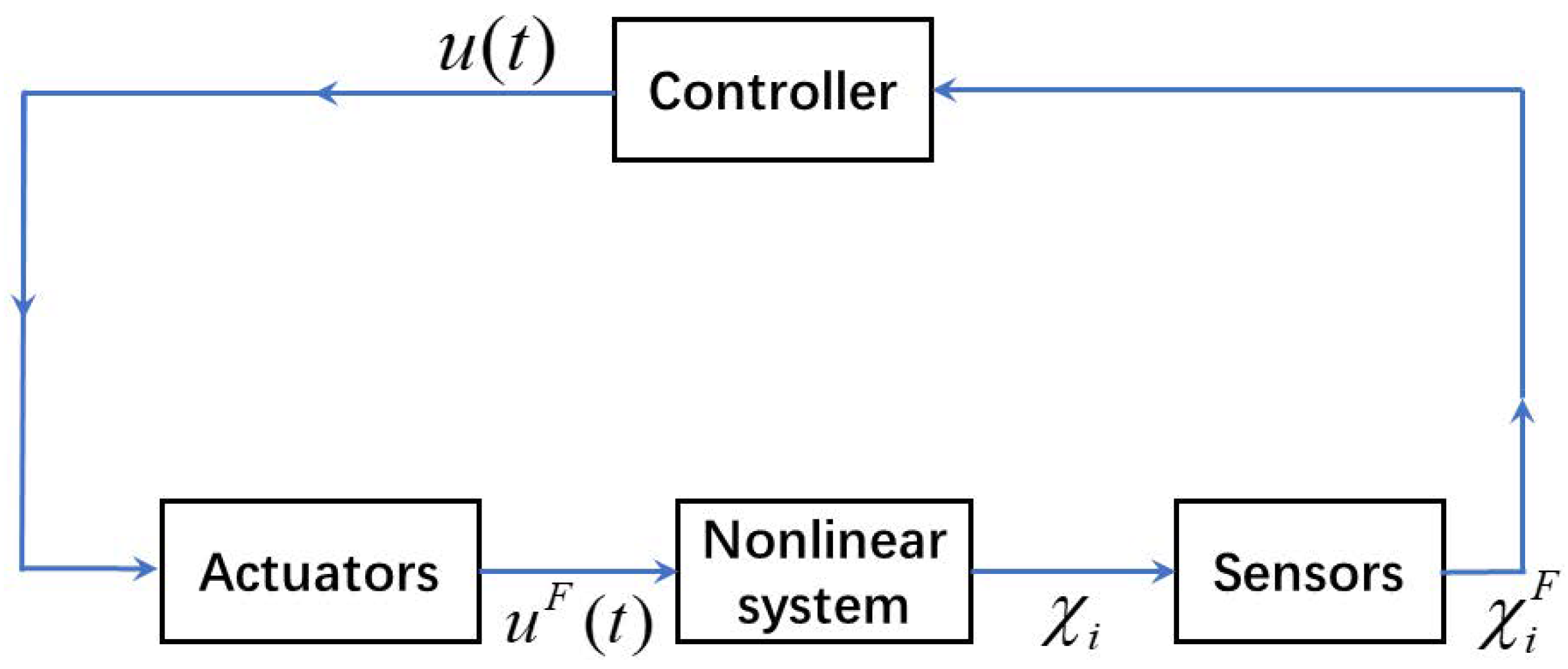
Figure 2.
Dynamical behavior of the fractional-order Chua-Hartley system.
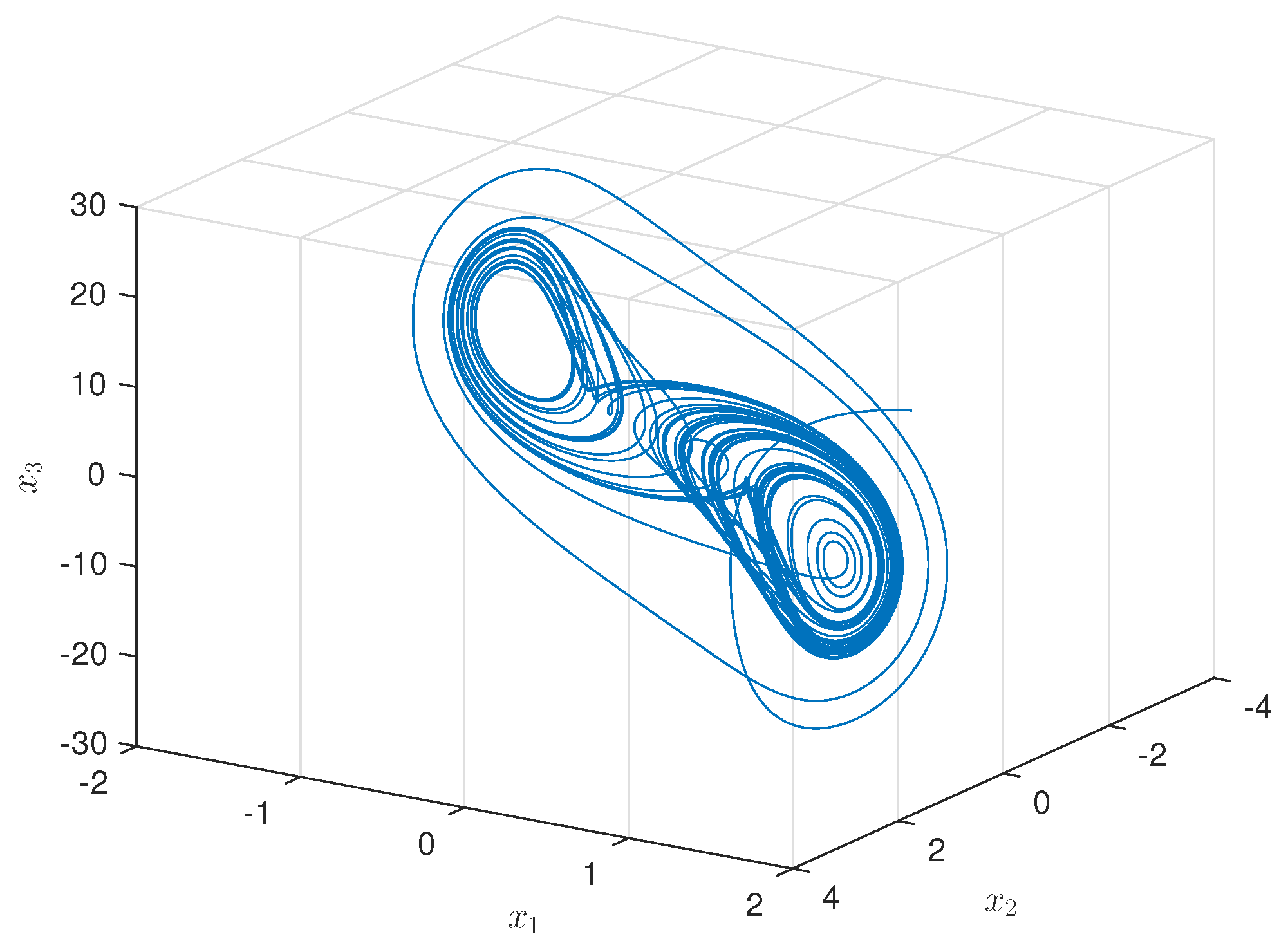
Figure 3.
The trajectories of y, and .
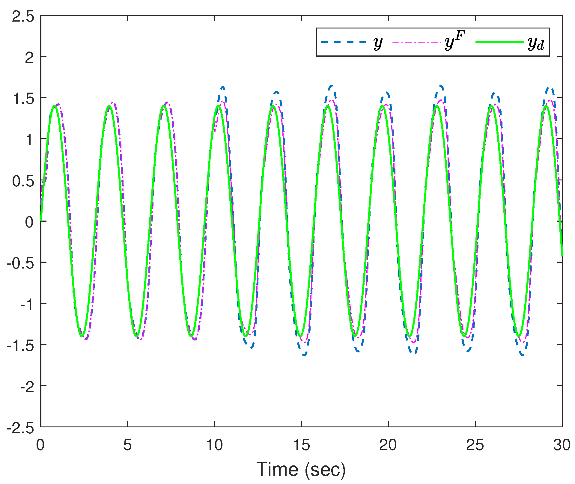
Figure 4.
The system states ().
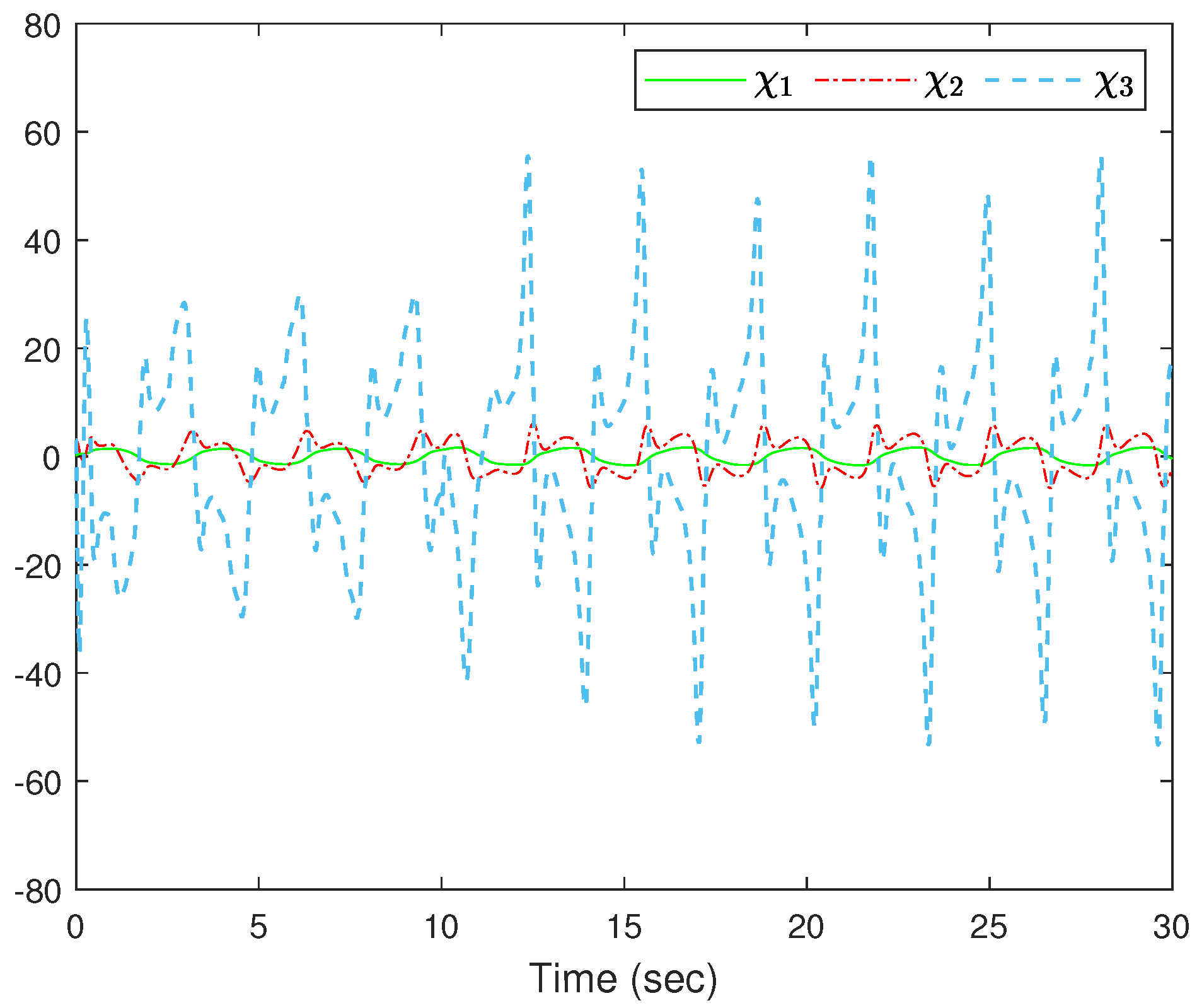
Figure 5.
The parameters and ().
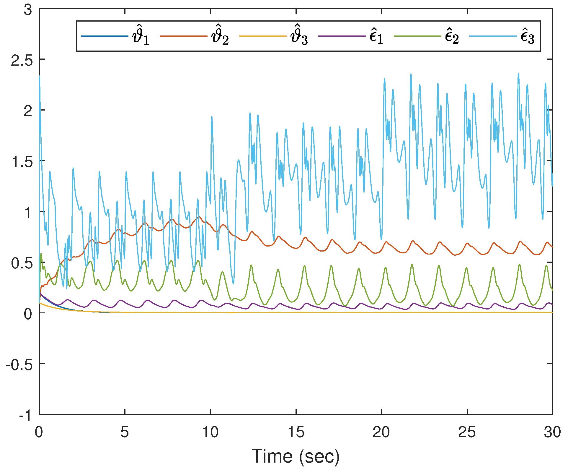
Figure 6.
The parameters and ().
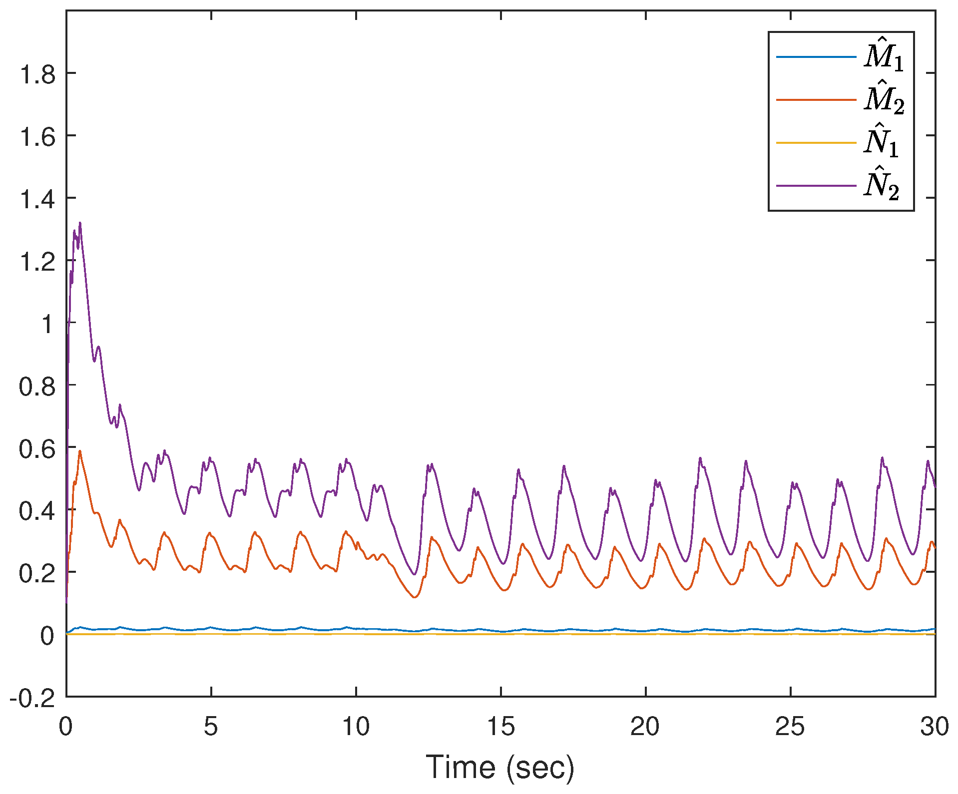
Figure 7.
The control input u.

Figure 8.
The trajectories of y, and in CASE 2.
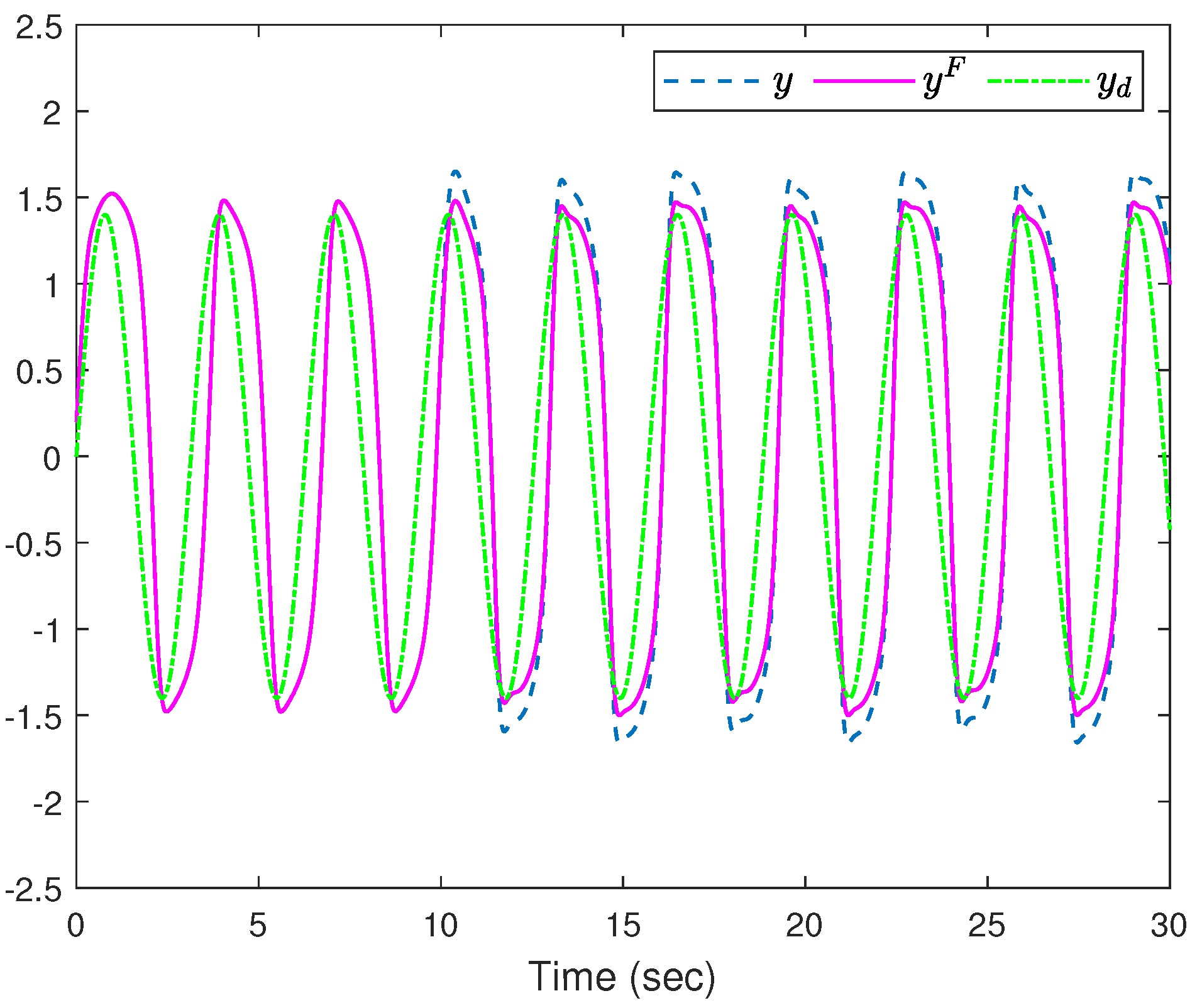
Figure 9.
The control input u in CASE 2.

Figure 10.
The trajectories of y, and using the strategy in [45].
Figure 10.
The trajectories of y, and using the strategy in [45].
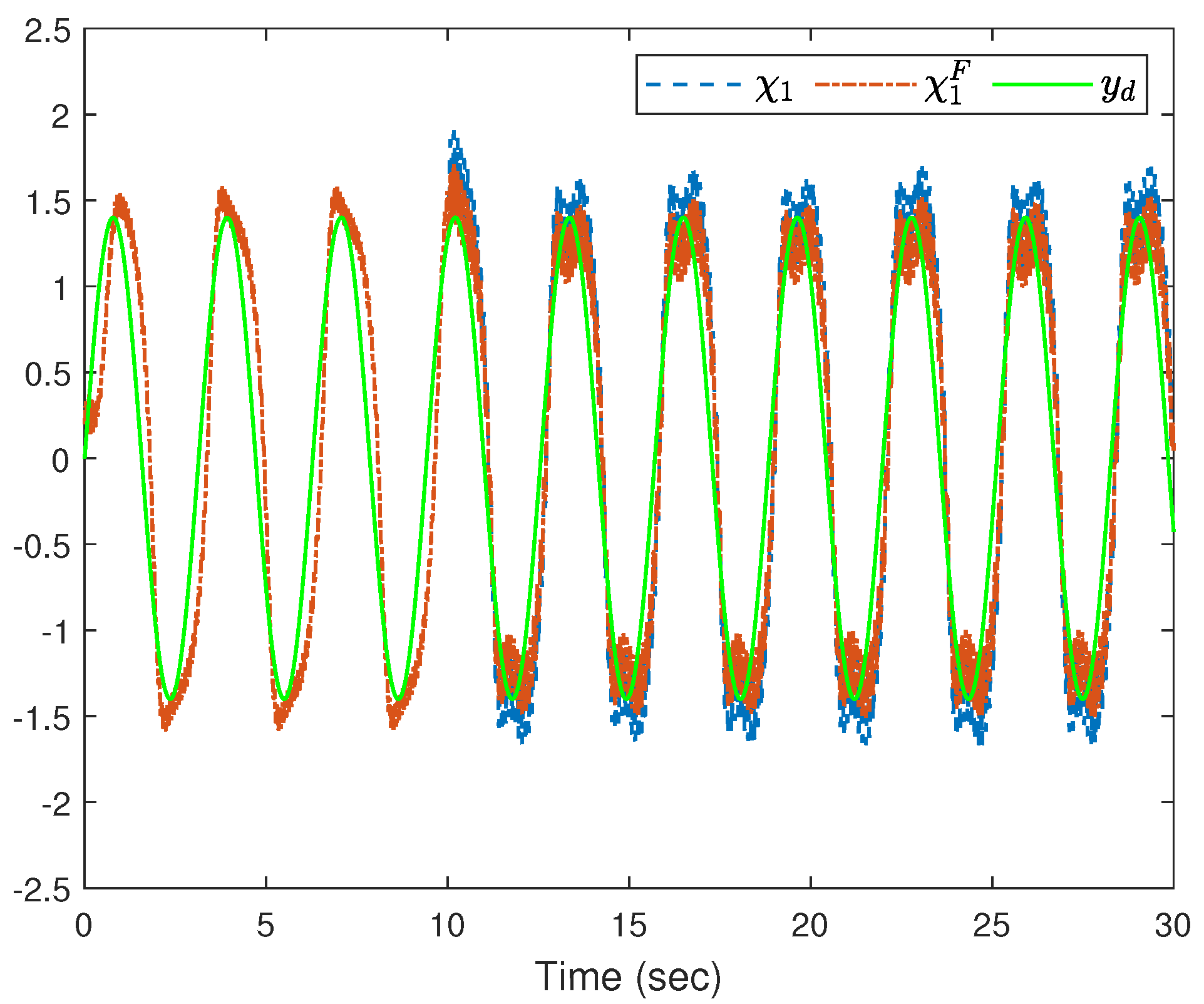
Figure 11.
The control input u using the strategy in [45].
Figure 11.
The control input u using the strategy in [45].

Table 1.
Fault Model.
| & | & | & | |
|---|---|---|---|
| Fault-free | 1 | 1 | 0 |
| Partial loss of effectiveness fault | >0 | <1 | 0 |
| Bias | 1 | 1 | |
| Total loss of effectiveness (TLOE) fault | 0 | 0 |
Disclaimer/Publisher’s Note: The statements, opinions and data contained in all publications are solely those of the individual author(s) and contributor(s) and not of MDPI and/or the editor(s). MDPI and/or the editor(s) disclaim responsibility for any injury to people or property resulting from any ideas, methods, instructions or products referred to in the content. |
© 2023 by the authors. Licensee MDPI, Basel, Switzerland. This article is an open access article distributed under the terms and conditions of the Creative Commons Attribution (CC BY) license (https://creativecommons.org/licenses/by/4.0/).
Share and Cite
MDPI and ACS Style
Sun, K.; Ma, Z.; Dong, G.; Gong, P. Adaptive Fuzzy Fault-Tolerant Control of Uncertain Fractional-Order Nonlinear Systems with Sensor and Actuator Faults. Fractal Fract. 2023, 7, 862. https://doi.org/10.3390/fractalfract7120862
AMA Style
Sun K, Ma Z, Dong G, Gong P. Adaptive Fuzzy Fault-Tolerant Control of Uncertain Fractional-Order Nonlinear Systems with Sensor and Actuator Faults. Fractal and Fractional. 2023; 7(12):862. https://doi.org/10.3390/fractalfract7120862
Chicago/Turabian StyleSun, Ke, Zhiyao Ma, Guowei Dong, and Ping Gong. 2023. "Adaptive Fuzzy Fault-Tolerant Control of Uncertain Fractional-Order Nonlinear Systems with Sensor and Actuator Faults" Fractal and Fractional 7, no. 12: 862. https://doi.org/10.3390/fractalfract7120862