Coupled Fixed Point and Hybrid Generalized Integral Transform Approach to Analyze Fractal Fractional Nonlinear Coupled Burgers Equation

Abstract

In this manuscript, the nonlinear Burgers equations are studied via a fractal fractional (FF) Caputo operator. The results of coupled fixed point theorems in cone metric space are used to discuss the uniqueness of solution to the proposed coupled equations. The solution of the proposed equation is computed via Natural transform associated with the Adomian decomposition method (NADM). The acquired results are graphically presented for some values of fractional order and fractal dimensions. The accuracy and consistency of the applied method is verified through error analysis.

1. Introduction

Partial differential equations (PDEs) have attracted researchers from different scientific fields due to their myriad of applications in natural and physical sciences [1,2,3]. There are several kinds of special PDEs in the literature [4,5]. J. M. Burgers [6] introduced the Burgers equation as a theoretical representation of turbulent fluid movement. As a simplified version of the Navier–Stokes equation, which simulates flow behavior, the Burgers equation is significant in a number of implications. Additionally, the Burgers equation is utilized as a model PDE to systematically create many of the core tools needed to investigate wider classes of PDEs in a reasonably simple environment. It has contributed significantly to the theoretical growth of stochastic PDEs with the inclusion of stochastic forcing. In addition, the Burgers equation has a normal form, which indicates that it at least intuitively captures the behavior of a considerably broader class of equations.

For many physical phenomena, including traffic, shock waves, turbulence issues, and continuous stochastic processes, the Burgers equation serves as a model example. It is one of a select group of nonlinear partial differential equations that have had some of their solutions analytically studied for various arbitrary beginning circumstances. These solutions frequently require infinite series, which for low values of the viscosity coefficient may converge extremely slowly. In addition, it may be used to evaluate different numerical methods. This is due to the wide range of applications of the Burgers equation [7,8,9,10].

Nowadays fractional calculus (FC) has attracted a number of researchers from various scientific fields. FC has the tendency to preserve short and long memory and provides the global evolution of a physical process. FC has many applications in the field of mathematical physics [11], biology [12], chemical reaction process [13], neural network [14,15], time-delay problems [16,17,18,19], etc. Due to its use in the study of over-driven explosions in gas [20], anomalous diffusion in semiconductor development [21], hereditary effects on nonlinear acoustic waves [22], nonlinear Markov processes, chaos propagation [23], and other fields, fractional Burgers equations have recently attracted a lot of attention. Through the use of the natural decomposition approach and nonsingular kernel derivatives, Aljahdaly et al. [24] have looked into the fractional-order Burgers equation. In the articles on Caputo–Fabrizio and Atangana–Baleanu derivatives, the two different kinds of fractional derivatives are utilized. To arrive at the solution of the equations, they applied the Natural transform to the fractional-order Burgers equation and then the Inverse Natural transform. With regard to the fractional view analysis of coupled Burgers equations, Nehad et al. [25] employ a cutting-edge analytical approach. The presented issues have undergone a Caputo–Fabrizio sense fractional analysis. The present strategy was first used to apply the Yang transformation to the given situation. The Adomian decomposition method is then used to produce the series form solution. For an appropriate selection of the fractional orders, Zhiping Mao and George Em Karniadakis [26] explored a novel fractional viscous Burgers equation with nonlinear fractional components that reduces to the classic Burgers equation. The fact that this equation can be solved using an application of the Hopf–Cole transformation to produce accurate solutions, which can be used to precisely quantify the numerical errors, makes it a particularly useful model for creating numerical techniques for nonlinear fractional conservation laws. Using effective methods, Khan et al. [27] recently presented the analytical solutions of the following systems of two-dimensional fractional Burgers equations.

$$\begin{array}{c}\hfill \left\{\begin{array}{c}{}_0^C{D}_{\mathsf{t}}^{\alpha }\Phi (\theta ,\zeta ,\mathsf{t})={\Phi }_{\theta \theta }+{\Phi }_{\zeta \zeta }-\Phi {\Phi }_{\theta }-\Psi {\Phi }_{\zeta },\hfill \\ {}_0^C{D}_{\mathsf{t}}^{\alpha }\Psi (\theta ,\zeta ,\mathsf{t})={\Psi }_{\theta \theta }+{\Psi }_{\zeta \zeta }-\Phi {\Psi }_{\theta }-\Psi {\Psi }_{\zeta },\hfill \end{array}\right.\end{array}$$

(1)

with initial condition $\Phi (\theta ,\zeta ,0)=\theta +\zeta$, $\Psi (\theta ,\zeta ,0)=\theta -\zeta$ and

$$\begin{array}{c}\hfill \left\{\begin{array}{c}{}_0^C{D}_{\mathsf{t}}^{\alpha }\Phi (\theta ,\mathsf{t})=2\Phi {\Phi }_{\theta }-{\Phi }_{\theta \theta }+{(\Phi \Psi )}_{\theta },\hfill \\ {}_0^C{D}_{\mathsf{t}}^{\alpha }\Psi (\theta ,\mathsf{t})=-2\Psi {\Psi }_{\theta }-{\Psi }_{\theta \theta }-{(\Phi \Psi )}_{\theta },\hfill \end{array}\right.\end{array}$$

(2)

where $0<\alpha \le 1$ and initial conditions are $\Phi (\theta ,0)=sin\left(\theta \right)$, $\Psi (\theta ,0)=-sin\left(\theta \right)$.

A novel class of fractional derivatives with a power law kernel, known as fractal-fractional (FF) derivatives, has several applications in practical issues. This operator is utilized in this type of fluid flow for the first time. The main benefit of this operator is that it makes it possible to create models that describe systems with memory effects considerably more accurately. Additionally, there are numerous issues in the actual world where it is vital to understand how much information the system contains. We explain some applications of FF operators in different areas of science. Saifullah et al. investigated the nonlinear Drinfeld–Sokolov–Wilson system using an FF operator [28]. Gulalai et al. studied a fractal fractional analysis-modified KdV equation under different FF operators [29]. There are several applications of FF operators in the literature [30,31,32].

The motivation behind employing the FF Caputo operator lies in its unique ability to describe and capture long-range dependencies, nonlocal interactions, and complex behaviors within the system. By incorporating this operator into the study of Burgers equations, we can potentially overcome the limitations of traditional approaches and gain a deeper understanding of the underlying dynamics. The FF Caputo operator also gives a means to model and illustrate systems that exhibit nonlocal interactions, long-range dependencies, and memory impacts. These aspects are often present in different natural and engineered systems, such as turbulent fluid flows or complex biological processes. Hence, using this operator in the analysis of Burgers equations enables us to enhance the limitations of traditional techniques and escalate our ability to explain and predict real-world phenomena more precisely. This enhances our ability to describe and forecast the evolution of systems governed by Burgers equations, leading to more precise and reliable outcomes. The use of the FF Caputo operator in studying Burgers equations studies gaps in the field by overcoming limitations of traditional methods. Conventional techniques often struggle to capture nonlocal interactions, memory effects, and complex scaling features accurately. By introducing the fractal fractional Caputo operator, this approach bridges these gaps and provides a more comprehensive framework for analyzing and solving Burgers equations. Motivated by the above literature, we consider Equations (1) and (2) using the Caputo FF operator as:

$$\begin{array}{c}\hfill \left\{\begin{array}{c}{}_0^C{D}_{\mathsf{t}}^{\alpha ,\beta }\Phi (\theta ,\zeta ,\mathsf{t})={\Phi }_{\theta \theta }+{\Phi }_{\zeta \zeta }-\Phi {\Phi }_{\theta }-\Psi {\Phi }_{\zeta },\hfill \\ {}_0^C{D}_{\mathsf{t}}^{\alpha ,\beta }\Psi (\theta ,\zeta ,\mathsf{t})={\Psi }_{\theta \theta }+{\Psi }_{\zeta \zeta }-\Phi {\Psi }_{\theta }-\Psi {\Psi }_{\zeta },\hfill \end{array}\right.\end{array}$$

(3)

with initial condition $\Phi (\theta ,\zeta ,0)=\theta +\zeta$, $\Psi (\theta ,\zeta ,0)=\theta -\zeta$. In addition,

$$\begin{array}{c}\hfill \left\{\begin{array}{c}{}_0^C{D}_{\mathsf{t}}^{\alpha ,\beta }\Phi (\theta ,\mathsf{t})=2\Phi {\Phi }_{\theta }-{\Phi }_{\theta \theta }+{(\Phi \Psi )}_{\theta },\hfill \\ {}_0^C{D}_{\mathsf{t}}^{\alpha ,\beta }\Psi (\theta ,\mathsf{t})=-2\Psi {\Psi }_{\theta }-{\Psi }_{\theta \theta }-{(\Phi \Psi )}_{\theta },where0<\alpha ,\beta \le 1,\hfill \end{array}\right.\end{array}$$

(4)

with initial condition $\Phi (\theta ,0)=sin\left(\theta \right)$, $\Psi (\theta ,0)=-sin\left(\theta \right)$. where ${}_0^C{D}_{\mathsf{t}}^{\alpha ,\beta }$ denotes the Caputo FF operator, which we define in the following section.

In this manuscript, we will solve (1) and (2) with the fractal fractional operator using the Natural transform decomposition approach. Utilizing some fixed point results, it is investigated if the solutions to the provided issues exist and are unique. The solutions to some examples are provided to demonstrate the validity and applicability of the suggested strategies.

2. Preliminaries

In this section, we give some basic notions of Caputo FF operators and Natural transform (NT). Let $\lambda \left(\mathsf{t}\right)$ be fractal differential and continuous on an open interval $(m_1,m_2)$ and $\frac{d}{d{\upsilon }^{\beta }}={lim}_{t\to \upsilon }\frac{\mathsf{t}\left(t\right)-\mathsf{t}\left(\upsilon \right)}{t^{\beta }-{\upsilon }^{\beta }}$.

Definition 1 ([33]).

For $\alpha ,\beta \in (0,1]$, the Caputo FF derivative is expressed as:

$$\begin{array}{ccc}\hfill {}_0^C{D}_{\mathsf{t}}^{\alpha ,\beta }\lambda \left(\mathsf{t}\right)& =& \frac{1}{\Gamma (1-\alpha )}{\int }_0^{\mathsf{t}}{(\mathsf{t}-\upsilon )}^{-\alpha }\frac{d}{d{\upsilon }^{\beta }}\lambda \left(\upsilon \right)d\upsilon ,\hfill \end{array}$$

where α and β represent the fractional order and fractal dimension, respectively.

Definition 2 ([33]).

For $0<\alpha ,\beta \le 1$, the FF integral is given by:

$${\mathcal{I}}_{0,\mathsf{t}}^{\alpha ,\beta }\lambda \left(\mathsf{t}\right)=\frac{\beta }{\Gamma \left(\alpha \right)}{\int }_0^{\mathsf{t}}{(t-\upsilon )}^{\alpha -1}{\upsilon }^{\beta -1}\lambda \left(\upsilon \right)d\upsilon .$$

Definition 3 ([34]).

The NT of the function $\lambda \left(\mathsf{t}\right)$ is presented by $N\left[\lambda \right(\mathsf{t}\left)\right]$ and with variables S and ℘ is defined by:

$$N\left[\lambda \left(\mathsf{t}\right)\right]=R(S,\wp )={\int }_{-\infty }^{\infty }{e}^{-S\mathsf{t}}\lambda (\wp \mathsf{t})dt,S,\wp \in (-\infty ,\infty ).$$

Definition 4 ([35]).

The NT of ${}_0^C{D}_{\mathsf{t}}^{\alpha }\lambda \left(\mathsf{t}\right)$ is defined as:

$$N\left[{}_0^C{D}_{\mathsf{t}}^{\alpha }\lambda \left(\mathsf{t}\right)\right]=\frac{S^{\alpha }}{{\wp }^{\alpha }}N\left[\lambda \left(\mathsf{t}\right)\right]-\sum _{k=0}^{n-1}\frac{S^{\alpha -(k+1)}}{{\wp }^{\alpha -k}}{\left[D^k\lambda \left(\mathsf{t}\right)\right]}_{\mathsf{t}=0}.$$

(5)

Definition 5 ([36]).

Let $\mathcal{E}$ denote a Banach space with norm $\parallel .\parallel$ and $\mathcal{P}$⊆$\mathcal{E}$. Then, $\mathcal{P}$ is said to be a cone if:

• $\mathcal{P}\ne \varnothing$, closed, and $\mathcal{P}\ne \left\{\varpi \right\}$, where ϖ denotes zero vector in $\mathcal{E}$.
• $\forall b,s\ge 0$ and $\mathsf{x},\mathsf{y}\in \mathcal{P}$ then $b\mathsf{x}+s\mathsf{y}\in \mathcal{P}$.
• If $\mathsf{x}\in \mathcal{P}$ and $-\mathsf{x}\in \mathcal{P}$ then $\mathsf{x}=\varpi$.

Let $\mathcal{P}$ be a cone in a Banach space $\mathcal{E}$; then, a partial ordering ⪯ with respect to $\mathcal{P}$ is defined as: $\mathsf{x}⪯\mathsf{y}\iff \mathsf{y}-\mathsf{x}\in \mathcal{P}$. The cone $\mathcal{P}$ is said to be normal if ∃$k>0$, such that ∀$\mathsf{x},\mathsf{y}\in \mathcal{E}$, we have $\varpi ⪯\mathsf{x}⪯\mathsf{y}\Rightarrow \parallel \mathsf{x}\parallel \le k\parallel \mathsf{y}\parallel$.

Definition 6 ([36]).

A cone metric space is said to be an ordered pair $(\mathcal{X},\mathsf{d})$ and $\mathsf{d}:\mathcal{X}\times \mathcal{X}\to \mathcal{E}$ is a mapping which satisfies:

• $\mathsf{d}(\mathsf{x},\mathsf{y})\in \mathcal{P}$, that is $\varpi ⪯d(\mathsf{x},\mathsf{y})$, ∀$\mathsf{x},\mathsf{y}\in \mathcal{X}$, and $\mathsf{d}(\mathsf{x},\mathsf{y})=\varpi$ if $\mathsf{x}=\mathsf{y}$.
• $\mathsf{d}(\mathsf{x},\mathsf{y})=\mathsf{d}(\mathsf{y},\mathsf{x})$∀$\mathsf{x},\mathsf{y}\in \mathcal{X}$.
• $\mathsf{d}(\mathsf{x},\mathsf{y})⪯\mathsf{d}(\mathsf{x},z)+\mathsf{d}(z,\mathsf{y})$∀$\mathsf{x},\mathsf{y},z\in \mathcal{X}$.

3. Existence of Unique Solution

In this part, the notions of fixed point theory are used to discuss the results concerned with the existence of a unique solution of Equation (2). For Equation (3), the readers may derive the same results. For these purposes first, we recall the following result:

Theorem 1 ([37]).

Suppose $\mathcal{E}$ is the real Banach space and the cone $\mathcal{P}$ of $\mathcal{E}$ is normal. Furthermore, $\mathcal{F}:\left[0,1\right]\times \left[0,1\right]\to \mathcal{E}$ and ${\mathcal{F}}_1:\left[0,1\right]\times \left[0,1\right]\to \mathcal{E}$ are completely continuous. If there exists $0<\kappa <1$ such that

$$\begin{array}{ccc}\hfill \parallel \mathcal{F}(\theta ,\zeta )-{\mathcal{F}}_1(\zeta ,\theta )\parallel & \le & \kappa \parallel \theta -\zeta \parallel ,\hfill \end{array}$$

$\forall (\theta ,\zeta )\in \left[0,1\right]\times \left[0,1\right]$. Then, $\mathcal{F}$ has exactly one fixed point.

Now, we can write Equation (3) as:

$$\begin{array}{ccc}\hfill {}_0{D}_{\mathsf{t}}^{\alpha }\Psi & =& \beta {\mathsf{t}}^{\beta -1}\mathcal{A}(\mathsf{t},\theta ,\zeta ,\Phi ,\Psi ),\hfill \\ \hfill {}_0{D}_{\mathsf{t}}^{\alpha }\Phi & =& \beta {\mathsf{t}}^{\beta -1}{\mathcal{A}}_1(\mathsf{t},\theta ,\zeta ,\Psi ,\Phi ),\hfill \end{array}$$

with initial condition $\Phi (\theta ,\zeta ,0)={\Phi }_{\circ }$ , $\Psi (\theta ,\zeta ,0)={\Psi }_{\circ }$ and $\mathcal{A}$ and ${\mathcal{A}}_1$ denote the right-hand side of Equation (3). Applying fractional integration, we have

$$\begin{array}{ccc}\hfill \Phi (\mathsf{t},\theta ,\zeta )& =& {\Phi }_{\circ }+\frac{\beta }{\Gamma \left(\alpha \right)}{\int }_0^{\mathsf{t}}{\left(\mathsf{t}-\upsilon \right)}^{\alpha -1}{\upsilon }^{\beta -1}\mathcal{A}(\upsilon ,\theta ,\zeta ,\Phi ,\Psi )d\upsilon ,\hfill \\ \hfill \Psi (\mathsf{t},\theta ,\zeta )& =& {\Psi }_{\circ }+\frac{\beta }{\Gamma \left(\alpha \right)}{\int }_0^{\mathsf{t}}{\left(\mathsf{t}-\upsilon \right)}^{\alpha -1}{\upsilon }^{\beta -1}{\mathcal{A}}_1(\upsilon ,\theta ,\zeta ,\Psi ,\Phi )d\upsilon .\hfill \end{array}$$

Consider

$$\begin{array}{c}\hfill \left\{\begin{array}{c}\Phi (\mathsf{t},\theta ,\zeta )={\Phi }_{\circ }+\frac{\beta }{\Gamma \left(\alpha \right)}{\int }_0^{\mathsf{t}}{\left(\mathsf{t}-\upsilon \right)}^{\alpha -1}{\upsilon }^{\beta -1}\mathcal{A}(\upsilon ,\theta ,\zeta ,\Phi ,\Psi )d\upsilon =\mathcal{F}\left(\mathsf{t},\theta ,\zeta ,\Phi ,\Psi \right)\hfill \\ \Psi (\mathsf{t},\theta ,\zeta )={\Psi }_{\circ }+\frac{\beta }{\Gamma \left(\alpha \right)}{\int }_0^{\mathsf{t}}{\left(\mathsf{t}-\upsilon \right)}^{\alpha -1}{\upsilon }^{\beta -1}{\mathcal{A}}_1(\upsilon ,\theta ,\zeta ,\Psi ,\Phi )d\upsilon ={\mathcal{F}}_1\left(\mathsf{t},\theta ,\zeta ,\Psi ,\Phi \right).\hfill \end{array}\right.\end{array}$$

(6)

The following theorem shows that there exists a unique solution to the system (6).

Theorem 2. 

Let $\left(\mathcal{C},\mathsf{d}\right)$ be the space of all continuous function $\mathsf{d}(\theta ,\zeta )=sup|\theta -\zeta |=\parallel \theta -\zeta \parallel$. In addition, $\mathcal{F}:\mathcal{C}\times \mathcal{C}\to \mathcal{C}$ and ${\mathcal{F}}_1:\mathcal{C}\times \mathcal{C}\to \mathcal{C}$. Then, the system (6) has a unique solution if the following conditions hold

i.

$\mathcal{P}$ is a normal cone and $\mathcal{F}$ and ${\mathcal{F}}_1$ are completely continuous.

ii.

The operators $\frac{{\partial }^2}{\partial {\theta }^2},\frac{{\partial }^2}{\partial {\zeta }^2},\frac{\partial }{\partial \theta },\frac{\partial }{\partial \zeta }$ satisfied the Lipschitz condition.

iii.

$\parallel \Phi \parallel \le ħ$ and $\parallel \Psi \parallel \le \hslash ,$ where $ħ,\hslash >0$ and $\parallel {\Phi }_{\circ }-{\Psi }_{\circ }\parallel \le \frac{\parallel \Phi -\Psi \parallel }{2}$ for all $(\theta ,\zeta )\in [0,1]$.

iv.

$\frac{\beta }{\Gamma \left(\alpha \right)}{\int }_0^{\mathsf{t}}{\left(\mathsf{t}-\upsilon \right)}^{\alpha -1}{\upsilon }^{\beta -1}d\upsilon \le 1$ and $0<\left(\frac{1}{2}+\rho +\varrho +ħ\sigma +\hslash \varsigma \right)=\varpi <1$.

Proof. 

Since for all $(\theta ,\zeta )\in \left[0,1\right]\times \left[0,1\right]$, we have

$$\begin{array}{ccc}\hfill |\mathcal{F}(\mathsf{t},\theta ,\zeta ,\Phi ,\Psi )-{\mathcal{F}}_1(\mathsf{t},\theta ,\zeta ,\Psi ,\Phi )|& =& \left|{\Phi }_{\circ }+\frac{\beta }{\Gamma \left(\alpha \right)}{\int }_0^{\mathsf{t}}{\left(\mathsf{t}-\upsilon \right)}^{\alpha -1}{\upsilon }^{\beta -1}\mathcal{A}(\upsilon ,\theta ,\zeta ,\Phi ,\Psi )d\upsilon \right.\hfill \\ & & \left.-{\Psi }_{\circ }-\frac{\beta }{\Gamma \left(\alpha \right)}{\int }_0^{\mathsf{t}}{\left(\mathsf{t}-\upsilon \right)}^{\alpha -1}{\upsilon }^{\beta -1}{\mathcal{A}}_1(\upsilon ,\theta ,\zeta ,\Psi ,\Phi )d\upsilon \right|\hfill \\ & \le & |{\Phi }_{\circ }-{\Psi }_{\circ }|+\frac{\beta }{\Gamma \left(\alpha \right)}{\int }_0^{\mathsf{t}}{\left(\mathsf{t}-\upsilon \right)}^{\alpha -1}{\upsilon }^{\beta -1}\hfill \\ & & \times \left|\mathcal{A}(\mathsf{t},\theta ,\zeta ,\Phi ,\Psi )-{\mathcal{A}}_1(\mathsf{t},\theta ,\zeta ,\Psi ,\Phi )\right|d\upsilon \hfill \\ & =& |{\Phi }_{\circ }-{\Psi }_{\circ }|+\frac{\beta }{\Gamma \left(\alpha \right)}{\int }_0^{\mathsf{t}}{\left(\mathsf{t}-\upsilon \right)}^{\alpha -1}{\upsilon }^{\beta -1}\hfill \\ & & \times \left|{\Phi }_{\theta \theta }+{\Phi }_{\zeta \zeta }-\Phi {\Phi }_{\theta }-\Psi {\Phi }_{\zeta }\right.\hfill \\ & & \left.-{\Psi }_{\theta \theta }-{\Psi }_{\zeta \zeta }+\Phi {\Psi }_{\theta }+\Psi {\Psi }_{\zeta }\right|d\upsilon \hfill \end{array}$$

$$\begin{array}{ccc}\hfill & =& |{\Phi }_{\circ }-{\Psi }_{\circ }|+\frac{\beta }{\Gamma \left(\alpha \right)}{\int }_0^{\mathsf{t}}{\left(\mathsf{t}-\upsilon \right)}^{\alpha -1}{\upsilon }^{\beta -1}\left|\frac{{\partial }^2}{\partial {\theta }^2}(\Phi -\Psi )+\frac{{\partial }^2}{\partial {\zeta }^2}(\Phi -\Psi )\right.\hfill \\ & & \left.-\Phi \frac{\partial }{\partial \theta }(\Phi -\Psi )-\Psi \frac{\partial }{\partial \zeta }(\Phi -\Psi )\right|d\upsilon \hfill \\ & \le & |{\Phi }_{\circ }-{\Psi }_{\circ }|+\frac{\beta }{\Gamma \left(\alpha \right)}{\int }_0^{\mathsf{t}}{\left(\mathsf{t}-\upsilon \right)}^{\alpha -1}{\upsilon }^{\beta -1}\left[\left|\frac{{\partial }^2}{\partial {\theta }^2}(\Phi -\Psi )\right|+\left|\frac{{\partial }^2}{\partial {\zeta }^2}(\Phi -\Psi )\right|\right.\hfill \\ & & \left.+|\Phi |\left|\frac{\partial }{\partial \theta }(\Phi -\Psi )\right|+|\Psi |\left|\frac{\partial }{\partial \zeta }(\Phi -\Psi )\right|\right]d\upsilon \hfill \\ & \le & |{\Phi }_{\circ }-{\Psi }_{\circ }|+\frac{\beta }{\Gamma \left(\alpha \right)}{\int }_0^{\mathsf{t}}{\left(\mathsf{t}-\upsilon \right)}^{\alpha -1}{\upsilon }^{\beta -1}\left(\rho |\Phi -\Psi |+\varrho |\Phi -\Psi |+\sigma |\Phi ||\Phi -\Psi |+\varsigma |\Psi ||\Phi -\Psi |\right)d\upsilon ,\hfill \end{array}$$

where $\rho ,\varrho ,\sigma$ and $\varsigma$ are Lipschitz constants for the operators $\frac{{\partial }^2}{\partial {\theta }^2},\frac{{\partial }^2}{\partial {\zeta }^2},\frac{\partial }{\partial \theta },\frac{\partial }{\partial \zeta }$. Therefore,

$$\begin{array}{ccc}\hfill sup|\mathcal{F}(\mathsf{t},\theta ,\zeta ,\Phi ,\Psi )-{\mathcal{F}}_1(\mathsf{t},\theta ,\zeta ,\Psi ,\Phi )|& =& sup\left(|{\Phi }_{\circ }-{\Psi }_{\circ }|+\frac{\beta }{\Gamma \left(\alpha \right)}{\int }_0^{\mathsf{t}}{\left(\mathsf{t}-\upsilon \right)}^{\alpha -1}{\upsilon }^{\beta -1}\right.\hfill \\ & & \left.\left(\rho |\Phi -\Psi |+\varrho |\Phi -\Psi |+\sigma |\Phi ||\Phi -\Psi |+\varsigma |\Psi ||\Phi -\Psi |\right)d\upsilon \right)\hfill \\ & \le & sup|{\Phi }_{\circ }-{\Psi }_{\circ }|+\frac{\beta }{\Gamma \left(\alpha \right)}{\int }_0^{\mathsf{t}}{\left(\mathsf{t}-\upsilon \right)}^{\alpha -1}{\upsilon }^{\beta -1}\hfill \\ & & \left(\rho sup|\Phi -\Psi |+\varrho sup|\Phi -\Psi |+\sigma \parallel \Phi \parallel sup|\Phi -\Psi |\right.\hfill \\ & & \left.+\varsigma \parallel \Psi \parallel sup|\Phi -\Psi |\right)d\upsilon \hfill \\ & =& \parallel {\Phi }_{\circ }-{\Psi }_{\circ }\parallel +\frac{\beta }{\Gamma \left(\alpha \right)}{\int }_0^{\mathsf{t}}{\left(\mathsf{t}-\upsilon \right)}^{\alpha -1}{\upsilon }^{\beta -1}\hfill \\ & & \left(\rho \parallel \Phi -\Psi \parallel +\varrho \parallel \Phi -\Psi \parallel +ħ\sigma \parallel \Phi -\Psi \parallel +\hslash \varsigma \parallel \Phi -\Psi \parallel \right)d\upsilon \hfill \\ & \le & \frac{\parallel \Phi -\Psi \parallel }{2}+\left(\rho \parallel \Phi -\Psi \parallel +\varrho \parallel \Phi -\Psi \parallel +ħ\sigma \parallel \Phi -\Psi \parallel +\hslash \varsigma \parallel \Phi -\Psi \parallel \right)\hfill \\ & & \frac{\beta }{\Gamma \left(\alpha \right)}{\int }_0^{\mathsf{t}}{\left(\mathsf{t}-\upsilon \right)}^{\alpha -1}{\upsilon }^{\beta -1}d\upsilon \hfill \\ & \le & \frac{\parallel \Phi -\Psi \parallel }{2}+\left(\rho \parallel \Phi -\Psi \parallel +\varrho \parallel \Phi -\Psi \parallel +ħ\sigma \parallel \Phi -\Psi \parallel +\hslash \varsigma \parallel \Phi -\Psi \parallel \right)\hfill \\ & =& \left(\frac{1}{2}+\rho +\varrho +ħ\sigma +\hslash \varsigma \right)\parallel \Phi -\Psi \parallel \hfill \\ & =& \varpi \parallel \Phi -\Psi \parallel .\hfill \end{array}$$

Consequently

$$\begin{array}{ccc}\hfill \parallel \mathcal{F}(\mathsf{t},\theta ,\zeta ,\Phi ,\Psi )-{\mathcal{F}}_1(\mathsf{t},\theta ,\zeta ,\Psi ,\Phi )\parallel & \le & \varpi \parallel \Phi -\Psi \parallel .\hfill \end{array}$$

Therefore, from Theorem 1, there exists exactly one fixed point of $\mathcal{F}$. Hence, the system (3) has exactly one fixed point. So, the solution of (3) is unique. □

4. Solution Strategy

Consider the following nonlinear general partial differential equation with an FF operator as

$$\begin{array}{ccc}\hfill {}_0^C{D}_{\mathsf{t}}^{\alpha ,\beta }\Phi (\theta ,\zeta ,\mathsf{t})& =& -\psi (\theta ,\zeta )\Phi (\theta ,\zeta ,\mathsf{t})-\phi (\theta ,\zeta )\Phi (\theta ,\zeta ,\mathsf{t})+\eta (\theta ,\zeta ,\mathsf{t}),\hfill \\ \hfill {}_0^C{D}_{\mathsf{t}}^{\alpha ,\beta }\Psi (\theta ,\zeta ,\mathsf{t})& =& -\psi (\theta ,\zeta )\Psi (\theta ,\zeta ,\mathsf{t})-\phi (\theta ,\zeta )\Psi (\theta ,\zeta ,\mathsf{t})+\eta (\theta ,\zeta ,\mathsf{t}),\hfill \end{array}$$

(7)

where $\mathsf{t}>0$, $0<\alpha ,\beta \le 1$, $\psi \left(\theta \right)$ is a general linear term and $\phi \left(\theta \right)$ is a nonlinear term. Now, from Equation (2), we have

$$\begin{array}{ccc}\hfill {}_0^C{D}_{\mathsf{t}}^{\alpha }\Phi (\theta ,\zeta ,\mathsf{t})& =& \beta {\mathsf{t}}^{\beta -1}\left[-\psi (\theta ,\zeta )\Phi (\theta ,\zeta ,\mathsf{t})-\phi (\theta ,\zeta )\Phi (\theta ,\zeta ,\mathsf{t})+\eta (\theta ,\zeta ,\mathsf{t})\right].\hfill \end{array}$$

Applying Natural transform, we obtain

$$\begin{array}{ccc}\hfill \frac{S^{\alpha }}{{\rho }^{\alpha }}N\left[\Phi \right]-\frac{S^{\alpha -1}}{{\rho }^{\alpha }}\Phi (\theta ,\zeta ,0)& =& N\left[\beta {\mathsf{t}}^{\beta -1}\left(-\psi (\theta ,\zeta )\Phi (\theta ,\zeta ,\mathsf{t})-\phi (\theta ,\zeta )\Phi (\theta ,\zeta ,\mathsf{t})+\eta (\theta ,\zeta ,\mathsf{t})\right)\right].\hfill \end{array}$$

Or

$$\begin{array}{ccc}\hfill N\left[\Phi \right]& =& \frac{1}{S}\Phi (\theta ,\zeta ,0)+\frac{{\rho }^{\alpha }}{S^{\alpha }}N\left[\beta {\mathsf{t}}^{\beta -1}\left(-\psi (\theta ,\zeta )\Phi (\theta ,\zeta ,\mathsf{t})-\phi (\theta ,\zeta )\lambda (\theta ,\zeta ,\mathsf{t})+\eta (\theta ,\zeta ,\mathsf{t})\right)\right].\hfill \end{array}$$

Now, applying the inverse of the Natural transform, we have

$$\begin{array}{ccc}\hfill \Phi (\theta ,\zeta ,\mathsf{t})& =& \Phi (\theta ,\zeta ,0)+N^{-1}\left[\frac{{\rho }^{\alpha }}{S^{\alpha }}N\left(\beta {\mathsf{t}}^{\beta -1}\left(-\psi (\theta ,\zeta )\Phi (\theta ,\zeta ,\mathsf{t})-\phi (\theta ,\zeta )\Phi (\theta ,\zeta ,\mathsf{t})+\eta (\theta ,\zeta ,\mathsf{t})\right)\right)\right].\hfill \end{array}$$

(8)

Then, the series solution is given by

$$\begin{array}{ccc}\hfill \Phi (\theta ,\zeta ,\mathsf{t})& =& \sum _{\mathrm{h}=0}^{\infty }{\Phi }_{\mathrm{h}}(\theta ,\zeta ,\mathsf{t}).\hfill \end{array}$$

The nonlinear term is decomposed by Adomian polynomial as

$$A_{\mathrm{h}}=\frac{1}{\mathrm{h}!}\frac{d^{\mathrm{h}}}{d{\rho }^{\mathrm{h}}}{\left[\zeta \left(\sum _{i=0}^{\mathrm{h}}{\rho }^i{\Phi }_i\right)\right]}_{\rho =0},h=0,1,2,...$$

So, Equation (8) becomes

$$\begin{array}{ccc}\hfill \sum _{\mathrm{h}=0}^{\infty }{\Phi }_{\mathrm{h}}(\theta ,\zeta ,\mathsf{t})& =& \Phi (\theta ,\zeta ,0)+N^{-1}\left[\frac{{\rho }^{\alpha }}{S^{\alpha }}N\left[\beta {\mathsf{t}}^{\beta -1}\left(-\psi (\theta ,\zeta )\sum _{h=0}^{\infty }\Phi (\theta ,\zeta ,\mathsf{t})-\sum _{\mathrm{h}=0}^{\infty }{A}_{\mathrm{h}}\sum _{\mathrm{h}=0}^{\infty }{\Phi }_{\mathrm{h}}+\eta (\theta ,\zeta ,\mathsf{t})\right)\right]\right].\hfill \end{array}$$

So, we can write the first few terms of the series as

$$\begin{array}{c}{\Phi }_{\circ }(\theta ,\zeta ,\mathsf{t})=\Phi (\theta ,\zeta ,0)\hfill \\ {\Phi }_1(\theta ,\zeta ,\mathsf{t})=N^{-1}\left[\frac{{\rho }^{\alpha }}{S^{\alpha }}N\left[\beta {\mathsf{t}}^{\beta -1}\left(-\psi (\theta ,\zeta ){\Phi }_{\circ }(\theta ,\zeta ,\mathsf{t})-A_{\circ }{\Phi }_{\circ }(\theta ,\zeta ,\mathsf{t})+\eta (\theta ,\zeta ,\mathsf{t})\right)\right]\right],\hfill \\ {\Phi }_2(\theta ,\zeta ,\mathsf{t})=N^{-1}\left[\frac{{\rho }^{\alpha }}{S^{\alpha }}N\left[\beta {\mathsf{t}}^{\beta -1}\left(-\psi (\theta ,\zeta ){\Phi }_1(\theta ,\zeta ,\mathsf{t})-A_1{\Phi }_1(\theta ,\zeta ,\mathsf{t})+\eta (\theta ,\zeta ,\mathsf{t})\right)\right]\right],\hfill \\ {\Phi }_3(\theta ,\zeta ,\mathsf{t})=N^{-1}\left[\frac{{\rho }^{\alpha }}{S^{\alpha }}N\left[\beta {\mathsf{t}}^{\beta -1}\left(-\psi (\theta ,\zeta ){\Phi }_2(\theta ,\zeta ,\mathsf{t})-A_2{\Phi }_2(\theta ,\zeta ,\mathsf{t})+\eta (\theta ,\zeta ,\mathsf{t})\right)\right]\right],\hfill \\ ⋮\hfill \\ {\Phi }_{h+1}(\theta ,\zeta ,\mathsf{t})=N^{-1}\left[\frac{{\rho }^{\alpha }}{S^{\alpha }}N\left[\beta {\mathsf{t}}^{\beta -1}\left(-\psi (\theta ,\zeta ){\Phi }_h(\theta ,\zeta ,\mathsf{t})-A_h{\Phi }_h(\theta ,\zeta ,\mathsf{t})+\eta (\theta ,\zeta ,\mathsf{t})\right)\right]\right],\hfill \end{array}$$

for $h=0,1,2,\dots$ Similarly, for $\Psi (\theta ,\zeta ,t)$

$$\begin{array}{c}\hfill \begin{array}{cc}& {\Psi }_{\circ }(\theta ,\zeta ,\mathsf{t})=\Psi (\theta ,\zeta ,0),\hfill \\ & {\Psi }_1(\theta ,\zeta ,\mathsf{t})=N^{-1}\left[\frac{{\rho }^{\alpha }}{S^{\alpha }}N\left[\beta {\mathsf{t}}^{\beta -1}\left(-\psi (\theta ,\zeta ){\Psi }_{\circ }(\theta ,\zeta ,\mathsf{t})-A_{\circ }{\Psi }_{\circ }(\theta ,\zeta ,\mathsf{t})+\eta (\theta ,\zeta ,\mathsf{t})\right)\right]\right],\hfill \\ & {\Psi }_2(\theta ,\zeta ,\mathsf{t})=N^{-1}\left[\frac{{\rho }^{\alpha }}{S^{\alpha }}N\left[\beta {\mathsf{t}}^{\beta -1}\left(-\psi (\theta ,\zeta ){\Psi }_1(\theta ,\zeta ,\mathsf{t})-A_1{\Psi }_1(\theta ,\zeta ,\mathsf{t})+\eta (\theta ,\zeta ,\mathsf{t})\right)\right]\right],\hfill \\ & {\Psi }_3(\theta ,\zeta ,\mathsf{t})=N^{-1}\left[\frac{{\rho }^{\alpha }}{S^{\alpha }}N\left[\beta {\mathsf{t}}^{\beta -1}\left(-\psi (\theta ,\zeta ){\Psi }_2(\theta ,\zeta ,\mathsf{t})-A_2{\Psi }_2(\theta ,\zeta ,\mathsf{t})+\eta (\theta ,\zeta ,\mathsf{t})\right)\right]\right],\hfill \\ & ⋮\hfill \\ & {\Psi }_{h+1}(\theta ,\zeta ,\mathsf{t})=N^{-1}\left[\frac{{\rho }^{\alpha }}{S^{\alpha }}N\left[\beta {\mathsf{t}}^{\beta -1}\left(-\psi (\theta ,\zeta ){\Psi }_h(\theta ,\zeta ,\mathsf{t})-A_h{\Psi }_h(\theta ,\zeta ,\mathsf{t})+\eta (\theta ,\zeta ,\mathsf{t})\right)\right]\right],\hfill \end{array}\end{array}$$

for $h=0,1,2,\dots$. To obtain solutions for the given FF Burgers equations, we will utilize the previously developed procedure. This procedure, which has been outlined above, will be applied to numerical examples of the FF Burgers equation under consideration. The implementation will be carried out using a detailed, step-by-step approach.

5. Convergence Analysis

In this section, we show that the result of (7) is convergent. For this purpose, we have to just prove that sequence $\left({\Phi }_m,{\Psi }_m\right)$ is Cauchy or we may prove that ${\Phi }_m,{\Psi }_m$ Cauchy in $\mathcal{C}$. To prove the following theorem, for convenience taking $\mathcal{P}(\Phi )=-\psi (\theta ,\zeta ){\Phi }_h(\theta ,\zeta ,\mathsf{t})$ and $\mathcal{Q}(\Psi )=-A_h{\Psi }_h(\theta ,\zeta ,\mathsf{t})+\eta (\theta ,\zeta ,\mathsf{t})$

Theorem 3. 

Assume that $\mathcal{P}(\Phi )$ and $\mathcal{Q}(\Psi )$ satisfy the Lipschitz condition. Then, the acquired solution of Equation (7) is a convergent series.

Proof. 

Since $\mathcal{C}$ is a Banach space with the norm $\parallel \Phi \parallel ={sup}_{\mathsf{t}\in [0,1]}|\Phi |$ where $\Phi =\Phi (\theta ,\zeta ,\mathsf{t})$, let ${\Phi }_m={\sum }_{h=0}^m{\Phi }_h$. To show that ${\Phi }_m$ is a Cauchy sequence in $\mathcal{C}$, consider

$$\begin{array}{ccc}\hfill \parallel {\Phi }_m-{\Phi }_n\parallel & =& \underset{\mathsf{t}\in [0,1]}{sup}\left|\sum _{h=n+1}^m{\Phi }_h\right|\hfill \\ & \le & \underset{\mathsf{t}\in [0,1]}{sup}\left|N^{-1}\left[\frac{{\rho }^{\alpha }}{S^{\alpha }}N\left[\beta t^{\beta -1}\sum _{h=n+1}^m\left(\mathcal{P}\left({\Phi }_h\right)+\mathcal{Q}\left({\Phi }_h\right)\right)\right]\right]\right|\hfill \\ & \le & \underset{\mathsf{t}\in [0,1]}{sup}\left|N^{-1}\left[\frac{{\rho }^{\alpha }}{S^{\alpha }}N\left[\beta t^{\beta -1}\left(\mathcal{P}\left({\Phi }_{m-1}\right)-\mathcal{P}\left({\Phi }_{n-1}\right)+\mathcal{Q}\left({\Phi }_{m-1}\right)-\mathcal{Q}\left({\Phi }_{n-1}\right)\right)\right]\right]\right|\hfill \\ & =& \underset{\mathsf{t}\in [0,1]}{sup}\left|N^{-1}\left[\beta (\beta -1)!\frac{{\rho }^{\alpha +\beta -1}}{S^{\alpha +\beta }}\left(\mathcal{P}\left({\Phi }_{m-1}\right)-\mathcal{P}\left({\Phi }_{n-1}\right)+\mathcal{Q}\left({\Phi }_{m-1}\right)-\mathcal{Q}\left({\Phi }_{n-1}\right)\right)\right]\right|\hfill \end{array}$$

$$\begin{array}{ccc}& =& \underset{\mathsf{t}\in [0,1]}{sup}\left|\left[\frac{\beta (\beta -1)!}{(\alpha +\beta -1)!}{\mathsf{t}}^{\alpha +\beta -1}\left(\mathcal{P}\left({\Phi }_{m-1}\right)-\mathcal{P}\left({\Phi }_{n-1}\right)+\mathcal{Q}\left({\Phi }_{m-1}\right)-\mathcal{Q}\left({\Phi }_{n-1}\right)\right)\right]\right|\hfill \\ & \le & \underset{\mathsf{t}\in [0,1]}{sup}\left|\left[\frac{\beta (\beta -1)!}{(\alpha +\beta -1)!}\left(\mathcal{P}\left({\Phi }_{m-1}\right)-\mathcal{P}\left({\Phi }_{n-1}\right)+\mathcal{Q}\left({\Phi }_{m-1}\right)-\mathcal{Q}\left({\Phi }_{n-1}\right)\right)\right]\right|\hfill \\ & \le & \underset{\mathsf{t}\in [0,1]}{sup}\left|\frac{\beta (\beta -1)!}{(\alpha +\beta -1)!}\left(\mathcal{P}\left({\Phi }_{m-1}\right)-\mathcal{P}\left({\Phi }_{n-1}\right)\right)|+\underset{\mathsf{t}\in [0,1]}{sup}|\frac{\beta (\beta -1)!}{(\alpha +\beta -1)!}\left(\mathcal{Q}\left({\Phi }_{m-1}\right)-\mathcal{Q}\left({\Phi }_{n-1}\right)\right)\right|\hfill \\ & \le & \frac{\beta (\beta -1)!}{(\alpha +\beta -1)!}\underset{\mathsf{t}\in [0,1]}{sup}\left|\mathcal{P}\left({\Phi }_{m-1}\right)-\mathcal{P}\left({\Phi }_{n-1}\right)\right|+\frac{\beta (\beta -1)!}{(\alpha +\beta -1)!}\underset{\mathsf{t}\in [0,1]}{sup}\left|\mathcal{Q}\left({\Phi }_{m-1}\right)-\mathcal{Q}\left({\Phi }_{n-1}\right)\right|\hfill \\ & =& \frac{\beta (\beta -1)!}{(\alpha +\beta -1)!}∥\mathcal{P}\left({\Phi }_{m-1}\right)-\mathcal{P}\left({\Phi }_{n-1}\right)∥+\frac{\beta (\beta -1)!}{(\alpha +\beta -1)!}∥\mathcal{Q}\left({\Phi }_{m-1}\right)-\mathcal{Q}\left({\Phi }_{n-1}\right)∥\hfill \\ & \le & r_1\frac{\beta (\beta -1)!}{(\alpha +\beta -1)!}∥{\Phi }_{m-1}-{\Phi }_{n-1}∥+r_2\frac{\beta (\beta -1)!}{(\alpha +\beta -1)!}∥{\Phi }_{m-1}-{\Phi }_{n-1}∥\hfill \\ & =& \left(r_1+r_2\right)\left(\frac{\beta (\beta -1)!}{(\alpha +\beta -1)!}\right)∥{\Phi }_{m-1}-{\Phi }_{n-1}∥,\hfill \end{array}$$

where $r_1,r_2$ represent the Lipschitz constants for $\mathcal{P}(\Phi )$ and $\mathcal{Q}(\Psi )$. Let $m=n+1$, then

$$∥{\Phi }_{n+1}-{\Phi }_n∥\le r∥{\Phi }_n-{\Phi }_{n-1}∥\le r^2∥{\Phi }_{n-1}-{\Phi }_{n-2}∥\le r^3∥{\Phi }_{n-2}-{\Phi }_{n-3}∥......\le r^n∥{\Phi }_1-{\Phi }_0∥,$$

where $r=\left(r_1+r_2\right)\left(\frac{\beta (\beta -1)!}{(\alpha +\beta -1)!}\right).$ By triangular, we have

$$\begin{array}{ccc}\hfill ∥{\Phi }_m-{\Phi }_n∥& \le & ∥{\Phi }_{n+1}-{\Phi }_n∥+∥{\Phi }_{n+2}-{\Phi }_{n-1}∥+........+∥{\Phi }_m-{\Phi }_{m-1}∥\hfill \\ & \le & \left(r^n+r^{n+1}+.......+r^{m-1}\right)∥{\Phi }_1-{\Phi }_0∥\hfill \\ & \le & r^n\left(\frac{1-r^{m-n}}{1-r}\right)\parallel {\Phi }_1\parallel .\hfill \end{array}$$

As $0<r<1$, we have $1-r^{m-n}<1.$ Therefore

$$\parallel {\Phi }_m-{\Phi }_n\parallel \le \frac{r^n}{1-r}\parallel {\Phi }_1\parallel .$$

Since $\parallel {\Phi }_1\parallel <\infty$, $\parallel {\Phi }_m-{\Phi }_n\parallel \to 0$ as $n\to \infty$. Therefore, ${\Phi }_m$ is Cauchy sequence. Similarly, from (7), we can show that $\Psi$ is Cauchy in the $\mathcal{C}$. Therefore, $({\Phi }_m,{\Psi }_m)$ is Cauchy in $\mathcal{C}$. Hence, the series solution $({\Phi }_m,{\Psi }_m)$ is a convergent series. □

Theorem 4. 

If there is $\mathcal{K}\in (0,1)$ such that

$$\begin{array}{ccc}\hfill ∥{\Phi }_{h+1}(\theta ,\zeta ,\mathsf{t})∥& \le & \mathcal{K}∥{\Phi }_h(\theta ,\zeta ,\mathsf{t})∥,\forall h.\hfill \end{array}$$

and

$$\begin{array}{ccc}\hfill ∥{\Psi }_{h+1}(\theta ,\zeta ,\mathsf{t})∥& \le & \mathcal{K}∥{\Psi }_h(\theta ,\zeta ,\mathsf{t})∥\forall h,\hfill \end{array}$$

and assume that ${\sum }_{h=0}^m{\Phi }_h(\theta ,\zeta ,\mathsf{t}){\left(\frac{1}{\varrho }\right)}^h$ and ${\sum }_{h=0}^m{\Psi }_h(\theta ,\zeta ,\mathsf{t}){\left(\frac{1}{\varrho }\right)}^h$ are $mth$-order approximate solutions of Φ and Ψ respectively. Following that,

$$\begin{array}{ccc}\hfill ∥\Phi (\theta ,\zeta ,\mathsf{t})-\sum _{h=0}^m{\Phi }_h(\theta ,\zeta ,\mathsf{t})\left({\left(\frac{1}{\varrho }\right)}^h\right)∥& \le & \frac{{\mathcal{K}}^{m+1}}{{\varrho }^m(\varrho -\mathcal{K})}\parallel {\Phi }_0(\theta ,\zeta ,\mathsf{t})\parallel ,\hfill \end{array}$$

and

$$\begin{array}{ccc}\hfill ∥\Psi (\theta ,\zeta ,\mathsf{t})-\sum _{h=0}^m{\Psi }_h(\theta ,\zeta ,\mathsf{t})\left({\left(\frac{1}{\varrho }\right)}^h\right)∥& \le & \frac{{\mathcal{K}}^{m+1}}{{\varrho }^m(\varrho -\mathcal{K})}\parallel {\Psi }_0(\theta ,\zeta ,\mathsf{t})\parallel ,\hfill \end{array}$$

may be used to determine the greatest absolute truncation error.

Proof. 

Here, one has

$$\begin{array}{ccc}\hfill ∥\Phi (\theta ,\zeta ,\mathsf{t})-\sum _{h=0}^m{\Phi }_h(\theta ,\zeta ,\mathsf{t}){\left(\frac{1}{\varrho }\right)}^h∥& =& ∥\sum _{h=m+1}^{\infty }{\Phi }_h(\theta ,\zeta ,\mathsf{t})\left({\left(\frac{1}{\varrho }\right)}^h\right)∥\hfill \\ & \le & \sum _{h=m+1}^{\infty }∥{\Phi }_h(\theta ,\zeta ,\mathsf{t})\left({\left(\frac{1}{\varrho }\right)}^h\right)∥\hfill \\ & \le & \sum _{h=m+1}^{\infty }{\mathcal{K}}^h{\left(\frac{1}{\varrho }\right)}^h\parallel {\Phi }_0(\theta ,\zeta ,\mathsf{t})\parallel \hfill \\ & \le & {\left(\frac{\mathcal{K}}{\varrho }\right)}^{m+1}\left(1+\frac{\mathcal{K}}{\varrho }+\frac{{\mathcal{K}}^2}{{\varrho }^2}+.......\right)\parallel {\Phi }_0(\theta ,\zeta ,\mathsf{t})\parallel \hfill \\ & \le & {\left(\frac{\mathcal{K}}{\varrho }\right)}^{m+1}\left(\frac{1}{1-\frac{\mathcal{K}}{\varrho }}\right)\parallel {\Phi }_0(\theta ,\zeta ,\mathsf{t})\parallel \hfill \\ & \le & \frac{{\mathcal{K}}^{m+1}}{{\varrho }^m(\varrho -\mathcal{K})}\parallel {\Phi }_0(\theta ,\zeta ,\mathsf{t})\parallel .\hfill \end{array}$$

Similarly, we can prove that

$$\begin{array}{ccc}\hfill ∥\Psi (\theta ,\zeta ,\mathsf{t})-\sum _{h=0}^m{\Psi }_h(\theta ,\zeta ,\mathsf{t}){\left(\frac{1}{\varrho }\right)}^h∥& \le & \frac{{\mathcal{K}}^{m+1}}{{\varrho }^m(\varrho -\mathcal{K})}\parallel {\Psi }_0(\theta ,\zeta ,\mathsf{t})\parallel .\hfill \end{array}$$

Hence the result. □

6. Numerical Examples

To implement and validate the developed procedure for the solution of the considered FF Burgers equations, in this section, we study two numerical examples and illustrate the detailed step-by-step procedure.

Example 1. 

Consider the FF Burgers equation as:

$$\begin{array}{c}\hfill \left\{\begin{array}{c}{}_0^C{D}_{\mathsf{t}}^{\alpha ,\beta }\Phi ={\Phi }_{\theta \theta }+{\Phi }_{\zeta \zeta }-\Phi {\Phi }_{\theta }-\Psi {\Phi }_{\zeta },\hfill \\ {}_0^C{D}_{\mathsf{t}}^{\alpha ,\beta }\Psi ={\Psi }_{\theta \theta }+{\Phi }_{\zeta \zeta }-\Phi {\Psi }_{\theta }-\Psi {\Psi }_{\zeta },\hfill \end{array}\right.\end{array}$$

(9)

with initial condition $\Phi (\theta ,\zeta ,0)=\theta +\zeta$ , $\Psi (\theta ,\zeta ,0)=\theta -\zeta$.

Solution 1. 

Since from Equation (12), we have

$$\begin{array}{c}\hfill \left\{\begin{array}{c}{}_0^C{D}_{\mathsf{t}}^{\alpha }\Phi =\beta {\mathsf{t}}^{\beta -1}\left({\Phi }_{\theta \theta }+{\Phi }_{\zeta \zeta }-\Phi {\Phi }_{\theta }-\Psi {\Phi }_{\zeta }\right),\hfill \\ {}_0^C{D}_{\mathsf{t}}^{\alpha }\Psi =\beta {\mathsf{t}}^{\beta -1}\left({\Psi }_{\theta \theta }+{\Phi }_{\zeta \zeta }-\Phi {\Psi }_{\theta }-\Psi {\Psi }_{\zeta }\right).\hfill \end{array}\right.\end{array}$$

(10)

Applying Natural transform, we obtain

$$\begin{array}{c}\hfill \left\{\begin{array}{c}\frac{S^{\alpha }}{{\rho }^{\alpha }}N\left[\Phi \right]-\frac{S^{\alpha -1}}{{\rho }^{\alpha }}\Phi (\zeta ,0)=N\left[\beta {\mathsf{t}}^{\beta -1}\left({\Phi }_{\theta \theta }+{\Phi }_{\zeta \zeta }-\Phi {\Phi }_{\theta }-\Psi {\Phi }_{\zeta }\right)\right],\hfill \\ \frac{S^{\alpha }}{{\rho }^{\alpha }}N\left[\Psi \right]-\frac{S^{\alpha -1}}{{\rho }^{\alpha }}\Psi (\theta ,0)=N\left[\beta {\mathsf{t}}^{\beta -1}\left({\Psi }_{\theta \theta }+{\Phi }_{\zeta \zeta }-\Phi {\Psi }_{\theta }-\Psi {\Psi }_{\zeta }\right)\right],\hfill \end{array}\right.\end{array}$$

(11)

$$\begin{array}{c}\hfill \left\{\begin{array}{c}N\left[\Phi \right)=\frac{1}{S}\Phi (\theta ,\zeta ,0)+\frac{{\rho }^{\alpha }}{S^{\alpha }}N\left[\beta {\mathsf{t}}^{\beta -1}\left({\Phi }_{\theta \theta }+{\Phi }_{\zeta \zeta }-\Phi {\Phi }_{\theta }-\Psi {\Phi }_{\zeta }\right)\right],\hfill \\ N\left[\Psi \right]=\frac{1}{S}\Psi (\theta ,\zeta ,0)+\frac{{\rho }^{\alpha }}{S^{\alpha }}N\left[\beta {\mathsf{t}}^{\beta -1}\left({\Psi }_{\theta \theta }+{\Phi }_{\zeta \zeta }-\Phi {\Psi }_{\theta }-\Psi {\Psi }_{\zeta }\right)\right].\hfill \end{array}\right.\end{array}$$

(12)

Applying the inverse of the Natural transform, we obtain

$$\begin{array}{c}\hfill \left\{\begin{array}{c}\Phi (\theta ,\zeta ,t)=\theta +\zeta +N^{-1}\left[\frac{{\rho }^{\alpha }}{S^{\alpha }}N\left[\beta {\mathsf{t}}^{\beta -1}\left({\Phi }_{\theta \theta }+{\Phi }_{\zeta \zeta }-\Phi {\Phi }_{\theta }-\Psi {\Phi }_{\zeta }\right)\right]\right],\hfill \\ \Psi (\theta ,\zeta ,t)=\theta -\zeta +N^{-1}\left[\frac{{\rho }^{\alpha }}{S^{\alpha }}N\left[\beta {\mathsf{t}}^{\beta -1}\left({\Psi }_{\theta \theta }+{\Phi }_{\zeta \zeta }-\Phi {\Psi }_{\theta }-\Psi {\Psi }_{\zeta }\right)\right]\right].\hfill \end{array}\right.\end{array}$$

(13)

The series solution is given by

$$\begin{array}{c}\hfill \left\{\begin{array}{c}\Phi (\theta ,\zeta ,t)=\sum _{\mathrm{h}=0}^{\infty }{\Phi }_{\mathrm{h}}(\theta ,\zeta ,\mathsf{t}),\hfill \\ \Psi (\theta ,\zeta ,t)=\sum _{\mathrm{h}=0}^{\infty }{\Psi }_{\mathrm{h}}(\theta ,\zeta ,\mathsf{t}).\hfill \end{array}\right.\end{array}$$

Now, Equation (13) can be written as

$$\begin{array}{c}\hfill \left\{\begin{array}{c}\sum _{\mathrm{h}=0}^{\infty }{\Phi }_{\mathrm{h}}(\theta ,\zeta ,\mathsf{t})=\theta +\zeta -N^{-1}\left[\frac{{\rho }^{\alpha }}{S^{\alpha }}N\left[\beta {\mathsf{t}}^{\beta -1}\left(\sum _{\mathrm{h}=0}^{\infty }{A}_{\mathrm{h}}(\Phi {\Phi }_{\theta })+\sum _{\mathrm{h}=0}^{\infty }{B}_{\mathrm{h}}(\Psi {\Phi }_{\zeta })-\sum _{\mathrm{h}=0}^{\infty }\left({\Phi }_{\theta \theta }\right)-\sum _{\mathrm{h}=0}^{\infty }\left({\Phi }_{\zeta \zeta }\right)\right)\right]\right],\hfill \\ \sum _{\mathrm{h}=0}^{\infty }{\Psi }_{\mathrm{h}}(\theta ,\zeta ,\mathsf{t})=\theta -\zeta -N^{-1}\left[\frac{{\rho }^{\alpha }}{S^{\alpha }}N\left[\beta {\mathsf{t}}^{\beta -1}\left(\sum _{\mathrm{h}=0}^{\infty }{C}_{\mathrm{h}}(\Phi {\Psi }_{\theta })+\sum _{\mathrm{h}=0}^{\infty }{D}_{\mathrm{h}}(\Psi {\Psi }_{\zeta })-\sum _{\mathrm{h}=0}^{\infty }\left({\Psi }_{\theta \theta }\right)-\sum _{\mathrm{h}=0}^{\infty }\left({\Psi }_{\zeta \zeta }\right)\right)\right]\right],\hfill \end{array}\right.\end{array}$$

where $A_{\mathrm{h}}(\Phi {\Phi }_{\theta })$, $B_{\mathrm{h}}(\Psi {\Phi }_{\zeta })$, $C_{\mathrm{h}}(\Phi {\Psi }_{\theta })$, $D_{\mathrm{h}}(\Psi {\Psi }_{\zeta })$ represent Adomian polynomials which are given below:

$$\begin{array}{c}\hfill \begin{array}{cc}{A}_{\circ }={\Phi }_{\circ }{\Phi }_{\circ \theta }\hfill & B_{\circ }={\Psi }_{\circ }{\Psi }_{\circ \zeta },\hfill \\ A_1={\Phi }_{\circ }{\Phi }_{1\theta }+{\Phi }_1{\Phi }_{\circ \theta }\hfill & B_1={\Psi }_{\circ }{\Phi }_{1\theta }+{\Psi }_1{\Phi }_{\circ \zeta },\hfill \\ A_2={\Phi }_{\circ }{\Phi }_{2\theta }+{\Phi }_1{\Phi }_{1\theta }+{\Phi }_2{\Phi }_{\circ \theta }\hfill & B_2={\Psi }_{\circ }{\Phi }_{2\zeta }+{\Psi }_1{\Phi }_{1\zeta }+{\Psi }_2{\Phi }_{\circ \zeta },\hfill \\ C_{\circ }={\Phi }_{\circ }{\Psi }_{{\circ }_{\theta }}\hfill & D_{\circ }={\Psi }_{\circ }{\Psi }_{{\circ }_{\zeta }},\hfill \\ C_1={\Phi }_{\circ }{\Psi }_{1\theta }+{\Phi }_1{\Psi }_{\circ \theta }\hfill & D_1={\Psi }_{\circ }{\Psi }_{1\zeta }+{\Psi }_1{\Psi }_{\circ \zeta },\hfill \\ C_2={\Phi }_{\circ }{\Psi }_{2\theta }+{\Phi }_1{\Psi }_{1\theta }+{\Phi }_2{\Psi }_{\circ \theta }\hfill & D_2={\Psi }_{\circ }{\Psi }_{2\zeta }+{\Psi }_1{\Psi }_{1\zeta }+{\Psi }_2{\Psi }_{\circ \zeta }.\hfill \end{array}\end{array}$$

Now

$$\begin{array}{c}\hfill \begin{array}{cc}& {\Phi }_{\circ }(\theta ,\zeta ,\mathsf{t})=\theta +\zeta ,\hfill \\ & {\Phi }_1=N^{-1}\left[\frac{{\rho }^{\alpha }}{S^{\alpha }}N\left[\beta {\mathsf{t}}^{\beta -1}\left(A_{\circ }+B_{\circ }+{\Phi }_{\circ \theta \theta }-{\Phi }_{\circ \zeta \zeta }\right)\right]\right]\hfill \\ & =N^{-1}\left[\frac{{\rho }^{\alpha }}{S^{\alpha }}N\left[\beta {\mathsf{t}}^{\beta -1}\left(2\theta \right)\right]\right]\hfill \\ & =-N^{-1}\left[\frac{{\rho }^{\alpha }}{S^{\alpha }}N\left[\beta {\mathsf{t}}^{\beta -1}\left(2\theta \right)\right]\right]\hfill \\ & =-2\theta \beta N^{-1}\left[\frac{{\rho }^{\alpha }}{S^{\alpha }}\left[(\beta -1)!\frac{{\rho }^{\beta -1}}{S^{\beta }}\right]\right]\hfill \\ & =-2\theta \beta (\beta -1)!N^{-1}\left[\frac{{\rho }^{\alpha +\beta -1}}{S^{\alpha +\beta }}\right]\hfill \\ & {\Phi }_1=\frac{-2\theta \beta (\beta -1)!}{(\alpha +\beta -1)!}{\mathsf{t}}^{\alpha +\beta -1},\hfill \end{array}\end{array}$$

and

$$\begin{array}{c}\hfill {\Phi }_2=\frac{4(\theta +\zeta ){\beta }^2(\beta -1)!}{(\alpha +\beta -1)!(2\alpha +2\beta -2)!}{\mathsf{t}}^{2\alpha +2\beta -2}.\end{array}$$

Similarly

$$\begin{array}{ccc}\hfill {\Psi }_{\circ }(\theta ,\zeta ,\mathsf{t})& =& \theta -\zeta ,\hfill \\ \hfill {\Psi }_1(\theta ,\zeta ,\mathsf{t})& =& \frac{-2\zeta \beta (\beta -1)!}{(\alpha +\beta -1)!}{\mathsf{t}}^{\alpha +\beta -1},\hfill \\ \hfill {\Psi }_2(\theta ,\zeta ,\mathsf{t})& =& \frac{4(\theta -\zeta ){\beta }^2(\beta -1)!(\alpha +2\beta -2)!}{(\alpha +\beta -1)!(2\alpha +2\beta -2)!}{\mathsf{t}}^{2\alpha +2\beta -2}.\hfill \end{array}$$

Hence, the required solution is given by:

$$\begin{array}{ccc}\hfill \Phi (\theta ,\zeta ,\mathsf{t})& =& {\Phi }_{\circ }(\theta ,\zeta ,\mathsf{t})+{\Phi }_1(\theta ,\zeta ,\mathsf{t})+{\Phi }_2(\theta ,\zeta ,\mathsf{t})+\dots \hfill \end{array}$$

(14)

$$\begin{array}{ccc}\hfill \Phi (\theta ,\zeta ,\mathsf{t})& =& \theta +\zeta -\frac{2\theta \beta (\beta -1)!}{(\alpha +\beta -1)!}{\mathsf{t}}^{\alpha +\beta -1}+\frac{4(\theta +\zeta ){\beta }^2(\beta -1)!(\alpha +2\beta -2)!}{(2\alpha +2\beta -2)!(\alpha +\beta -1)!}{\mathsf{t}}^{2\alpha +2\beta -2}-\dots .\hfill \end{array}$$

(15)

$$\begin{array}{ccc}\hfill \Psi (\theta ,\zeta ,\mathsf{t})& =& {\Psi }_{\circ }(\theta ,\zeta ,\mathsf{t})+{\Psi }_1(\theta ,\zeta ,\mathsf{t})+{\Psi }_2(\theta ,\zeta ,\mathsf{t})+\dots \hfill \end{array}$$

(16)

$$\begin{array}{ccc}\hfill \Psi (\theta ,\zeta ,\mathsf{t})& =& \theta -\zeta -\frac{2\zeta \beta (\beta -1)!}{(\alpha +\beta -1)!}{\mathsf{t}}^{\alpha +\beta -1}+\frac{4(\theta -\zeta ){\beta }^2(\beta -1)!(\alpha +2\beta -2)!}{(\alpha +\beta -1)!(2\alpha +2\beta -2)!}{\mathsf{t}}^{2\alpha +2\beta -2}-\dots .\hfill \end{array}$$

(17)

Remark 1. 

(a) When $\beta =1$, then

$$\begin{array}{ccc}\hfill \Phi (\theta ,\zeta ,\mathsf{t})& =& \theta +\zeta -\frac{2\theta {\mathsf{t}}^{\alpha }}{\alpha !}+\frac{4(\theta +\zeta )}{\left(2\alpha \right)!}{\mathsf{t}}^{2\alpha }-\dots ,\hfill \end{array}$$

(18)

$$\begin{array}{ccc}\hfill \Psi (\theta ,\zeta ,\mathsf{t})& =& \theta -\zeta -\frac{2\zeta {\mathsf{t}}^{\alpha }}{\alpha !}+\frac{4(\theta -\zeta )}{\left(2\alpha \right)!}{\mathsf{t}}^{2\alpha }-\dots ,\hfill \end{array}$$

(19)

which is the solution of fractional-order problem given in [27].

(b) 

When $\alpha =\beta =1$, then

$$\begin{array}{ccc}\hfill \Phi (\theta ,\zeta ,\mathsf{t})& =& \theta +\zeta -2\theta \mathsf{t}+2(\theta +\zeta ){\mathsf{t}}^2-\dots ,\hfill \\ \hfill \Psi (\theta ,\zeta ,\mathsf{t})& =& \theta -\zeta -2\zeta \mathsf{t}+2(\theta -\zeta ){\mathsf{t}}^2-\dots ,\hfill \end{array}$$

the exact solutions are

$$\begin{array}{ccc}\hfill \Phi (\theta ,\zeta ,\mathsf{t})& =& \frac{\theta -2\theta \mathsf{t}+\zeta }{1-2{\mathsf{t}}^2},\hfill \\ \hfill \Psi (\theta ,\zeta ,\mathsf{t})& =& \frac{\theta -2\zeta \mathsf{t}-\zeta }{1-2{\mathsf{t}}^2},\hfill \end{array}$$

which is the closed-form solution of integer-order problem.

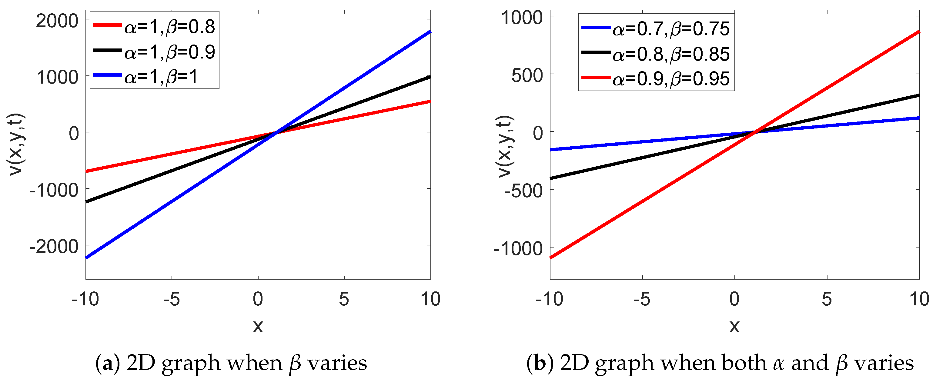
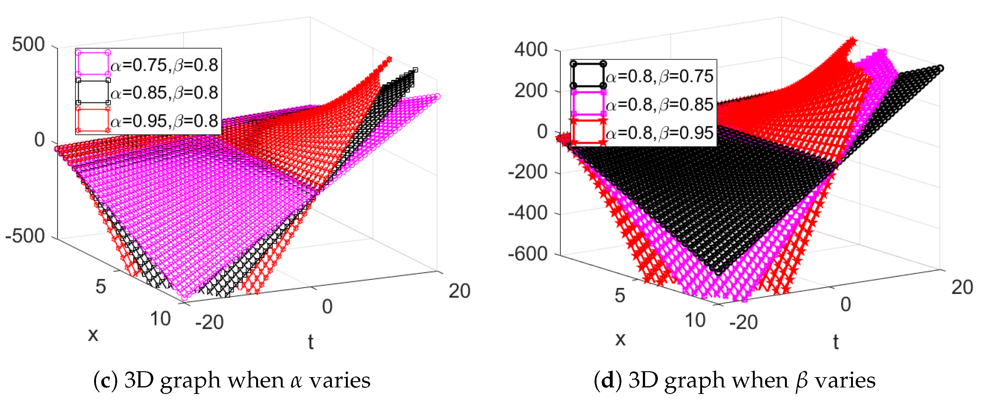
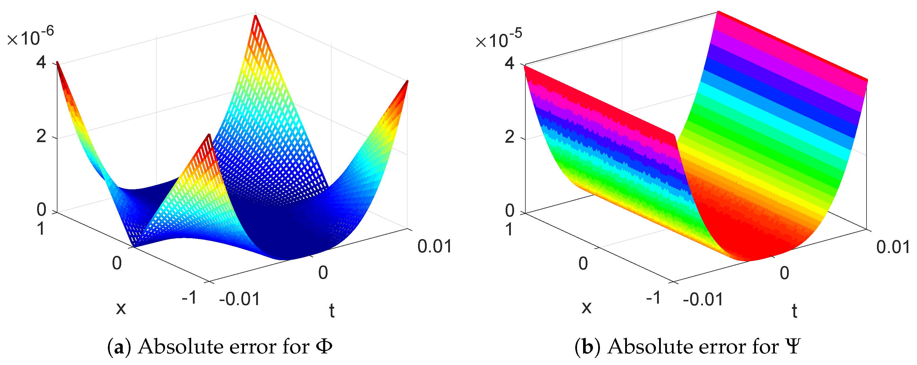
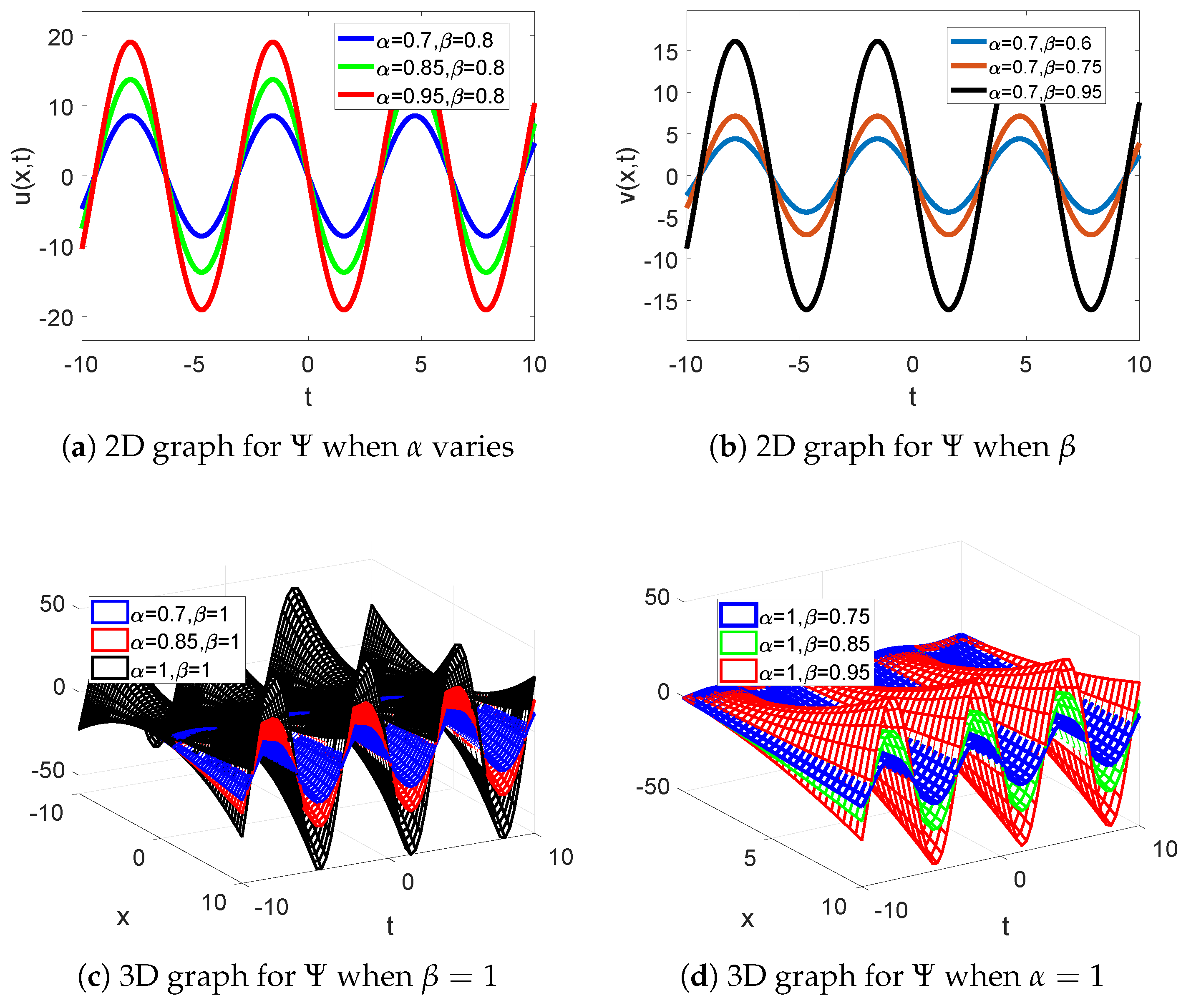
6.1. Simulations and Discussion of Solution of Example 1

In this section, we present the numerical results obtained by applying our proposed method to the nonlinear Burgers equations using the fractal fractional Caputo operator. The numerical simulations were conducted for various values of the fractional order $\alpha$ and the fractal dimension $\beta$. The results are depicted graphically in Figure 1 and Figure 2. In Figure 1a, we observe the two-dimensional behavior of the solution for $\beta$ = 1 and $\alpha$ = 0.8, 0.9, and 0.1. This graph elucidates how the solution evolves for different choices of $\alpha$ while keeping $\beta$ fixed. Next, to portray the effect of the fractal dimension $\beta$, we take $\alpha$ = 1 and vary $\beta$. Figure 1b displays the two-dimensional simulation of the solution for $\beta$ = 0.75, 0.85, and 0.95, while $\alpha$ takes the values 0.7, 0.8, and 0.9. These figures allow us to analyze the impact of $\beta$ on the solution dynamics. To give a more comprehensive analysis, Figure 1c,d portray the three-dimensional behavior of the achieved outcomes for two selected sets of $\alpha$ and $\beta$. These simulations exemplify the complex dynamics of the solution in 3D space and yield further analysis into the system’s behavior. Moreover, Figure 2 represents the two-dimensional and three-dimensional dynamics of the variable $\Psi$ for various combinations of $\alpha$ and $\beta$. These pictures represent the variations in $\Psi$ and how they are affected by the choice of $\alpha$ and $\beta$. From the graphs presented in Figure 1 and Figure 2, it becomes evident that both $\alpha$ and $\beta$ significantly affect the behavior of the obtained results. Even small variations in $\alpha$ or $\beta$ result in notable changes in the solution’s behavior, indicating the sensitivity of the system to these parameters. To explain the accuracy of our technique, we compare the obtained outcomes with the exact solution. Figure 3 studies the absolute error between the series solution and the exact solution. This graph supplies a visual representation of the deviation between the two solutions, allowing us to evaluate the accuracy of our approach. On the top of that,

Table 1. Absolute error between the approximate versus exact solution for $\alpha =1$, $k=1$, $a=1$, $\beta =1$ and $\zeta =0.18$.

($\mathit{\theta }$, t)	$\Phi$	Exact	∣ Exact−$\Phi$ ∣	($\mathit{\theta }$,t)	$\Psi$	Exact	∣ Exact−$\Psi$∣
(−1, 0.01)	9.0218	9.0218	4.3609e−06	(−1, 0.01)	−11.2022	−11.2022	4.0448e−05
(−0.8, 0.01)	9.2178	9.2178	3.5687e−06	(−0.8, 0.01)	−11.0022	−11.0022	4.0440e−05
(−0.6, 0.01)	9.4139	9.4139	2.7766e−06	(−0.6, 0.01)	−10.8021	−10.8021	4.0432e−05
(−0.4, 0.01)	9.6099	9.6099	1.9844e−06	(−0.4, 0.01)	−10.6021	−10.6021	4.0424e−05
(−0.2, 0.01)	9.8060	9.8060	1.1922e−06	(−0.2, 0.01)	−10.4020	−10.4020	4.0416e−05
(0, 0.01)	10.0020	10.0020	4.0008e−07	(0, 0.01)	−10.2020	−10.2020	4.0408e−05
(0.2, 0.01)	10.1980	10.1980	3.9208e−07	(0.2, 0.01)	−10.0020	−10.0020	4.0400e−05
(0.4, 0.01)	10.3941	10.3941	1.1842e−06	(0.4, 0.01)	−9.8019	−9.8020	4.0392e−05
(0.6, 0.01)	10.5901	10.5901	1.9764e−06	(0.6, 0.01)	−9.6019	−9.6019	4.0384e−05
(0.8, 0.01)	10.7862	10.7862	2.7686e−06	(0.8, 0.01)	−9.4018	−9.4019	4.0376e−05
(1, 0.01)	10.9822	10.9822	3.5607e−06	(1, 0.01)	−9.2018	−9.2018	4.0368e−05

presents the numerical values of the absolute error for various parameter values. These values provide quantitative measures of the deviation between the achieved outcomes and the exact solution, further confirming the validity and efficiency of our proposed strategy.

Example 2. 

Consider the 1D-order FF Burgers equation as:

$$\begin{array}{c}\hfill \left\{\begin{array}{c}{}_0^C{D}_{\mathsf{t}}^{\alpha ,\beta }\Phi =2\Phi {\Phi }_{\theta }-{\Phi }_{\theta \theta }+{(\Phi \Psi )}_{\theta },\hfill \\ {}_0^C{D}_{\mathsf{t}}^{\alpha ,\beta }\Psi =-2\Psi {\Psi }_{\theta }-{\Psi }_{\theta \theta }-{(\Phi \Psi )}_{\theta },where0<\alpha ,\beta \le 1,\hfill \end{array}\right.\end{array}$$

(20)

with initial condition $\Phi (\theta ,0)=sin\left(\theta \right)$ , $\Psi (\theta ,0)=-sin\left(\theta \right)$.

Solution 2. 

Since from Equation (20), we have

$$\begin{array}{c}\hfill \left\{\begin{array}{c}{}_0^C{D}_{\mathsf{t}}^{\alpha }\Phi =\beta {\mathsf{t}}^{\beta -1}\left(2\Phi {\Phi }_{\theta }-{\Phi }_{\theta \theta }+{(\Phi \Psi )}_{\theta }\right),\hfill \\ {}_0^C{D}_{\mathsf{t}}^{\alpha }\Psi =\beta {\mathsf{t}}^{\beta -1}\left(-2\Psi {\Psi }_{\theta }-{\Psi }_{\theta \theta }-{(\Phi \Psi )}_{\theta }\right).\hfill \end{array}\right.\end{array}$$

(21)

Applying Natural transform, we obtain

$$\begin{array}{c}\hfill \left\{\begin{array}{c}\frac{S^{\alpha }}{{\rho }^{\alpha }}N\left[\Phi \right]-\frac{S^{\alpha -1}}{{\rho }^{\alpha }}\Phi (\theta ,0)=N\left[\beta {\mathsf{t}}^{\beta -1}\left(2\Phi {\Phi }_{\theta }-{\Phi }_{\theta \theta }+{(\Phi \Psi )}_{\theta }{\Phi }_{\zeta }\right)\right],\hfill \\ \frac{S^{\alpha }}{{\rho }^{\alpha }}N\left[\Psi \right]-\frac{S^{\alpha -1}}{{\rho }^{\alpha }}\Psi (\theta ,0)=N\left[\beta {\mathsf{t}}^{\beta -1}\left(-2\Psi {\Psi }_{\theta }-{\Psi }_{\theta \theta }-{(\Phi \Psi )}_{\theta }\right)\right].\hfill \end{array}\right.\end{array}$$

(22)

$$\begin{array}{c}\hfill \left\{\begin{array}{c}N\left[\Phi \right)=\frac{1}{S}\Phi (\theta ,0)+\frac{{\rho }^{\alpha }}{S^{\alpha }}N\left[\beta {\mathsf{t}}^{\beta -1}\left(2\Phi {\Phi }_{\theta }-{\Phi }_{\theta \theta }+{(\Phi \Psi )}_{\theta }\right)\right],\hfill \\ N\left[\Psi \right]=\frac{1}{S}\Psi (\theta ,0)+\frac{{\rho }^{\alpha }}{S^{\alpha }}N\left[\beta {\mathsf{t}}^{\beta -1}\left(-2\Psi {\Psi }_{\theta }-{\Psi }_{\theta \theta }-{(\Phi \Psi )}_{\theta }\right)\right].\hfill \end{array}\right.\end{array}$$

(23)

Applying the inverse of the Natural transform, we obtain

$$\begin{array}{c}\hfill \left\{\begin{array}{c}\Phi (\theta ,\mathsf{t})=sin\left(\theta \right)+N^{-1}\left[\frac{{\rho }^{\alpha }}{S^{\alpha }}N\left[\beta {\mathsf{t}}^{\beta -1}\left(2\Phi {\Phi }_{\theta }-{\Phi }_{\theta \theta }+{(\Phi \Psi )}_{\theta }\right)\right]\right],\hfill \\ \Psi (\theta ,\mathsf{t})=-sin\left(\theta \right)+N^{-1}\left[\frac{{\rho }^{\alpha }}{S^{\alpha }}N\left[\beta {\mathsf{t}}^{\beta -1}\left(-2\Psi {\Psi }_{\theta }-{\Psi }_{\theta \theta }-{(\Phi \Psi )}_{\theta }\right)\right]\right].\hfill \end{array}\right.\end{array}$$

(24)

The series solution is given by:

$$\begin{array}{c}\hfill \left\{\begin{array}{c}\Phi (\theta ,\mathsf{t})=\sum _{\mathrm{h}=0}^{\infty }{\Phi }_{\mathrm{h}}(\theta ,\mathsf{t},\hfill \\ \Psi (\theta ,\mathsf{t})=\sum _{\mathrm{h}=0}^{\infty }{\Psi }_{\mathrm{h}}(\theta ,\mathsf{t}).\hfill \end{array}\right.\end{array}$$

Now, Equation (24) can be written as:

$$\begin{array}{c}\hfill \left\{\begin{array}{c}\sum _{\mathrm{h}=0}^{\infty }{\Phi }_{\mathrm{h}}(\theta ,\mathsf{t})=sin\left(\theta \right)+N^{-1}\left[\frac{{\rho }^{\alpha }}{S^{\alpha }}N\left[\beta {\mathsf{t}}^{\beta -1}\left(2\sum _{\mathrm{h}=0}^{\infty }{A}_{\mathrm{h}}(\Phi {\Phi }_{\theta })+\sum _{\mathrm{h}=0}^{\infty }{B}_{\mathrm{h}}{(\Phi \Psi )}_{\theta }-\sum _{\mathrm{h}=0}^{\infty }\left({\Phi }_{\theta \theta }\right)\right)\right]\right],\hfill \\ \sum _{\mathrm{h}=0}^{\infty }{\Psi }_{\mathrm{h}}(\theta ,\mathsf{t})=-sin\left(\theta \right)-N^{-1}\left[\frac{{\rho }^{\alpha }}{S^{\alpha }}N\left[\beta {\mathsf{t}}^{\beta -1}\left(2\sum _{\mathrm{h}=0}^{\infty }{C}_{\mathrm{h}}(\Psi {\Psi }_{\theta })+\sum _{\mathrm{h}=0}^{\infty }{D}_{\mathrm{h}}\left({(\Phi \Psi )}_{\theta }\right)+\sum _{\mathrm{h}=0}^{\infty }\left({\Psi }_{\theta \theta }\right)\right)\right]\right].\hfill \end{array}\right.\end{array}$$

where $A_{\mathrm{h}}(\Phi {\Phi }_{\theta })$, $B_{\mathrm{h}}\left({(\Phi \Psi )}_{\theta }\right)$, $C_{\mathrm{h}}(\Psi {\Psi }_{\theta })$, $D_{\mathrm{h}}\left(Phi{\Psi }_{\theta }\right)$ represent Adomian polynomials, which are given below:

$$\begin{array}{c}\hfill \begin{array}{cc}{A}_{\circ }(\Phi {\Phi }_{\theta })={\Phi }_{\circ }{\Phi }_{\circ \theta },\hfill & B_{\circ }\left({(\Phi \Psi )}_{\theta }\right)={\Phi }_{\circ }{\Psi }_{\circ \theta },\hfill \\ A_1(\Phi {\Phi }_{\theta })={\Phi }_{\circ }{\Phi }_{1\theta }+{\Phi }_1{\Phi }_{\circ \theta },\hfill & B_1\left({(\Phi \Psi )}_{\theta }\right)={\Phi }_{\circ \theta }{\Psi }_{1\theta }+{\Phi }_{1\theta }{\Phi }_{\circ \theta },\hfill \\ A_2(\Phi {\Phi }_{\theta })={\Phi }_{\circ }{\Phi }_{2\theta }+{\Phi }_1{\Phi }_{1\theta }+{\Phi }_2{\Phi }_{\circ \theta },\hfill & B_2\left({(\Phi \Psi )}_{\theta }\right)={\Phi }_{\circ \theta }{\Psi }_{2\theta }+{\Phi }_{1\theta }{\Psi }_{1\theta }+{\Phi }_{2\theta }{\Psi }_{\circ \theta },\hfill \\ C_{\circ }(\Psi {\Psi }_{\theta })={\Psi }_{\circ }{\Psi }_{{\circ }_{\theta }},\hfill & D_{\circ }\left({(\Phi \Psi )}_{\theta }\right)={\Phi }_{\circ \theta }{\Psi }_{{\circ }_{\theta }},\hfill \\ C_1(\Psi {\Psi }_{\theta })={\Psi }_{\circ }{\Psi }_{1\zeta }+{\Psi }_1{\Psi }_{\circ \zeta },\hfill & D_1\left({(\Phi \Psi )}_{\theta }\right)={\Phi }_{\circ \theta }{\Psi }_{1\theta }+{\Phi }_{1\theta }{\Psi }_{\circ \theta },\hfill \\ C_2(\Psi {\Psi }_{\theta })={\Psi }_{\circ }{\Psi }_{2\theta }+{\Psi }_1{\Psi }_{1\theta }+{\Psi }_2{\Psi }_{\circ \theta },\hfill & D_2\left({(\Phi \Psi )}_{\theta }\right)={\Phi }_{\circ \theta }{\Psi }_{2\theta }+{\Phi }_{1\theta }{\Psi }_{1\theta }+{\Phi }_{2\theta }{\Psi }_{\circ \theta }.\hfill \end{array}\end{array}$$

Now

$$\begin{array}{c}\hfill \begin{array}{cc}\hfill {\Phi }_{\circ }(\theta ,\mathsf{t})& =sin\left(\theta \right),\hfill \\ \hfill {\Phi }_1(\theta ,\mathsf{t})& =N^{-1}\left[\frac{{\rho }^{\alpha }}{S^{\alpha }}N\left[\beta {\mathsf{t}}^{\beta -1}\left(2A_{\circ }+B_{\circ }+{\Phi }_{\circ \theta \theta }\right)\right]\right]\hfill \\ & =N^{-1}\left[\frac{{\rho }^{\alpha }}{S^{\alpha }}N\left[\beta {\mathsf{t}}^{\beta -1}\left(sin\left(\theta \right)\right)\right]\right]\hfill \\ & =N^{-1}\left[\frac{{\rho }^{\alpha }}{S^{\alpha }}N\left[\beta {\mathsf{t}}^{\beta -1}\left(sin\left(\theta \right)\right)\right]\right]\hfill \\ & =sin\left(\theta \right)\beta N^{-1}\left[\frac{{\rho }^{\alpha }}{S^{\alpha }}\left[(\beta -1)!\frac{{\rho }^{\beta -1}}{S^{\beta }}\right]\right]\hfill \\ & =sin\left(\theta \right)\beta (\beta -1)!N^{-1}\left[\frac{{\rho }^{\alpha +\beta -1}}{S^{\alpha +\beta }}\right]\hfill \\ \hfill {\Phi }_1(\theta ,\mathsf{t})& =\frac{sin\left(\theta \right)\beta (\beta -1)!}{(\alpha +\beta -1)!}{\mathsf{t}}^{\alpha +\beta -1},\hfill \end{array}\end{array}$$

and

$$\begin{array}{c}\hfill {\Phi }_2(\theta ,\mathsf{t})=\frac{sin\left(\theta \right){\beta }^2(\beta -1)!(\alpha +2\beta -2)!}{(\alpha +\beta -1)!(2\alpha +2\beta -2)!}{\mathsf{t}}^{2\alpha +2\beta -2}.\end{array}$$

Similarly

$$\begin{array}{ccc}\hfill {\Psi }_{\circ }(\theta ,\mathsf{t})& =& -sin\left(\theta \right),\hfill \\ \hfill {\Psi }_1(\theta ,\mathsf{t})& =& -\frac{sin\left(\theta \right)\beta (\beta -1)!}{(\alpha +\beta -1)!}{\mathsf{t}}^{\alpha +\beta -1},\hfill \\ \hfill {\Psi }_2(\theta ,\mathsf{t})& =& -\frac{sin\left(\theta \right){\beta }^2(\beta -1)!(\alpha +2\beta -2)!}{(\alpha +\beta -1)!(2\alpha +2\beta -2)!}{\mathsf{t}}^{2\alpha +2\beta -2}.\hfill \end{array}$$

Hence, the required solution is given by

$$\begin{array}{c}\hfill \left\{\begin{array}{c}\Phi (\theta ,\mathsf{t})={\Phi }_{\circ }(\theta ,\mathsf{t})+{\Phi }_1(\theta ,\mathsf{t})+{\Phi }_2(\theta ,\mathsf{t})+\dots \hfill \\ \Psi (\theta ,\mathsf{t})={\Psi }_{\circ }(\theta ,\mathsf{t})+{\Psi }_1(\theta ,\mathsf{t})+{\Psi }_2(\theta ,\mathsf{t})+\dots .\hfill \end{array}\right.\end{array}$$

(25)

$$\begin{array}{ccc}\hfill \Phi (\theta ,\mathsf{t})& =& sin\left(\theta \right)+\frac{sin\left(\theta \right)\beta (\beta -1)!}{(\alpha +\beta -1)!}{\mathsf{t}}^{\alpha +\beta -1}+\frac{sin\left(\theta \right){\beta }^2(\beta -1)!(\alpha +2\beta -2)!}{(2\alpha +2\beta -2)!(\alpha +\beta -1)!}{\mathsf{t}}^{2\alpha +2\beta -2}+\dots ,\hfill \end{array}$$

(26)

$$\begin{array}{ccc}\hfill \Psi (\theta ,\mathsf{t})& =& -sin\left(\theta \right)-\frac{sin\left(\theta \right)\beta (\beta -1)!}{(\alpha +\beta -1)!}{\mathsf{t}}^{\alpha +\beta -1}-\frac{sin\left(\theta \right){\beta }^2(\beta -1)!(\alpha +2\beta -2)!}{(\alpha +\beta -1)!(2\alpha +2\beta -2)!}{\mathsf{t}}^{2\alpha +2\beta -2}-\dots .\hfill \end{array}$$

(27)

Remark 2. 

(a) When $\beta =1$, then

$$\begin{array}{c}\hfill \left\{\begin{array}{c}\Phi (\theta ,\mathsf{t})=sin\left(\theta \right)+\frac{sin\left(\theta \right){\mathsf{t}}^{\alpha }}{\alpha !}+\frac{sin\left(\theta \right)}{\left(2\alpha \right)!}{\mathsf{t}}^{2\alpha }-\dots ,\hfill \\ \Psi (\theta ,\mathsf{t})=-sin\left(\theta \right)-\frac{sin\left(\theta \right){\mathsf{t}}^{\alpha }}{\alpha !}-\frac{sin\left(\theta \right)}{\left(2\alpha \right)!}{\mathsf{t}}^{2\alpha }-\dots ,\hfill \end{array}\right.\end{array}$$

(28)

which is the solution of fractional-order problem given in [27].

(b) 

When $\alpha =\beta =1$ then

$$\begin{array}{c}\hfill \left\{\begin{array}{c}\Phi (\theta ,\mathsf{t})=sin\left(\theta \right)+sin\left(\theta \right)\mathsf{t}+\frac{sin\left(\theta \right)}{2!}{\mathsf{t}}^2+\dots ,\hfill \\ \Psi (\theta ,\mathsf{t})=-sin\left(\theta \right)-sin\left(\theta \right)\mathsf{t}-\frac{sin\left(\theta \right)}{2!}{\mathsf{t}}^2-\dots ,\hfill \end{array}\right.\end{array}$$

the exact solutions are

$$\begin{array}{c}\hfill \left\{\begin{array}{c}\Phi (\theta ,\mathsf{t})=e^{\mathsf{t}}sin\left(\theta \right),\hfill \\ \Psi (\theta ,\mathsf{t})=-e^{\mathsf{t}}sin\left(\theta \right),\hfill \end{array}\right.\end{array}$$

which is the closed-form solution of Equation (20) in integer order.

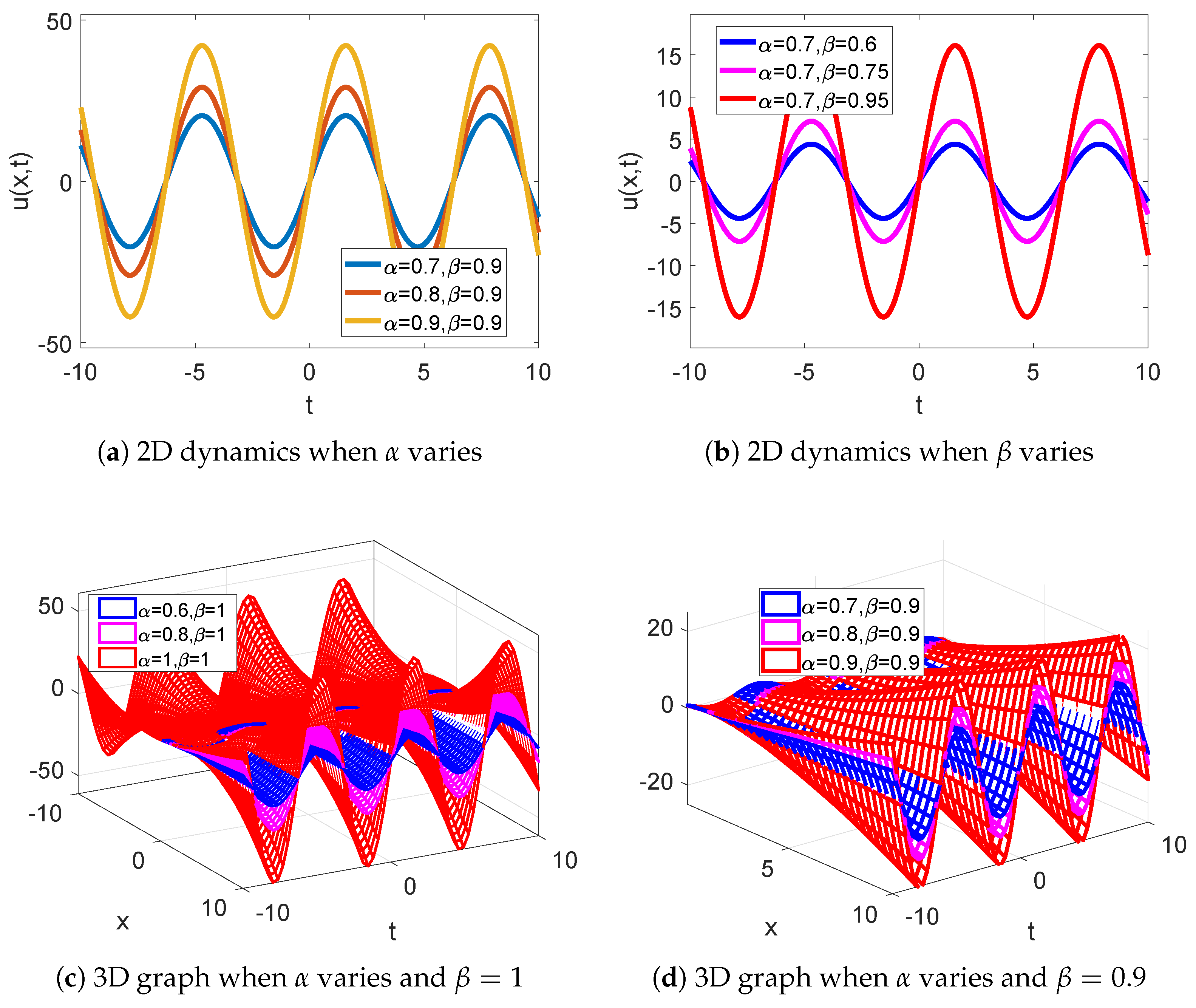
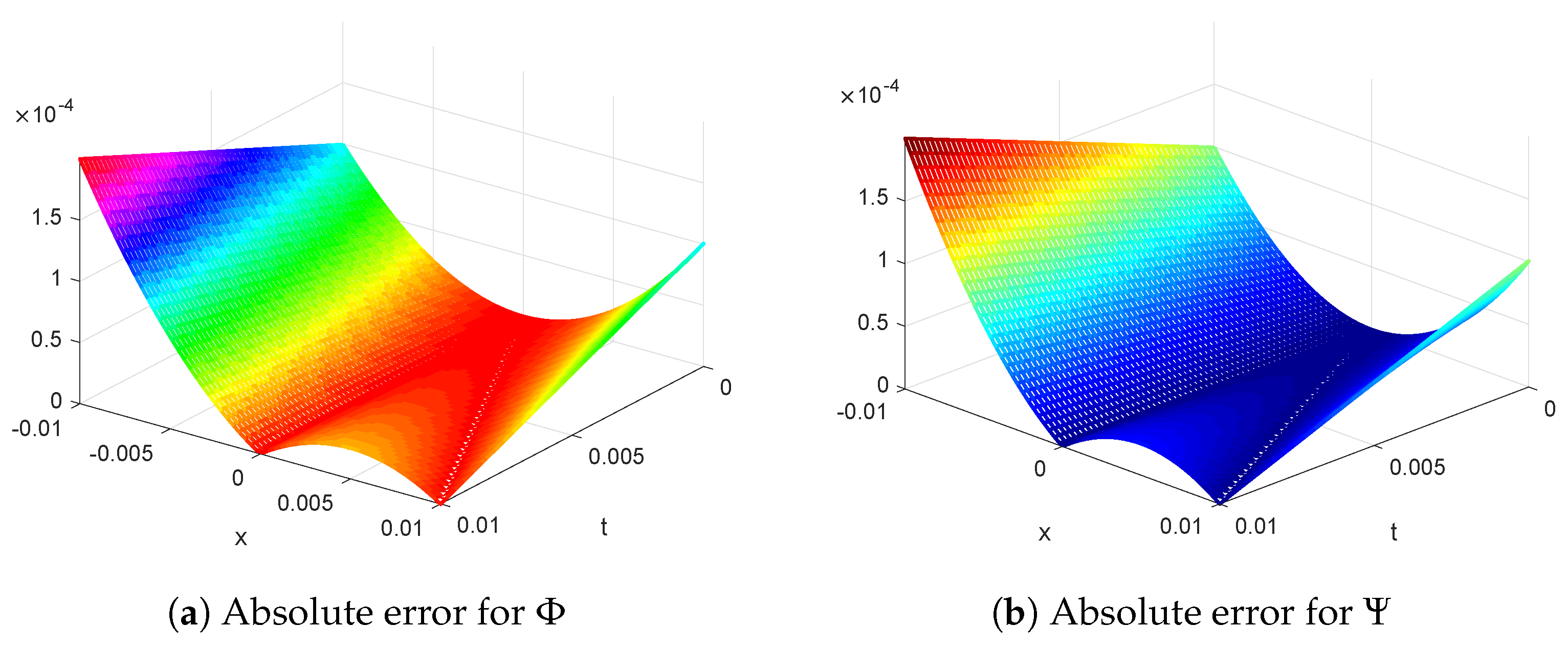
6.2. Simulations and Discussion of Solution of Example 2

In this section, we examine the achieved numerical outcomes for a selection of $\alpha$ and $\beta$. The numerical simulations are graphically represented in Figure 4 and Figure 5, allowing a rigorous and comparative investigation. Figure 4a showcases the two-dimensional behavior of the solution for $\beta$ = 0.9 while varying $\alpha$ between 0.7, 0.8, and 0.9. This plot portrays a detailed investigation of the solution’s evolution under different $\alpha$ values while keeping $\beta$ constant. To further investigate the effect of the fractal dimension $\beta$, we take $\alpha$ = 0.7 and explore varying $\beta$ values. Figure 4b provides a comprehensive two-dimensional simulation of the solution for $\beta$ = 0.6, 0.75, and 0.95, with $\alpha$ fixed at 0.7. These plots help a thorough analysis of how the solution behaves as $\beta$ is adjusted. For a more detailed analysis of the system evolutions, Figure 4c,d display the three-dimensional wave behavior of the obtained outcomes for two specific sets of $\alpha$ and $\beta$. These plots allow valuable insights into the dynamics of the solution in 3D space, enabling a deeper investigation of its behavior. Moreover, Figure 5 gives the 2D and 3D behavior of the variable $\Psi$ across various combinations of $\alpha$ and $\beta$. These graphs represent a comparative assessment of the variations in $\Psi$ and how they are affected by the choice of $\alpha$ and $\beta$. Based on the graphical evaluation presented in Figure 4 and Figure 5, it is noticed that both $\alpha$ and $\beta$ have a great impact on the behavior of the obtained results. Even small variations in $\alpha$ or $\beta$ lead to substantial changes in the solution’s behavior, showing the sensitivity of the system to these parameters. To rigorously analyze the accuracy of our approach, we compare the obtained outcomes with the exact solution. Figure 6 elucidates the absolute error between the acquired series solution and the exact solution, providing a visual representation of the deviation between the two. In addition to that,

Table 2. Absolute error between the approximate versus exact solution for $\alpha =1$, $k=1$, $a=1$, $\beta =1$.

($\mathit{\theta }$, t)	$\Phi$	Exact	∣ Exact−$\Phi$ ∣	($\mathit{\theta }$, t)	$\Psi$	Exact	∣ Exact−$\Psi$∣
(−0.1, 0.01)	−0.0999	−0.0903	9.6e−03	(−0.1, 0.01)	0.0999	0.0903	9.6e−03
(−0.08, 0.01)	−0.0800	−0.0738	6.2e−03	(−0.08, 0.01)	0.0800	0.0738	6.2e−03
(−0.06, 0.01)	−0.0600	−0.0565	3.6e−03	(−0.06, 0.01)	0.0600	0.0565	3.6e−03
(−0.04, 0.01)	−0.0400	−0.0384	1.6e−03	(−0.04, 0.01)	0.0400	0.0384	1.6e−03
(−0.02, 0.01)	−0.0200	−0.0196	4.1601e−04	(−0.02, 0.01)	0.0200	0.0196	4.1601e−04
(0, 0.01)	0	0	0	(0, 0.01)	0	0	0
(0.02, 0.01)	0.0200	0.0204	3.8399e−04	(0.02, 0.01)	−0.0200	−0.0204	3.8399e−04
(0.04, 0.01)	0.0400	0.0416	1.6e−03	(0.04, 0.01)	−0.0400	−0.0416	1.6e−03
(0.06, 0.01)	0.0600	0.0637	3.6e−03	(0.06, 0.01)	−0.0600	−0.0637	3.6e−03
(0.08, 0.01)	0.0800	0.0866	6.6e−03	(0.08, 0.01)	−0.0800	−0.0866	6.6e−03
(0.1, 0.01)	0.0999	0.1103	1.4e−03	(0.1, 0.01)	−0.0999	−0.1103	1.4e−03

gives the numerical values of the absolute error for various parameter combinations, facilitating a quantitative evaluation of the deviation between the achieved outcomes and the exact solution. These comparisons rigorously show the efficiency and validity of our propose method in approximating the exact solution. To sum up, the achieved numerical outcomes presented in this part, as shown in Figure 4 and Figure 5, offer a detailed and comparative study of the solutions obtained by employing the FF Caputo operator in the study of the nonlinear Burgers equations. The graphical representations give insights into the effect of $\alpha$ and $\beta$ on the solution’s evolution, highlighting their significant effect. The analysis of the absolute error portrayed in Figure 6 and Table 2 further proves the efficiency and validity of our technique in approximating the exact solution.

7. Conclusions

The utilization of the FF Caputo operator has been employed to analyze the interconnected nonlinear Burgers equations in a comprehensive manner. In the analysis of differential equations, particularly when nonlocal operators are employed, the theory of existence becomes a pivotal aspect. Consequently, the establishment of existence results, particularly those pertaining to the uniqueness of solutions, has been demonstrated through the aid of functional analysis techniques. Natural transform (NT) offers a generalization of both the Laplace and Sumudu transforms, as can be inferred from the definition of NT itself. Hence, by incorporating NT with Adomian decomposition, the desired solution for the given partial differential equation (PDE) has been derived. The applicability and remarkable accuracy of the applied method have been validated through the examination of Figure 3 and Figure 6 as well as Table 1 and Table 2. Additionally, Figure 7 serves as a visual representation comparing the proposed method with the LADM technique. It is evident from the figure that the proposed method surpasses LADM in terms of efficiency. Moreover, the simulation of the obtained solution effectively illustrates the impact of both the fractional orders $\alpha$ and $\beta$ on the solution of the proposed PDEs. The outcomes of this manuscript offer a more generalized result, as highlighted in Remarks 1 and 2. In the case where $\beta$ equals 1, the solution reduces to the fractional-order case cited in [27]. Furthermore, when both $\alpha$ and $\beta$ assume unity, the solution corresponds to the integer-order case. Thus, the utilization of FF operators for the examination of various equations and models holds significant importance for enhanced analysis.

References

1. Varsoliwala, A.C.; Singh, T.R. Mathematical modeling of atmospheric internal waves phenomenon and its solution by Elzaki Adomian decomposition method. J. Ocean Eng. Sci. 2022, 7, 203–212. [Google Scholar] [CrossRef]
2. Li, Z.; Xia, D.; Cao, J.; Chen, W.; Wang, X. Hydrodynamics study of dolphin’s self-yaw motion realized by spanwise flexibility of caudal fin. J. Ocean Eng. Sci. 2022, 7, 213–224. [Google Scholar] [CrossRef]
3. Jaradat, I.; Alquran, M. A variety of physical structures to the generalized equal-width equation derived from Wazwaz-Benjamin-Bona-Mahony model. J. Ocean Eng. Sci. 2022, 7, 244–247. [Google Scholar] [CrossRef]
4. Fahim, M.R.A.; Kundu, P.R.; Islam, M.E.; Akbar, M.A.; Osman, M.S. Wave profile analysis of a couple of (3 + 1)-dimensional nonlinear evolution equations by sine-Gordon expansion approach. J. Ocean Eng. Sci. 2022, 7, 272–279. [Google Scholar] [CrossRef]
5. Aljahdaly, N.H.; Zobidi, F.O.A. On the Schrödinger equation for deep water waves using the Padé-Adomian decomposition method. J. Ocean Eng. Sci. 2022; in press. [Google Scholar] [CrossRef]
6. Burgers, J.M. A mathematical model illustrating the theory of turbulence. Adv. Appl. Mech. 1948, 1, 171–199. [Google Scholar]
7. Abbasbandy, S.; Darvishi, M.T. A numerical solution of Burgers’ equation by modified Adomian method. Appl. Math. Comput. 2005, 163, 1265–1272. [Google Scholar] [CrossRef]
8. Bahadir, A.R.; Saglam, M. A mixed finite difference and boundary element approach to one-dimensional Burgers’ equation. Appl. Math. Comput. 2005, 160, 663–673. [Google Scholar] [CrossRef]
9. Öziş, T.; Aksan, E.N.; Özdeş, A. A finite element approach for solution of Burgers’ equation. Appl. Math. Comput. 2003, 139, 417–428. [Google Scholar] [CrossRef]
10. Kutluay, S.; Bahadir, A.R.; Özdeş, A. Numerical solution of one-dimensional Burgers’ equation: Explicit and exact-explicit finite difference methods. J. Comput. Appl. Math. 1999, 103, 251–261. [Google Scholar] [CrossRef] [Green Version]
11. Saifullah, S.; Ali, A.; Irfan, M.; Shah, K. Time-Fractional Klein-Gordon Equation with Solitary/Shock Waves Solutions. Math. Probl. Eng. 2021, 2021, 6858592. [Google Scholar] [CrossRef]
12. Ahmad, S.; Ullah, A.; Partohaghighi, M.; Saifullah, S.; Akgül, A.; Jarad, F. Oscillatory and complex behaviour of Caputo-Fabrizio fractional order HIV-1 infection model. AIMS Math. 2022, 7, 4778–4792. [Google Scholar] [CrossRef]
13. Xu, C.; Mu, D.; Liu, Z.; Pang, Y.; Liao, M.; Li, P. Bifurcation dynamics and control mechanism of a fractional-order delayed Brusselator chemical reaction model. MATCH Commun. Math. Comput. 2023, 89, 73–106. [Google Scholar] [CrossRef]
14. Xu, C.; Mu, D.; Liu, Z.; Pang, Y.; Liao, M.; Aouiti, C. New insight into bifurcation of fractional-order 4D neural networks incorporating two different time delays. Commun. Nonlinear Sci. Numer. Simul. 2023, 118, 107043. [Google Scholar] [CrossRef]
15. Ou, W.; Xu, C.; Cui, Q.; Liu, Z.; Pang, Y.; Farman, M.; Ahmad, S.; Zeb, A. Mathematical study on bifurcation dynamics and control mechanism of tri-neuron BAM neural networks including delay. Math. Methods Appl. Sci. 2023. [Google Scholar] [CrossRef]
16. Xu, C.; Zhang, W.; Aouiti, C.; Liu, Z.; Yao, L. Bifurcation insight for a fractional-order stage-structured predator-prey system incorporating mixed time delays. Math. Methods Appl. Sci. 2023, 46, 9103–9118. [Google Scholar] [CrossRef]
17. Xu, C.; Mu, D.; Pan, Y.; Aouiti, C.; Yao, L. Exploring bifurcation in a fractional-order predator-prey system with mixed delays. J. Appl. Anal. Comput. 2022, 13, 1119–1136. [Google Scholar] [CrossRef]
18. Xu, C.; Cui, X.H.; Li, P.L.; Yan, J.L.; Yao, L.Y. Exploration on dynamics in a discrete predator-prey competitive model involving time delays and feedback controls. J. Biol. Dyn. 2023, 17, 2220349. [Google Scholar] [CrossRef] [PubMed]
19. Li, P.L.; Lu, Y.J.; Xu, C.J.; Ren, J. Insight into Hopf bifurcation and control methods in fractional order BAM neural networks incorporating symmetric structure and delay. Cogn. Comput. 2023; in press. [Google Scholar] [CrossRef]
20. Clavin, P. Instabilities and nonlinear patterns of overdriven detonations in gases. In Nonlinear PDE’s in Condensed Matter and Reactive Flows; Springer: Berlin/Heidelberg, Germany, 2002; pp. 49–97. [Google Scholar]
21. Woyczynski, W.A. Lévy processes in the physical sciences. In Lévy Processes; Springer: Berlin/Heidelberg, Germany, 2001; pp. 241–266. [Google Scholar]
22. Sugimoto, N. Burgers equation with a fractional derivative; hereditary effects on nonlinear acoustic waves. J. Fluid Mech. 1991, 225, 631–653. [Google Scholar] [CrossRef]
23. Funaki, T.; Woyczynski, W. Interacting particle approximation for fractal Burgers equation. In Stochastic Processes and Related Topics; Springer: Berlin/Heidelberg, Germany, 1998; pp. 141–166. [Google Scholar]
24. Aljahdaly, N.H.; Agarwal, R.P.; Shah, R.; Botmart, T. Analysis of the Time Fractional-Order Coupled Burgers Equations with Non-Singular Kernel Operators. Mathematics 2021, 9, 2326. [Google Scholar] [CrossRef]
25. Shah, N.A.; El-Zahar, E.R.; Chung, J.D. Fractional Analysis of Coupled Burgers Equations within Yang Caputo-Fabrizio Operator. J. Funct. Spaces 2022, 2022, 6231921. [Google Scholar] [CrossRef]
26. Mao, Z.; Karniadakis, G.E. Fractional Burgers equation with nonlinear non-locality: Spectral vanishing viscosity and local discontinuous Galerkin methods. J. Comput. Phys. 2017, 336, 143–163. [Google Scholar] [CrossRef]
27. Khan, H.; Kumam, P.; Khan, Q.; Khan, S.; Hajira; Arshad, M.; Sitthithakerngkiet, K. The Solution Comparison of Time-Fractional Non-Linear Dynamical Systems by Using Different Techniques. Front. Phys. 2022, 10, 863551. [Google Scholar] [CrossRef]
28. Saifullah, S.; Ali, A.; Shah, K.; Promsakon, C. Investigation of Fractal Fractional nonlinear Drinfeld–Sokolov–Wilson system with Non-singular Operators. Results Phys. 2022, 33, 105145. [Google Scholar] [CrossRef]
29. Gulalai; Ullah, A.; Ahmad, S.; Inc, M. Fractal fractional analysis of modified KdV equation under three different kernels. J. Ocean Eng. Sci. 2022; in press. [Google Scholar]
30. Xuan, L.; Ahmad, S.; Ullah, A.; Saifullah, S.; Akgül, A.; Qu, H. Bifurcations, stability analysis and complex dynamics of Caputo fractal-fractional cancer model. Chaos Solitons Fract. 2022, 159, 112113. [Google Scholar] [CrossRef]
31. Saifullah, S.; Ali, A.; Goufo, E.F.D. Investigation of complex behaviour of fractal fractional chaotic attractor with Mittag-Leffler Kernel. Chaos Solitons Fract. 2021, 152, 111332. [Google Scholar] [CrossRef]
32. Alqahtani, R.T.; Ahmad, S.; Akgül, A. On Numerical Analysis of Bio-Ethanol Production Model with the Effect of Recycling and Death Rates under Fractal Fractional Operators with Three Different Kernels. Mathematics 2022, 10, 1102. [Google Scholar] [CrossRef]
33. Atangana, A. Fractal-fractional differentiation and integration: Connecting fractal calculus and fractional calculus to predict complex system. Chaos Solitons Fract. 2017, 102, 396–406. [Google Scholar] [CrossRef]
34. Khan, Z.H.; Khan, W.A. N-transform properties and applications. NUST J. Eng. Sci. 2008, 1, 127–133. [Google Scholar]
35. Loonker, D.; Banerji, P.K. Solution of fractional ordinary differential equations by natural transform. Int. J. Math. Eng. Sci. 2013, 12, 1–7. [Google Scholar]
36. Khamsi, M. Remarks on Cone Metric Spaces and Fixed Point Theorems of Contractive Mappings. Fixed Point Theory Appl. 2010, 2010, 315398. [Google Scholar] [CrossRef] [Green Version]
37. Guo, D.; Lakshmikantham, V. Coupled fixed foints of nonlinear Operators with applications. Nonlinear Anal. Theory Methods Appl. 1987, 11, 623–632. [Google Scholar] [CrossRef]
Figure 1. Simulations of the solution of Equation (12) for various sets of  α  and  β u ( x , t )  denotes the  Φ ( θ , ζ , t )  in the above figures.
Fractalfract 07 00551 g001
Figure 2. Simulations of the solution v(x, y, t) of Equation (12) for various sets of  α  and  β . Here, v(x, y, t) represents  Ψ ( θ , ζ , t )  in the above figures.
Fractalfract 07 00551 g002aFractalfract 07 00551 g002b
Figure 3. Simulation of the absolute error.
Fractalfract 07 00551 g003
Figure 4. Simulations of the solution of Equation (20) for various sets of  α  and  β .
Fractalfract 07 00551 g004
Figure 5. Simulations of the solution of the Equation (20) for various sets of  α  and  β .
Fractalfract 07 00551 g005
Figure 6. Simulation of the absolute error.
Fractalfract 07 00551 g006
Figure 7. Comparison of the proposed approach with Laplace Adomian decomposition method (LADM).
Fractalfract 07 00551 g007