New Results on $\mathbf{(}\mathit{r}\mathbf{,}\mathit{k}\mathbf{,}\mathit{\mu }\mathbf{)}$-Riemann–Liouville Fractional Operators in Complex Domain with Applications

Abstract

This paper introduces fractional operators in the complex domain as generalizations for the Srivastava–Owa operators. Some properties for the above operators are also provided. We discuss the convexity and starlikeness of the generalized Libera integral operator. A condition for the convexity and starlikeness of the solutions of fractional differential equations is provided. Finally, a fractional differential equation is converted into an ordinary differential equation by wave transformation; illustrative examples are provided to clarify the solution within the complex domain.

1. Introduction and Definitions

Fractional calculus theory has found interesting applications in analytic function theory. The standard definitions of fractional operators and their extensions have been effectively utilized to derive various results, such as characterization properties, coefficient estimates [1], and distortion inequalities [2].

The complex modeling of phenomena in nature and society has recently been the object of several investigations based on methods initially developed in a physical context. These systems are the consequence of the ability of individuals to develop strategies. They occur in complex dynamical systems [3], kinetic theory [4], and hyperchaotic complex systems [5]. Fractional differential equations concerning the Riemann-Liouville fractional operators or the Caputo derivative have been recommended by many authors (see [6,7,8,9,10,11]).

In Section 1, we introduce generalizations for the Srivastava-Owa fractional operators. The conditions for the boundedness of the fractional integral operator in Bergman space are provided. Additionally, certain features are also given for these operators. In Section 2, we generalize the Libera integral operator [12], and we discuss the convexity and starlikeness for this operator. Additionally, results are presented for some fractional differential equations that have convex (starlike) solutions. In Section 3, the generalization of the wave transformation is introduced. This transformation converts differential equations in the complex domain from fractional into ordinary, with illustrative examples.

In [13], Srivastava and Owa presented the definitions of fractional operators in the complex domain as follows:

Definition 1.

The fractional integral of order $\alpha$ is given for an analytic function$f$in a simple connected region of a complex plane by

$$I_z^{\delta }f\left(z\right)=\frac{1}{\Gamma \left(\delta \right)}\underset{0}{\overset{z}{\int }}f\left(v\right) {(z-v)}^{\delta -1} dv ; \delta >0.$$

Definition 2.

The fractional derivative of order $\delta$ is defined for an analytic function $f$ in a simple connected region of a complex plane as

$$\begin{array}{ll}{D}_z^{\delta }f\left(z\right)& =\frac{1}{\Gamma (1-\delta )} \frac{d}{dz}\underset{0}{\overset{z}{\int }}\frac{f\left(v\right)}{{(z-v)}^{\delta }} dv ; 0\le \delta <1\\ & =\frac{d}{dz}{I}_z^{1-\delta } f\left(z\right).\end{array}$$

Remark 1.

From Definitions 1 and 2, we have the following:

(1)

$D_z^{\delta }{z}^{\beta }=\frac{\mathrm{\Gamma }\left(\beta +1\right)}{\mathrm{\Gamma }\left(\beta -\delta +1\right)}{z}^{\beta -\delta },\beta >-1;0\le \delta <1$.

(2)

$I_z^{\delta }{z}^{\beta }=\frac{\mathrm{\Gamma }\left(\beta +1\right)}{\mathrm{\Gamma }\left(\beta +\delta +1\right)}{z}^{\beta +\delta },\beta >-1;0\le \delta <1$.

We recall some definitions that can be found in [14]. Let $\mathcal{H}$ denote the class of analytic functions in the open unit disk $U=\left\{z:\left|z\right|<1\right\}$. For $n\in {\mathbb{Z}}^{+}$ and $a\in \mathbb{C}$, let

$$\mathcal{H}\left[a,n\right]=\left\{f\in \mathcal{H}:f\left(z\right)=a+a_n{z}^n+a_{n+1}{z}^{n+1}+\cdots \right\}.$$

Let the class $\mathcal{A}\subseteq \mathcal{H}\left[\mathrm{0,1}\right]$ be defined as follows:

$$\mathcal{A}=\{f\in \mathcal{H}:f\left(z\right)=z+{\sum }_{n=2}^{\infty }{a}_n{z}^n\}.$$

The subclass $\mathcal{S}$ of $\mathcal{A}$ consists of univalent functions (the functions that are one-to-one and analytic in $U$). A function $f\in \mathcal{A}$ is said to be starlike (convex, resp.) of order $\rho$ (where $0\le \rho <1$) if it satisfies $Re\left(\frac{z{f}^{\prime }\left(z\right)}{f\left(z\right)}\right)>\rho$ ($Re(\frac{z{f}^{″}\left(z\right)}{f^{\prime }\left(z\right)}+1)>\rho$, resp.).

2. $\mathbf{(}\mathit{r}\mathbf{,}\mathit{k}\mathbf{,}\mathit{\mu }\mathbf{)}$-Riemann–Liouville Fractional Operators

To begin, we generalize the definitions of gamma functions given in [5,14] as follows:

Definition 3.

For $\delta \in \mathbb{C},Re\left(\delta \right)>1-\frac{1}{r}, r\in \mathbb{N},\mathrm{and} k>0$, the $\left(r,k\right)$-gamma function ${\Gamma }_{r,k}$ is defined as follows (see Figure 1):

$${\Gamma }_{r,k}\left(\delta \right)={\int }_0^{\infty }{t}^{r(\delta -1)} e^{-\frac{t^k}{k}} dt$$

(1)

Remark 2.

In the above definition, the following hold:

(1)

If we take $r=k=1$, then ${\mathrm{\Gamma }}_{r,k}\left(\delta \right)=\mathrm{\Gamma }\left(\delta \right)$.

(2)

If we take $r=1$, we obtain the $k–$gamma function’s definition in [5].

(3)

If we take $k=1$, then ${\mathrm{\Gamma }}_{r,k}\left(\delta \right)={\mathrm{\Gamma }}_{t^r}\left(\delta \right)$ in [14].

Proposition 1.

Suppose $k>0, r\in \mathbb{N},\mathrm{and} \delta$ and $\beta$ in $\mathbb{C}$ with $Re\left(\delta \right)>1-\frac{1}{r}, Re\left(\beta \right)>1-\frac{1}{r}$. Then, the following hold:

(1)

${\mathrm{\Gamma }}_{r,k}\left(\frac{k+r-1}{r}\right)=1$.

(2)

${\mathrm{\Gamma }}_{r,k}\left(\delta \right)=k^{\frac{r\left(\delta -1\right)+1-k}{k}} \mathrm{\Gamma }\left(\frac{r\left(\delta -1\right)+1}{k}\right)$.

(3)

${\mathrm{\Gamma }}_{r,k}\left(\delta \right)={\Gamma }_k\left(r\left(\delta -1\right)+1\right)$.

(4)

${\mathrm{\Gamma }}_{r,k}\left(\delta +\frac{k}{r}\right)=\left(r\left(\delta -1\right)+1\right){\mathrm{\Gamma }}_{r,k}\left(\delta \right)$.

Proof.  

From the above definition and direct calculations. □

In the following definitions and results, we present fractional operators in terms of the $\left(r,k\right)–$gamma function.

Definition 4.

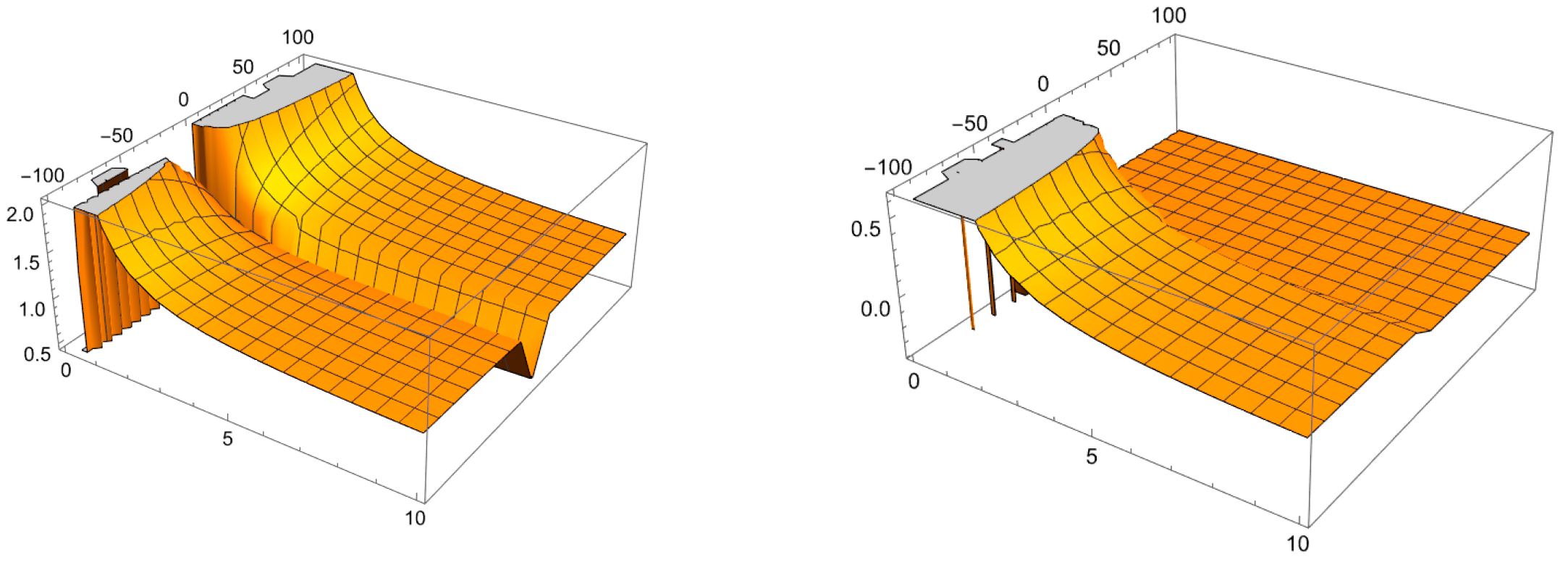
Let $f$ be a continuous function in $\overline{U}$. Then, the $\left(r,k,\mu \right)$-Riemann-Liouville fractional integral is defined as follows (see Figure 2):

$$I_{(r,k,\mu )}^{\delta } f\left(z\right)=\frac{{(\mu +1)}^{1-\frac{r\left(\delta -1\right)+1}{k}}}{k {\Gamma }_{r,k}\left(\delta \right)}{\int }_0^z{(z^{\mu +1}-v^{\mu +1})}^{\frac{r\left(\delta -1\right)+1}{k}-1} v^{\mu } f\left(v\right) dv$$

(2)

where $\in \mathbb{N},k>0, \delta \ge 1-\frac{1}{r}$, and $\mu \ge 0$.

Figure 2. Plots of $\mathrm{R}\mathrm{e}\left({\mathrm{I}}_{\left(3,\mathrm{k},0\right)}^{0.75}1\right)$, $\mathrm{I}\mathrm{m}\left({\mathrm{I}}_{\left(3,\mathrm{k},0\right)}^{0.75}1\right)$, $\mathrm{R}\mathrm{e}\left({\mathrm{I}}_{\left(3,\mathrm{k},0\right)}^{0.75}\mathrm{z}\right)$, and $\mathrm{I}\mathrm{m}\left({\mathrm{I}}_{\left(3,\mathrm{k},0\right)}^{0.75}\mathrm{z}\right)$.

Figure 2. Plots of $\mathrm{R}\mathrm{e}\left({\mathrm{I}}_{\left(3,\mathrm{k},0\right)}^{0.75}1\right)$, $\mathrm{I}\mathrm{m}\left({\mathrm{I}}_{\left(3,\mathrm{k},0\right)}^{0.75}1\right)$, $\mathrm{R}\mathrm{e}\left({\mathrm{I}}_{\left(3,\mathrm{k},0\right)}^{0.75}\mathrm{z}\right)$, and $\mathrm{I}\mathrm{m}\left({\mathrm{I}}_{\left(3,\mathrm{k},0\right)}^{0.75}\mathrm{z}\right)$.

Definition 5.

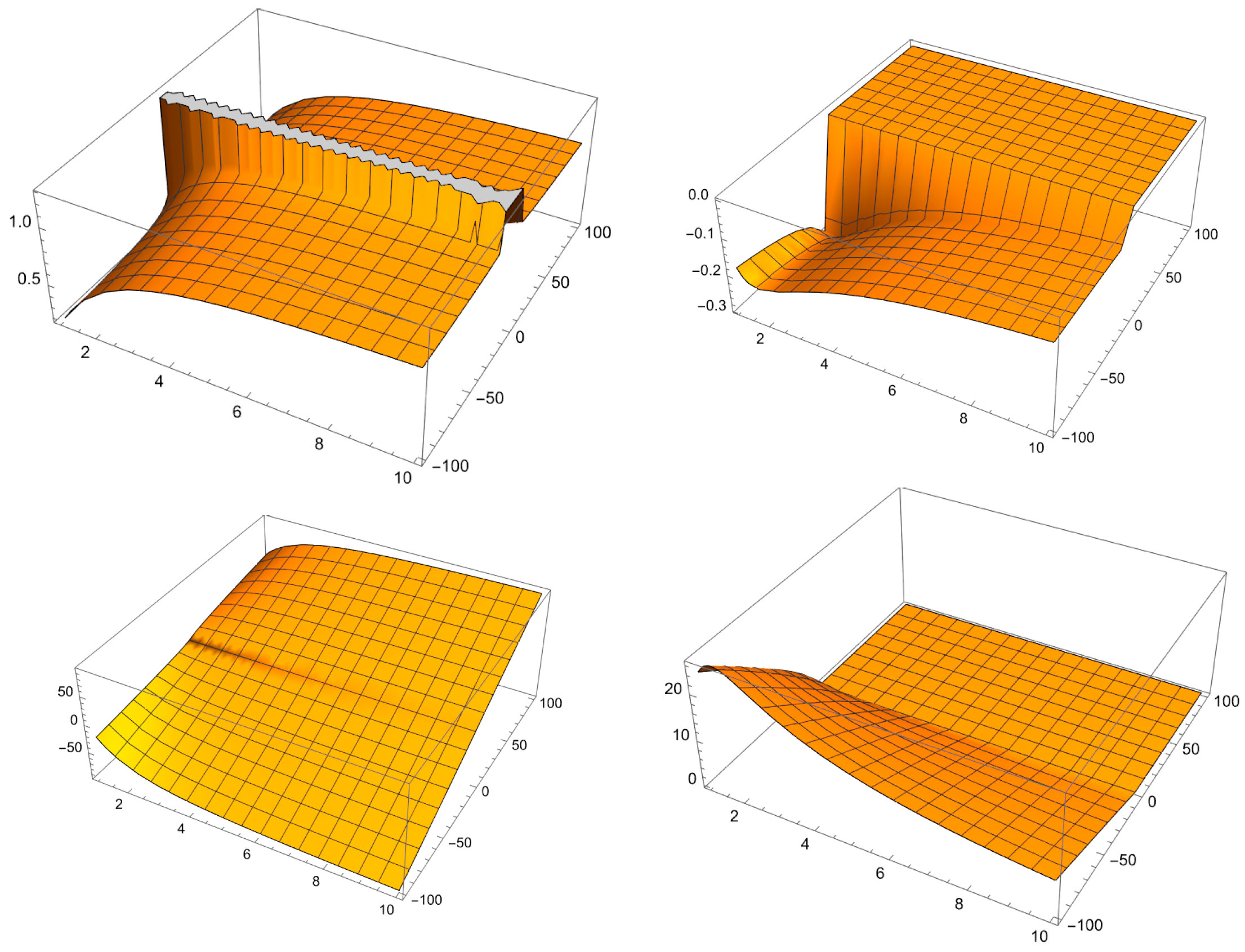
Let $f\in C^n\left(\overline{U}\right), n=\left[\frac{r\left(\delta -1\right)+1}{k}\right]+1, r\in \mathbb{N},k>0,$ and $\delta \in \mathbb{R}$. Then, the $\left(r,k,\mu \right)$-Riemann-Liouville fractional derivative is defined as follows (see Figure 3):

$$\begin{array}{ll}{D}_{(r,k,\mu )}^{\delta } f\left(z\right)& ={\left(\frac{d}{dz}\right)}^n\frac{{(\mu +1)}^{1-n+\frac{r\left(\delta -1\right)+1}{k}}{k}^{n-1}}{ {\Gamma }_{r,k}\left(\frac{nk-2}{r}-(\delta -2)\right) }{\int }_0^z{(z^{\mu +1}-v^{\mu +1})}^{n-\frac{r\left(\delta -1\right)+1}{k}-1} v^{\mu } f\left(v\right) dv\\ & ={\left(\frac{d}{dz}\right)}^n\frac{{(\mu +1)}^{1-n+\frac{r\left(\delta -1\right)+1}{k}}{k}^{n-1}}{ {\Gamma }_k\left(nk-(r\left(\delta -1\right)+1)\right) }{\int }_0^z{(z^{\mu +1}-v^{\mu +1})}^{n-\frac{r\left(\delta -1\right)+1}{k}-1} v^{\mu } f\left(v\right) dv\\ & ={\left(\frac{d}{dz}\right)}^n{k}^n{I}_{(r,k,\mu )}^{\frac{nk-2}{r}-(\delta -2)} f(z)\end{array}$$

(3)

Figure 3. Plots of $\mathrm{R}\mathrm{e}\left({\mathrm{D}}_{\left(3,\mathrm{k},0\right)}^{0.75}1\right)$, $\mathrm{I}\mathrm{m}\left({\mathrm{D}}_{\left(3,\mathrm{k},0\right)}^{0.75}1\right)$, $\mathrm{R}\mathrm{e}\left({\mathrm{D}}_{\left(3,\mathrm{k},0\right)}^{0.75}\mathrm{z}\right)$, and $\mathrm{I}\mathrm{m}\left({\mathrm{D}}_{\left(3,\mathrm{k},0\right)}^{0.75}\mathrm{z}\right)$.

Figure 3. Plots of $\mathrm{R}\mathrm{e}\left({\mathrm{D}}_{\left(3,\mathrm{k},0\right)}^{0.75}1\right)$, $\mathrm{I}\mathrm{m}\left({\mathrm{D}}_{\left(3,\mathrm{k},0\right)}^{0.75}1\right)$, $\mathrm{R}\mathrm{e}\left({\mathrm{D}}_{\left(3,\mathrm{k},0\right)}^{0.75}\mathrm{z}\right)$, and $\mathrm{I}\mathrm{m}\left({\mathrm{D}}_{\left(3,\mathrm{k},0\right)}^{0.75}\mathrm{z}\right)$.

Remark 3.

In Definitions 4 and 5, the following hold:

(1)

If $\mu =0$ and $r=k=1$, we obtain Srivastava and Owa’s definitions in [13].

(2)

If $r=k=1$, then we obtain the definitions by Ibrahim in [15].

(3)

If $\mu =0$ and $r=1$, then we obtain the definitions by Ibrahim in [16].

Proposition 2.

For $\delta ,\beta >0$, the following statements hold:

(1)

$I_{(r,k,\mu )}^{\delta }{I}_{(r,k,\mu )}^{\beta }f\left(z\right)=I_{(r,k,\mu )}^{(\delta +\beta -1+\frac{1}{r})}f(z)$.

(2)

$I_{(r,k,\mu )}^{\delta }$and $D_{(r,k,\mu )}^{\delta }$ are linear operators.

(3)

$I_{(r,k,\mu )}^{\delta } z^{\beta }=\frac{{(\mu +1)}^{-\frac{r\left(\delta -1\right)+1}{k}} \Gamma \left(\frac{\beta }{\mu +1}+1\right)}{k^{\frac{r\left(\delta -1\right)+1}{k}} \Gamma \left(\frac{r\left(\delta -1\right)+1}{k}+1+\frac{\beta }{\mu +1}\right)} z^{\frac{r\left(\delta -1\right)+1}{k}\left(\mu +1\right)+\beta }, \beta >-(\mu +1)$

(4)

$D_{(r,k,\mu )}^{\delta } z^{\beta }=\frac{{(\mu +1)}^{\frac{r\left(\delta -1\right)+1}{k}} \Gamma \left(\frac{\beta }{\mu +1}+1\right)}{k^{-\frac{r\left(\delta -1\right)+1}{k}} \Gamma \left(\frac{\beta }{\mu +1}-\frac{r\left(\delta -1\right)+1}{k}+1\right)} z^{\left(\mu +1\right)\left(1-\frac{r\left(\delta -1\right)+1}{k}\right)+\beta -1}, 0\le \frac{r\left(\delta -1\right)+1}{k}<1, \beta >-(\mu +1)$

(5)

$D_{\left(r,k,\mu \right)}^{\delta } I_{\left(r,k,\mu \right)}^{\delta } z^{\beta }=z^{\mu +\beta }, 0\le \frac{r\left(\delta -1\right)+1}{k}<1$

(6)

If $f$ is analytic, then $D_{\left(r,k,\mu \right)}^{\delta }{I}_{\left(r,k,\mu \right)}^{\delta }f\left(z\right)=z^{\mu }f\left(z\right),0\le \frac{r\left(\delta -1\right)+1}{k}<1$.

(7)

If $0\le \frac{r\left(\delta -1\right)+1}{k}<1$ and $0\le \frac{r\left(\beta -1\right)+1}{k}<1$, then $D_{\left(r,k,\mu \right)}^{\delta }{I}_{\left(r,k,\mu \right)}^{\beta }f\left(z\right)=\left\{\begin{array}{l}{z}^{\mu }{I}_{\left(r,k,\mu \right)}^{\left(\beta -\delta +1-\frac{1}{r}\right)} f\left(z\right), \beta >\delta \\ D_{\left(r,k,\mu \right)}^{\left(\delta -\beta +1-\frac{1}{r}\right)} f\left(z\right), \delta >\beta .\end{array}\right.$

(8)

$D_{\left(r,k,0\right)}^{\delta }{I}_{\left(r,k,0\right)}^{\delta }f\left(z\right)=f\left(z\right),n=\left[\frac{\delta }{k}\right]+1$.

(9)

If $\delta \ge \beta$, $n=\left[\frac{\delta }{k}\right]+1$, and $m=\left[\frac{\beta }{k}\right]+1$, then

$$I_{(1,k,0)}^{\delta }{D}_{(1,k,0)}^{\beta }f\left(z\right)=I_{(1,k,0)}^{\delta -\beta }f\left(z\right)-{\sum }_{j=1}^m\frac{z^{\frac{\delta }{k}-j}}{k{\mathrm{\Gamma }}_k\left(\delta +\left(1-j\right)k\right)}{D}_{\left(1,k,0\right)}^{\beta -jk}f(0).$$

(10)

If $\delta +\beta <nk$, $n=\left[\frac{\delta }{k}\right]+1$, and $m=\left[\frac{\beta }{k}\right]+1$, then

$$D_{(1,k,0)}^{\delta }{D}_{(1,k,0)}^{\beta }f\left(z\right)=D_{(1,k,0)}^{\delta +\beta }f\left(z\right)-{\sum }_{j=1}^m\frac{z^{-\frac{\delta }{k}-j}}{k^{-j+1-\frac{\delta }{k}}\mathrm{\Gamma }\left(1-\frac{\delta }{k}-j\right)}{D}_{\left(1,k,0\right)}^{\beta -jk}f(0).$$

Proof.  

(1)

$$\begin{gathered} I_{(r,k,\mu )}^{\delta }{I}_{(r,k,\mu )}^{\beta } f\left(z\right)=\frac{{(\mu +1)}^{1-\frac{r\left(\delta -1\right)+1}{k}}}{k {\mathrm{\Gamma }}_{r,k}\left(\delta \right)}{\int }_0^z{(z^{\mu +1}-v^{\mu +1})}^{\frac{r\left(\delta -1\right)+1}{k}-1} v^{\mu } I_{(r,k,\mu )}^{\beta } f\left(v\right) dv \\ =\frac{{(\mu +1)}^{2-\frac{r\left(\delta +\beta -2\right)+2}{k}}}{k^2 {\mathrm{\Gamma }}_{r,k}\left(\delta \right){\mathrm{\Gamma }}_{r,k}\left(\beta \right)}{\int }_0^z{\left(z^{\mu +1}-v^{\mu +1}\right)}^{\frac{r\left(\delta -1\right)+1}{k}-1} v^{\mu } ({\int }_0^v{\left(v^{\mu +1}-w^{\mu +1}\right)}^{\frac{r\left(\beta -1\right)+1}{k}-1} w^{\mu } f\left(w\right) dw ) dv \\ =\frac{{(\mu +1)}^{2-\frac{r\left(\left(\delta +\beta -1+\frac{1}{r}\right)-1\right)+1}{k}}}{k^2{\mathrm{\Gamma }}_{r,k}\left(\delta \right){\mathrm{\Gamma }}_{r,k}\left(\beta \right)}{\int }_0^z{w}^{\mu }f\left(w\right)({\int }_w^z{\left(z^{\mu +1}-v^{\mu +1}\right)}^{\frac{r\left(\delta -1\right)+1}{k}-1}{v}^{\mu }{ \left(v^{\mu +1}-w^{\mu +1}\right)}^{\frac{r\left(\beta -1\right)+1}{k}-1}dv)dw \end{gathered}$$

(by Dirichlet equality).

Substituting $x=(v^{\mu +1}-w^{\mu +1})/(z^{\mu +1}-w^{\mu +1})$ into the above integration yields

$$\begin{array}{l}{I}_{(r,k,\mu )}^{\delta }{I}_{(r,k,\mu )}^{\beta }f\left(z\right)=\frac{{(\mu +1)}^{2-\frac{r\left(\left(\delta +\beta -1+\frac{1}{r}\right)-1\right)+1}{k}}}{k^2{\mathrm{\Gamma }}_{r,k}\left(\delta \right){\mathrm{\Gamma }}_{r,k}\left(\beta \right)}{\int }_0^z{w}^{\mu }f(w)\frac{{(z^{\mu +1}-w^{\mu +1})}^{\frac{r\left\{\left(\delta +\beta -1+\frac{1}{r}\right)-1\right\}+1}{k}-1}}{(\mu +1)}\\ \left({\int }_0^1{(1-x)}^{\frac{r\left(\delta -1\right)+1}{k}-1}{x}^{\frac{r\left(\beta -1\right)+1}{k}-1}dx\right)dw\\ =\frac{{(\mu +1)}^{1-\frac{r\left(\left(\delta +\beta -1+\frac{1}{r}\right)-1\right)+1}{k}}}{k^2{\mathrm{\Gamma }}_{r,k}\left(\delta \right){\mathrm{\Gamma }}_{r,k}\left(\beta \right)}B\left(\frac{r\left(\delta -1\right)+1}{k},\frac{r\left(\beta -1\right)+1}{k}\right){\int }_0^z{w}^{\mu }f(w){(z^{\mu +1}-w^{\mu +1})}^{\frac{r\left\{\left(\delta +\beta -1+\frac{1}{r}\right)-1\right\}+1}{k}-1}dw\\ =\frac{{(\mu +1)}^{1-\frac{r\left(\left(\delta +\beta -1+\frac{1}{r}\right)-1\right)+1}{k}}}{k{\mathrm{\Gamma }}_{r,k}\left(\delta +\beta -1+\frac{1}{r}\right)}{\int }_0^z{w}^{\mu }f(w){(z^{\mu +1}-w^{\mu +1})}^{\frac{r\left\{\left(\delta +\beta -1+\frac{1}{r}\right)-1\right\}+1}{k}-1}dw\\ =I_{\left(r,k,\mu \right)}^{\left(\delta +\beta -1+\frac{1}{r}\right)}f(z).\end{array}$$

(2)

Clear.

(3)

$I_{(r,k,\mu )}^{\delta }{z}^{\beta }=\frac{{(\mu +1)}^{1-\frac{r\left(\delta -1\right)+1}{k}}}{k{\mathrm{\Gamma }}_{r,k}\left(\delta \right)}{\int }_0^z{(z^{\mu +1}-v^{\mu +1})}^{\frac{r\left(\delta -1\right)+1}{k}-1}{v}^{\mu +\beta }dv$

Set $y={\left(\frac{v}{z}\right)}^{\mu +1}$; then, $z{y}^{\frac{1}{\mu +1}}=v$ and, hence,

$$\begin{array}{ll}{I}_{\left(r,k,\mu \right)}^{\delta }{z}^{\beta }& =\frac{{\left(\mu +1\right)}^{-\frac{r\left(\delta -1\right)+1}{k}}}{k{\mathrm{\Gamma }}_{r,k}\left(\delta \right)}{\int }_0^1{z}^{\left(\mu +1\right)\left\{\frac{r\left(\delta -1\right)+1}{k}-1\right\}}{\left(1-y\right)}^{\frac{r\left(\delta -1\right)+1}{k}-1}{z}^{\mu +\beta +1}{y}^{\frac{\beta }{\mu +1}}dy\\ & =\frac{{\left(\mu +1\right)}^{-\frac{r\left(\delta -1\right)+1}{k}}}{k{\mathrm{\Gamma }}_{r,k}\left(\delta \right)}{z}^{\frac{r\left(\delta -1\right)+1}{k}\left(\mu +1\right)+\beta }\frac{\mathrm{\Gamma }\left(\frac{r\left(\delta -1\right)+1}{k}\right)\mathrm{\Gamma }\left(\frac{\beta +\mu +1}{\mu +1}\right)}{\mathrm{\Gamma }\left(\frac{r\left(\delta -1\right)+1}{k}+\frac{\beta +\mu +1}{\mu +1}\right)}\\ & =\frac{{\left(\mu +1\right)}^{-\frac{r\left(\delta -1\right)+1}{k}}\mathrm{\Gamma }\left(\frac{\beta +\mu +1}{\mu +1}\right)}{k^{\frac{r\left(\delta -1\right)+1}{k}}\mathrm{\Gamma }\left(\frac{r\left(\delta -1\right)+1}{k}+\frac{\beta +\mu +1}{\mu +1}\right)}{z}^{\frac{r\left(\delta -1\right)+1}{k}\left(\mu +1\right)+\beta }\end{array}$$

(4)

$D_{(r,k,\mu )}^{\delta }{z}^{\beta }=\frac{d}{dz}\frac{{(\mu +1)}^{\frac{r\left(\delta -1\right)+1}{k}}}{{\mathrm{\Gamma }}_k\left(k-\left(r\left(\delta -1\right)+1\right)\right)}{\int }_0^z{(z^{\mu +1}-v^{\mu +1})}^{-\frac{r\left(\delta -1\right)+1}{k}}{v}^{\mu +\beta }dv$

Set $={\left(\frac{v}{z}\right)}^{\mu +1}$; then, $z{y}^{\frac{1}{\mu +1}}=v$, yielding

$$\begin{array}{ll}{D}_{(r,k,\mu )}^{\delta }{z}^{\beta }& =\frac{d}{dz}\frac{{(\mu +1)}^{\frac{r\left(\delta -1\right)+1}{k}-1}}{{\mathrm{\Gamma }}_{r,k}\left(\left(\frac{k-2}{r}\right)-\left(\delta -2\right)\right)}{\int }_0^z{z}^{\left(\mu +1\right)\left(-\frac{r\left(\delta -1\right)+1}{k}\right)}{(1-y)}^{-\frac{r\left(\delta -1\right)+1}{k}}{z}^{\mu +\beta +1}{y}^{\frac{\beta }{\mu +1}}dy\\ & =\frac{d}{dz}\frac{{(\mu +1)}^{\frac{r\left(\delta -1\right)+1}{k}-1}}{k^{-\frac{r\left(\delta -1\right)+1}{k}} \mathrm{\Gamma }\left(1-\frac{r\left(\delta -1\right)+1}{k}\right)}{z}^{\left(\mu +1\right)\left(1-\frac{r\left(\delta -1\right)+1}{k}\right)+\beta }\frac{\mathrm{\Gamma }\left(1-\frac{r\left(\delta -1\right)+1}{k}\right)\mathrm{\Gamma }\left(\frac{\beta }{\mu +1}+1\right)}{\mathrm{\Gamma }\left(\frac{\beta }{\mu +1}+2-\frac{r\left(\delta -1\right)+1}{k}\right)}\\ & =\frac{{(\mu +1)}^{\frac{r\left(\delta -1\right)+1}{k}}\mathrm{\Gamma }\left(\frac{\beta }{\mu +1}+1\right)}{k^{-\frac{r\left(\delta -1\right)+1}{k}}\mathrm{\Gamma }\left(\frac{\beta }{\mu +1}-\frac{r\left(\delta -1\right)+1}{k}+1\right)}{z}^{\left(\mu +1\right)\left(1-\frac{r\left(\delta -1\right)+1}{k}\right)+\beta -1}\end{array}$$

(5)

Follows from (3) and (4).

(6)

Follows from (5).

(7)

If $\beta >\delta$, then

$$\begin{array}{ll}{D}_{\left(r,k,\mu \right)}^{\delta }{I}_{\left(r,k,\mu \right)}^{\beta }f\left(z\right)& =D_{\left(r,k,\mu \right)}^{\delta }\left(I_{\left(r,k,\mu \right)}^{\delta }{I}_{\left(r,k,\mu \right)}^{\beta -\delta +1-\frac{1}{r}}f\left(z\right)\right), \mathrm{by} (1)\\ & =D_{\left(r,k,\mu \right)}^{\delta }{I}_{\left(r,k,\mu \right)}^{\delta }\left(I_{\left(r,k,\mu \right)}^{\beta -\delta +1-\frac{1}{r}}f\left(z\right)\right), \mathrm{by} (6)\\ & =z^{\mu }{I}_{\left(r,k,\mu \right)}^{\beta -\delta +1-\frac{1}{r}}f\left(z\right).\end{array}$$

If $\delta >\beta$, then

$$\begin{array}{ll}{D}_{\left(r,k,\mu \right)}^{\delta }{I}_{\left(r,k,\mu \right)}^{\beta }f\left(z\right)& =\frac{d}{dz}k{I}_{\left(r,k,\mu \right)}^{\frac{k-2}{r}-\left(\delta -2\right)}\left(I_{\left(r,k,\mu \right)}^{\beta }f\left(z\right)\right)\\ & =\frac{d}{dz}k{I}_{\left(r,k,\mu \right)}^{\frac{k-2}{r}-\left(\delta -2\right)+\beta -1+\frac{1}{r}}f\left(z\right)\\ & =\frac{d}{dz}k{I}_{\left(r,k,\mu \right)}^{\frac{k-2}{r}-\left(\left(\delta -\beta +1-\frac{1}{r}\right)-2\right)}f(z)\\ & =D_{\left(r,k,\mu \right)}^{\delta -\beta +1-\frac{1}{r}}f(z).\end{array}$$

(8)

$\begin{array}{ll}{D}_{\left(r,k,0\right)}^{\delta }{I}_{\left(r,k,0\right)}^{\delta }f\left(z\right)& ={\left(\frac{d}{dz}\right)}^n{k}^n{I}_{\left(r,k,0\right)}^{\frac{nk-2}{r}-\left(\delta -2\right)}\left(I_{\left(r,k,0\right)}^{\delta }f\left(z\right)\right)\\ & ={\left(\frac{d}{dz}\right)}^n{k}^n{I}_{\left(r,k,0\right)}^{\frac{nk-2}{r}-\left(\delta -2\right)+\delta -1+\frac{1}{r}}f(z)\\ & ={\left(\frac{d}{dz}\right)}^n{k}^n{I}_{\left(r,k,0\right)}^{\frac{nk-1}{r}+1}f(z)\\ & ={\left(\frac{d}{dz}\right)}^n{k}^n\left\{\frac{1}{k{\mathrm{\Gamma }}_k\left(nk\right)}{\int }_0^z{\left(z-v\right)}^{n-1}f\left(v\right)dv\right\}\\ & =f\left(z\right).\end{array}$

(9)

$\begin{array}{ll}{I}_{\left(1,k,0\right)}^{\delta }{D}_{\left(1,k,0\right)}^{\beta }f\left(z\right)& =\frac{1}{k{\mathrm{\Gamma }}_k\left(\delta \right)}{\int }_0^z{(z-v)}^{\frac{\delta }{k}-1}{D}_{\left(1,k,0\right)}^{\beta }f\left(v\right)dv\\ & =\frac{d}{dz}\left\{\frac{1}{\alpha {\mathrm{\Gamma }}_k\left(\delta \right)}{\int }_0^z{\left(z-v\right)}^{\frac{\delta }{k}}{D}_{\left(1,k,0\right)}^{\beta }f\left(v\right)dv\right\}\\ & =\frac{d}{dz}\left\{\frac{1}{k^{\frac{\delta }{k}}\mathrm{\Gamma }\left(\frac{\delta }{k}-n+1\right)}{\int }_0^z{\left(z-v\right)}^{\frac{\delta }{k}-n}{k}^n{I}_{\left(1,k,0\right)}^{nk-\beta }f\left(v\right)dv-\sum _{j=1}^m\frac{z^{\frac{\delta }{k}-j+1}}{k^{\frac{\delta }{k}}\mathrm{\Gamma }\left(\frac{\delta }{k}-j+2\right)}{\left(\frac{d}{dz}\right)}^{n-j}{k}^n{I}_{\left(1,k,0\right)}^{nk-\beta }f\left(0\right)\right\}\\ & =\frac{d}{dz}\left\{k{I}_{\left(1,k,0\right)}^{\delta -nk+k}{I}_{\left(1,k,0\right)}^{nk-\beta }f(z)-\sum _{j=1}^m\frac{z^{\frac{\delta }{k}-j+1}}{k^{\frac{\delta }{k}}\mathrm{\Gamma }\left(\left(\frac{\delta -jk}{k}+1\right)+1\right)}{\left(\frac{d}{dz}\right)}^{n-j}{k}^n{I}_{\left(1,k,0\right)}^{nk-\beta }f\left(0\right)\right\}\\ & =\frac{d}{dz}\left\{k{I}_{\left(1,k,0\right)}^{k+(\delta -\beta )}f(z)-\sum _{j=1}^m\frac{k^{j-1}{z}^{\frac{\delta -jk}{k}+1}}{k^{\frac{\delta }{k}-1}\mathrm{\Gamma }\left(\left(\frac{\delta -jk}{k}+1\right)+1\right)}{D}_{\left(1,k,0\right)}^{\beta -jk}f\left(0\right)\right\}\\ & =I_{\left(1,k,0\right)}^{(\delta -\beta )}f(z)-\sum _{j=1}^m\frac{z^{\frac{\delta }{k}-j}}{k{\mathrm{\Gamma }}_k\left(\delta -jk+k\right)}{D}_{\left(1,k,0\right)}^{\beta -jk}f(0)\end{array}$

(10)

$\begin{array}{ll}{D}_{(1,k,0)}^{\delta }{D}_{(1,k,0)}^{\beta }f\left(z\right)& ={\left(\frac{d}{dz}\right)}^n{k}^n{I}_{\left(1,k,0\right)}^{nk-\delta }\left(D_{\left(1,k,0\right)}^{\beta }f\left(z\right)\right)\\ & ={\left(\frac{d}{dz}\right)}^n{k}^n\left\{I_{\left(1,k,0\right)}^{\left(nk-\delta -\beta \right)}f\left(z\right)-\sum _{j=1}^m\frac{z^{\frac{nk-\delta }{k}-j}}{k{\mathrm{\Gamma }}_k\left(nk-\delta +k-jk\right)}{D}_{\left(1,k,0\right)}^{\beta -jk}f\left(0\right)\right\}\\ & ={\left(\frac{d}{dz}\right)}^{n+m}{k}^{n+m}{I}_{\left(1,k,0\right)}^{\left((n+m)k-\left(\delta +\beta \right)\right)}f\left(z\right)-\sum _{j=1}^m\left({\left(\frac{d}{dz}\right)}^n{k}^n\frac{z^{n-\frac{\delta }{k}-j}}{k^{n-j+1-\frac{\delta }{k}}\mathrm{\Gamma }\left(n-\frac{\delta }{k}-j+1\right)}\right)D_{\left(1,k,0\right)}^{\beta -jk}f\left(0\right)\\ & =D_{\left(1,k,0\right)}^{\delta +\beta }f\left(z\right)-\sum _{j=1}^m\left(\frac{z^{-\frac{\delta }{k}-j}}{k^{-j+1-\frac{\delta }{k}}\mathrm{\Gamma }\left(1-\frac{\delta }{k}-j\right)}\right)D_{\left(1,k,0\right)}^{\beta -jk}f\left(0\right)\end{array}$

□

Example 1.

Consider the fractional differential equation $D_{\left(\mathrm{1,3},0\right)}^{\frac{3}{2}}u\left(z\right)=u\left(z\right)$ with $D_{\left(\mathrm{1,3},0\right)}^{-\frac{3}{2}}u\left(0\right)=-2\sqrt{\frac{\pi }{3}}$; then,

$$\begin{array}{ll}{D}_{\left(\mathrm{1,3},0\right)}^{\frac{3}{2}}\left(D_{\left(\mathrm{1,3},0\right)}^{\frac{3}{2}}u\left(z\right)\right)& =D_{\left(\mathrm{1,3},0\right)}^{3}u\left(z\right)-\frac{z^{-\frac{3}{2}} \sqrt{3}}{\Gamma \left(-\frac{1}{2}\right)}{D}_{\left(\mathrm{1,3},0\right)}^{-\frac{3}{2}}u\left(0\right)\\ & ={\left(\frac{d}{dz}\right)}^2{3}^2{I}_{\left(\mathrm{1,3},0\right)}^{2\left(3\right)-3}u\left(z\right)-z^{-\frac{3}{2}}\\ & =3\frac{d}{dz}\left\{\frac{d}{dz}3 I_{\left(\mathrm{1,3},0\right)}^{3}u\left(z\right)\right\}-z^{-\frac{3}{2}}\\ & =3u^{\prime }\left(z\right)-z^{-\frac{3}{2}}.\end{array}$$

Additionally,

$$D_{\left(\mathrm{1,3},0\right)}^{\frac{3}{2}}\left(D_{\left(\mathrm{1,3},0\right)}^{\frac{3}{2}}u\left(z\right)\right)=D_{\left(\mathrm{1,3},0\right)}^{\frac{3}{2}}u\left(z\right)=u\left(z\right).$$

Consequently,

$$3u^{\prime }\left(z\right)-z^{-\frac{3}{2}}=u\left(z\right).$$

Therefore,

$$u\left(z\right)e^{-\frac{z}{3}}={\int }_0^z\frac{1}{3}{w}^{-\frac{3}{2}}{e}^{-w}dw.$$

Recall that for $\mathrm{p}\in {\mathbb{R}}^{+},$the Bergman space ${\mathrm{A}}^{\mathrm{p}}$ is the class of all analytic functions $\mathrm{f}$ in $\mathrm{U}$ with ${‖\mathrm{f}‖}_{{\mathrm{A}}^{\mathrm{p}}}^{\mathrm{p}}<\infty$, where the norm is defined by

$${‖f‖}_{A^p}={\left(\frac{1}{\pi }{\int }_U{\left|f\left(z\right)\right|}^{p}d\sigma \right)}^{\frac{1}{p}},z\in U,$$

(4)

where $d\sigma$ denotes the Lebesgue area measure. In the following theorem, it is shown that the integral operator is bounded in $A^p$.

Theorem 1. 

Let $0<p<\infty , \delta >1-\frac{1}{r}, k>0, r\in \mathbb{N},$ and $\mu \ge 0$. Then, $I_{(r,k,\mu )}^{\delta }$ is bounded in $A^p$ and

$${‖I_{\left(r,k,\mu \right)}^{\delta }f\left(z\right)‖}_{A^P}^p\le C{‖f\left(z\right)‖}_{A^p}^p,$$

where

$$C≔{\int }_0^1{\left|\frac{{\left(\mu +1\right)}^{1-\frac{r\left(\delta -1\right)+1}{k}}}{k{\mathrm{\Gamma }}_{r,k}\left(\delta \right)}\left({\left(1-w^{\mu +1}\right)}^{\frac{r\left(\delta -1\right)+1}{k}-1}{w}^{\mu }\right)dw\right|}^p.$$

Proof.  

Assume that $f\in A^P$. Then,

$$\begin{array}{l}{‖I_{\left(r,k,\mu \right)}^{\delta }f\left(z\right)‖}_{A^P}^p=\frac{1}{\pi }{\int }_U{\left|I_{\left(r,k,\mu \right)}^{\delta }f\left(z\right)\right|}^{p}d\sigma \\ =\frac{1}{\pi }{\int }_0^1{\left|\frac{{(\mu +1)}^{1-\frac{r\left(\delta -1\right)+1}{k}}}{k{\mathrm{\Gamma }}_{r,k}\left(\delta \right)}{\int }_0^z{\left(z^{\mu +1}-v^{\mu +1}\right)}^{\frac{r\left(\delta -1\right)+1}{k}-1}{v}^{\mu }f(v)dv\right|}^{p}d\sigma \\ =\frac{1}{\pi }{\int }_0^1{\left|\frac{{(\mu +1)}^{1-\frac{r\left(\delta -1\right)+1}{k}}}{k{\mathrm{\Gamma }}_{r,k}\left(\delta \right)}{\int }_0^1{\left(1-w^{\mu +1}\right)}^{\frac{r\left(\delta -1\right)+1}{k}-1}{z}^{\left(\mu +1\right)\left(\frac{r\left(\delta -1\right)+1}{k}\right)}{w}^{\mu }f(wz)dw\right|}^{p}d\sigma \\ \le \frac{1}{\pi }{\int }_0^1{\left|\frac{{(\mu +1)}^{1-\frac{r\left(\delta -1\right)+1}{k}}}{k{\mathrm{\Gamma }}_{r,k}\left(\delta \right)}{\int }_U{\left(1-w^{\mu +1}\right)}^{\frac{r\left(\delta -1\right)+1}{k}-1}{w}^{\mu }f(wz)dw\right|}^{p}d\sigma \\ \le {\int }_0^1{\left|\frac{{\left(\mu +1\right)}^{1-\frac{r\left(\delta -1\right)+1}{k}}}{k{\mathrm{\Gamma }}_{r,k}\left(\delta \right)}{\int }_U{\left(1-w^{\mu +1}\right)}^{\frac{r\left(\delta -1\right)+1}{k}-1}{w}^{\mu }dw\right|}^p\left(\frac{1}{\pi }{\int }_U{\left|f\left(v\right)\right|}^{p}dA\right)≔C{‖f‖}_{A^p}^p\end{array}$$

where $w=\frac{v}{z}$. □

Definition 6.

Let $f\in C^n\left(\overline{U}\right),\mu \ge 0,k>0, r\in \mathbb{N},\delta \ge 1-\frac{1}{r}, \mathrm{and} n=\left[\frac{r\left(\delta -1\right)+1}{k}\right]+1$. Then, the $(r,k,\mu )$-Caputo derivative is defined by

$$c{D}_{\left(r,k,\mu \right)}^{\delta }f(z)=k^n{I}_{(r,k,\mu )}^{\frac{nk-2}{r}-(\delta -2)} f^{\left(n\right)}(z)$$

(5)

Theorem 2.

Let $\delta >1-\frac{1}{r}, r\in \mathbb{N},n=\left[\frac{r\left(\delta -1\right)+1}{k}\right]+1$, and $f$ be an analytic function. Then,

$$D_{\left(r,k,0\right)}^{\delta }f\left(z\right)={\sum }_{j=0}^{n-1}\frac{z^{j-\frac{r\left(\delta -1\right)+1}{k}} f^{\left(j\right)}\left(0\right)}{k^{-\frac{r\left(\delta -1\right)+1}{k}} \Gamma \left(j+1-\frac{r\left(\delta -1\right)+1}{k}\right)}+c{D}_{\left(r,k,\mu \right)}^{\delta }f(z)$$

(6)

Proof.  

We have

$$f\left(z\right)=\sum _{j=0}^{n-1}\frac{z^j}{\Gamma \left(j+1\right)} f^{\left(j\right)}\left(0\right)+R_{n-1},$$

where

$$\begin{array}{ll}{R}_{n-1}& ={\int }_0^z\frac{f^{\left(n\right)}\left(y\right){(z-y)}^{n-1}}{\left(n-1\right)!}dy\\ & =\frac{1}{\mathrm{\Gamma }\left(n\right)}{\int }_0^z{f}^{\left(n\right)}\left(y\right){(z-y)}^{n-1}dy\\ & =\frac{k^n}{k{k}^{\frac{kn}{k}-1}\Gamma (n)}{\int }_0^z{f}^{\left(n\right)}\left(y\right){(z-y)}^{\frac{kn}{k}-1}dy\\ & =\frac{k^n}{k{\mathrm{\Gamma }}_k\left(r\left\{\left(\frac{nk-1}{r}+1\right)-1\right\}+1\right)}{\int }_0^z{f}^{\left(n\right)}\left(y\right){(z-y)}^{\frac{r\left(\left\{\frac{nk-1}{r}+1\right\}-1\right)+1}{k}-1}dy\\ & =k^n{I}_{(r,k,0)}^{\frac{nk-1}{r}+1}{f}^{\left(n\right)}(z)\end{array}$$

(7)

Thus,

$$\begin{array}{ll}{D}_{\left(r,k,0\right)}^{\delta }f\left(z\right)& =\sum _{j=0}^{n-1}\frac{D_{(r,k,0)}^{\delta }{z}^j}{\mathrm{\Gamma }\left(j+1\right)}{f}^{\left(j\right)}\left(0\right)+D_{(r,k,0)}^{\delta }{R}_{n-1}\\ & =\sum _{j=0}^{n-1}\frac{z^{j-\frac{r\left(\delta -1\right)+1}{k}}{f}^{\left(j\right)}\left(0\right)}{k^{-\frac{r\left(\delta -1\right)+1}{k}}\mathrm{\Gamma }\left(j+1-\frac{r\left(\delta -1\right)+1}{k}\right)}+D_{\left(r,k,0\right)}^{\delta }{k}^n{I}_{\left(r,k,0\right)}^{\frac{nk-1}{r}+1}{f}^{\left(n\right)}(z)\\ & =\sum _{j=0}^{n-1}\frac{z^{j-\frac{r\left(\delta -1\right)+1}{k}}{f}^{\left(j\right)}\left(0\right)}{k^{-\frac{r\left(\delta -1\right)+1}{k}}\mathrm{\Gamma }\left(j+1-\frac{r\left(\delta -1\right)+1}{k}\right)}+k^n{I}_{\left(r,k,0\right)}^{\left(\frac{nk-1}{r}+1\right)-\delta +1-\frac{1}{r}}{f}^{\left(n\right)}(z)\\ & =\sum _{j=0}^{n-1}\frac{z^{j-\frac{r\left(\delta -1\right)+1}{k}}{f}^{\left(j\right)}\left(0\right)}{k^{-\frac{r\left(\delta -1\right)+1}{k}}\mathrm{\Gamma }\left(j+1-\frac{r\left(\delta -1\right)+1}{k}\right)}+k^n{I}_{\left(r,k,0\right)}^{\frac{nk-2}{r}-(\delta -2)}{f}^{\left(n\right)}(z)\\ & =\sum _{j=0}^{n-1}\frac{z^{j-\frac{r\left(\delta -1\right)+1}{k}}{f}^{\left(j\right)}\left(0\right)}{k^{-\frac{r\left(\delta -1\right)+1}{k}}\mathrm{\Gamma }\left(j+1-\frac{r\left(\delta -1\right)+1}{k}\right)}+c{D}_{\left(r,k,0\right)}^{\delta }f(z).\end{array}$$

□

3. Convexity and Starlikeness

In this section, we generalize the Libera integral operator (see [12]) using an operator of the form

$${\mathcal{F}}_{\left(r,k,\delta \right)}\left(z\right)=\frac{k^{\frac{r\left(\delta -1\right)+1}{k}}\mathrm{\Gamma }\left(\frac{r\left(\delta -1\right)+1}{k}+2\right)}{z^{\frac{r\left(\delta -1\right)+1}{k}}}{I}_{\left(r,k,0\right)}^{\delta }f(z)$$

(8)

or, equivalently,

$${\mathcal{F}}_{\left(r,k,\delta \right)}\left(z\right)=\frac{\left(\frac{r\left(\delta -1\right)+1}{k}\right)\left(\frac{r\left(\delta -1\right)+1}{k}+1\right)}{z^{\frac{r\left(\delta -1\right)+1}{k}}}{\int }_0^z{(z-\nu )}^{\frac{r\left(\delta -1\right)+1}{k}-1}f\left(\nu \right)d\nu$$

(9)

Recall that the class of admissible functions ${\mathsf{\Psi }}_n\{\mathsf{\Omega },1\}$ consists of those functions $\mathsf{\psi }:{\mathbb{C}}^3\times U⟶\mathbb{C}$ that satisfy the admissibility condition (see [17]):

$$\begin{gathered} \psi (\rho i,\sigma ,\mu +\nu i;z)\notin \mathsf{\Omega }\hspace{1em}\mathrm{when}\hspace{1em}\rho ,\sigma ,\mu ,\nu \in \mathbb{R}\hspace{1em}\mathrm{and}\hspace{1em}\mathsf{\Omega }\subseteq \mathbb{C} \\ \sigma \le -\frac{n}{2}\left(1+{\rho }^2\right),\sigma +\mu \le 0,z\in U \end{gathered}$$

(10)

Theorem 3

([17]). Let $p\in \mathcal{A}$. If $\psi \in {\Psi }_n\{\Omega ,1\}$ and $\psi \left(p\left(z\right),z{p}^{\prime }\left(z\right), z^2{p}^{″}\left(z\right);z\right)\in \Omega$, then $Re\left(p\left(z\right)\right)>0$.

Theorem 4.

Let $f\in \mathcal{A}$ and $\delta \ge \frac{k-1}{r}+1$

$$Re\left(\frac{z{\mathcal{F}}_{\left(r,k,\delta -\frac{k}{r}\right)}^{\prime }\left(z\right)}{{\mathcal{F}}_{\left(r,k,\delta -\frac{k}{r}\right)}\left(z\right)}\right)>-\frac{1}{2}.$$

Then, ${\mathcal{F}}_{\left(r,k,\delta \right)}\left(z\right)$ is a starlike function.

Proof.  

Let $\left(z\right)=\frac{z{\mathcal{F}}_{\left(r,k,\delta -\frac{k}{r}\right)}^{\prime }\left(z\right)}{{\mathcal{F}}_{\left(r,k,\delta -\frac{k}{r}\right)}\left(z\right)}$. Then, $p$ is analytic and $p\left(0\right)=1$. Hence,

$$\begin{gathered} {\mathcal{F}}_{\left(r,k,\delta \right)}^{\prime }\left(z\right)=\frac{\left(\frac{r\left(\delta -1\right)+1}{k}\right)\left(\frac{r\left(\delta -1\right)+1}{k}+1\right)}{z^{\frac{r\left(\delta -1\right)+1}{k}}}{\int }_0^z\left(\frac{r\left(\delta -1\right)+1}{k}-1\right){\left(z-\nu \right)}^{\frac{r\left(\delta -1\right)+1}{k}-2}f\left(\nu \right)d\nu - \\ \frac{{\left(\frac{r\left(\delta -1\right)+1}{k}\right)}^2\left(\frac{r\left(\delta -1\right)+1}{k}+1\right)}{z^{\frac{r\left(\delta -1\right)+1}{k}+1}}{\int }_0^z{(z-\nu )}^{\frac{r\left(\delta -1\right)+1}{k}-1}f\left(\nu \right)d\nu . \end{gathered}$$

This implies that

$$z{\mathcal{F}}_{\left(r,k,\delta \right)}^{\prime }\left(z\right)=\left(\frac{r\left(\delta -1\right)+1}{k}+1\right){\mathcal{F}}_{\left(r,k,\delta -\frac{k}{r}\right)}\left(z\right)-\left(\frac{r\left(\delta -1\right)+1}{k}\right){\mathcal{F}}_{\left(r,k,\delta \right)}\left(z\right).$$

Consequently,

$${\mathcal{F}}_{\left(r,k,\delta \right)}\left(z\right)\left\{p\left(z\right)+\left(\frac{r\left(\delta -1\right)+1}{k}\right)\right\}=\left(\frac{r\left(\delta -1\right)+1}{k}+1\right){\mathcal{F}}_{\left(r,k,\delta -\frac{k}{r}\right)}\left(z\right).$$

We then obtain

$$\frac{z{\mathcal{F}}_{\left(r,k,\delta -\frac{k}{r}\right)}^{\prime }\left(z\right)}{{\mathcal{F}}_{\left(r,k,\delta -\frac{k}{r}\right)}\left(z\right)}=\frac{z{p}^{\prime }\left(z\right)}{p\left(z\right)+\left(\frac{r\left(\delta -1\right)+1}{k}\right)}+p\left(z\right)=\psi \left(p\left(z\right),z{p}^{\prime }\left(z\right);z\right),$$

which leads to $Re\left(\psi \left(p\left(z\right),z{p}^{\prime }\left(z\right);z\right)\right)>-\frac{1}{2}$. The admissibility condition $\psi \in {\mathsf{\Psi }}_1\left\{\mathsf{\Omega },1\right\}$ is satisfied as follows:

$$Re\left(\rho i+\frac{\sigma }{\rho i+\left(\frac{r\left(\delta -1\right)+1}{k}\right)}\right)=\frac{\sigma }{{\rho }^2+{\left(\frac{r\left(\delta -1\right)+1}{k}\right)}^2}\le -\frac{1}{2}.$$

Thus, $Re\left(p\left(z\right)\right)>0$ and ${\mathcal{F}}_{(r,k,\delta )}$ is starlike. □

Corollary 1.

Let $f\in \mathcal{A}$ and $\delta \ge \frac{k-1}{r}+1$. If ${\mathcal{F}}_{\left(r,k,\delta -\frac{k}{r}\right)}(z)$ is a starlike function. Then ${\mathcal{F}}_{\left(r,k,\delta \right)}\left(z\right)$ is also a starlike function.

Theorem 5.

Let $f\in \mathcal{A}$ and $\delta \ge \frac{k-1}{r}+1$. Suppose that

$$Re\left(\frac{z{\mathcal{F}}_{\left(r,k,\delta -\frac{k}{r}\right)}^{″}\left(z\right)}{{\mathcal{F}}_{\left(r,k,\delta -\frac{k}{r}\right)}^{\prime }\left(z\right)}+1\right)>-\frac{1}{2}.$$

Then, ${\mathcal{F}}_{\left(r,k,\delta \right)}(z)$ is a convex function.

Proof.  

Let $p\left(z\right)=\frac{z{\mathcal{F}}_{\left(r,k,\delta -\frac{k}{r}\right)}^{″}\left(z\right)}{{\mathcal{F}}_{\left(r,k,\delta -\frac{k}{r}\right)}^{\prime }\left(z\right)}+1$. Then, $p$ is analytic and $p\left(0\right)=1$. Hence,

$$\begin{array}{l}{\mathcal{F}}_{\left(r,k,\delta \right)}^{″}\left(z\right)=\frac{\left(\frac{r\left(\delta -1\right)+1}{k}\right)\left(\frac{r\left(\delta -1\right)+1}{k}+1\right)\left(\frac{r\left(\delta -1\right)+1}{k}-1\right)\left(\frac{r\left(\delta -1\right)+1}{k}-2\right)}{z^{\frac{r\left(\delta -1\right)+1}{k}}}{\int }_0^z{(z-\nu )}^{\frac{r\left(\delta -1\right)+1}{k}-3}f\left(\nu \right)d\nu \\ -\frac{2{\left(\frac{r\left(\delta -1\right)+1}{k}\right)}^2\left(\frac{r\left(\delta -1\right)+1}{k}+1\right)\left(\frac{r\left(\delta -1\right)+1}{k}-1\right)}{z^{\frac{r\left(\delta -1\right)+1}{k}+1}}{\int }_0^z{(z-\nu )}^{\frac{r\left(\delta -1\right)+1}{k}-2}f\left(\nu \right)d\nu +\\ \frac{{\left(\frac{r\left(\delta -1\right)+1}{k}\right)}^2{\left(\frac{r\left(\delta -1\right)+1}{k}+1\right)}^2}{z^{\frac{r\left(\delta -1\right)+1}{k}+2}}{\int }_0^z{(z-\nu )}^{\frac{r\left(\delta -1\right)+1}{k}-1}f\left(\nu \right)d\nu .\end{array}$$

Consequently,

$${\mathcal{F}}_{(r,k,\delta )}^{\prime }\left(z\right)\left\{p\left(z\right)+\left(\frac{r\left(\delta -1\right)+1}{k}\right)\right\}=\left(\frac{r\left(\delta -1\right)+1}{k}+1\right){\mathcal{F}}_{\left(r,k,\delta -\frac{k}{r}\right)}^{\prime }\left(z\right).$$

After a simple calculation,

$$\frac{z{\mathcal{F}}_{\left(r,k,\delta -\frac{k}{r}\right)}^{″}\left(z\right)}{{\mathcal{F}}_{\left(r,k,\delta -\frac{k}{r}\right)}^{\prime }\left(z\right)}+1=\frac{z{p}^{\prime }\left(z\right)}{p\left(z\right)+\left(\frac{r\left(\delta -1\right)+1}{k}\right)}+p\left(z\right)=\psi \left(p\left(z\right),z{p}^{\prime }\left(z\right);z\right),$$

which leads to $Re\left(\psi \left(p\left(z\right),z{p}^{\prime }\left(z\right);z\right)\right)>-\frac{1}{2}$. The admissibility condition $\psi \in {\mathsf{\Psi }}_1\left\{\mathsf{\Omega },1\right\}$ is satisfied as follows:

$$Re\left(\rho i+\frac{\sigma }{\rho i+\left(\frac{r\left(\delta -1\right)+1}{k}\right)}\right)=\frac{\sigma }{{\rho }^2+{\left(\frac{r\left(\delta -1\right)+1}{k}\right)}^2}\le -\frac{1}{2}.$$

Thus, $Re\left(p\left(z\right)\right)>0$ and ${\mathcal{F}}_{(r,k,\delta )}$ is convex. □

Corollary 2.

Let $f\in \mathcal{A}$ and $\delta \ge \frac{k-1}{r}+1$. If ${\mathcal{F}}_{\left(r,k,\delta -\frac{k}{r}\right)}(z)$ is a convex function. Then ${\mathcal{F}}_{\left(r,k,\delta \right)}\left(z\right)$ is also a convex function.

The following results give some fractional differential equations with convex or starlike solutions.

Theorem 6 

([17]). Let $p\in \mathcal{H}\left[0,n\right]$, $\psi \left(r,s,t;z\right)=r^2+r+s$, and $\Omega =h\left(U\right)$, where $h\left(z\right)=nMz$, $M>0$. If $\left|\psi \left(p\left(z\right),z{p}^{\prime }\left(z\right), z^2{p}^{″}\left(z\right);z\right)\right|<nM$, then $\left|p\left(z\right)\right|<M$.

Theorem 7.

Let $C\left(z\right)$ be analytic in $U$ with $\left|C\left(z\right)\right|<1$. If $V\left(z\right)$ is the unique solution to the problem

$$\begin{gathered} z{D}_{\left(\mathrm{1,2},0\right)}^{\frac{5}{2}}{D}_{\left(\mathrm{1,2},0\right)}^{\frac{7}{2}}V\left(z\right)-8C\left(z\right)V^{\prime }\left(z\right)=0 \\ {D}_{\left(\mathrm{1,2},0\right)}^{\frac{3}{2}}V\left(0\right)=D_{\left(\mathrm{1,2},0\right)}^{-\frac{1}{2}}V\left(0\right)=V^{\prime }\left(0\right)=V\left(0\right)=0,V^{″}\left(0\right)=2, \end{gathered}$$

(11)

then $V$ is a convex univalent solution in $U$.

Proof.  

By applying Proposition 2 (10),

$$\begin{array}{ll}\frac{1}{8}z{D}_{\left(\mathrm{1,2},0\right)}^{\frac{5}{2}}{D}_{\left(\mathrm{1,2},0\right)}^{\frac{7}{2}}V\left(z\right)& =\frac{1}{8}z\left\{D_{\left(\mathrm{1,2},0\right)}^{6}V\left(z\right)-\sum _{j=1}^2\frac{z^{-\frac{5}{4}-j}}{{\left(2\right)}^{-j+1-\frac{5}{4}}\mathrm{\Gamma }\left(1-\frac{5}{4}-j\right)}{D}_{\left(\mathrm{1,2},0\right)}^{\frac{7}{2}-2J}V\left(0\right)\right\}\\ & =\frac{1}{8}z\left\{{\left(\frac{d}{dz}\right)}^4{2}^4{I}_{\left(\mathrm{1,2},0\right)}^{4\left(2\right)-6}V\left(z\right)\right\}\\ & =z{\left(\frac{d}{dz}\right)}^3\left\{\frac{d}{dz}2I_{\left(\mathrm{1,2},0\right)}^{2}V\left(z\right)\right\}\\ & =z{V}^{‴}\left(z\right).\end{array}$$

(12)

By (11) and (12), we have

$$z{V}^{‴}\left(z\right)-C\left(z\right)V^{\prime }\left(z\right)=0$$

Now, let $p\left(z\right)=\frac{z{V}^{″}\left(z\right)}{V^{\prime }\left(z\right)}-1$. Then, $p$ is analytic and $p\left(0\right)=0$, so

$$\begin{array}{ll}{p}^2\left(z\right)+p\left(z\right)+z{p}^{\prime }\left(z\right)& =\frac{z^2{V^{″}}^2}{{V^{\prime }}^2}-2\frac{z{V}^{″}}{V^{\prime }}+1+\frac{z{V}^{″}\left(z\right)}{V^{\prime }\left(z\right)}-1+z\frac{V^{\prime }\left(z{V}^{‴}+V^{″}\right)-z{V^{″}}^2}{{V^{\prime }}^2}\\ & =\frac{z^2{V}^{‴}}{V^{\prime }}\\ & =-zC\left(z\right).\end{array}$$

Thus, $\left|p^2\left(z\right)+p\left(z\right)+z{p}^{\prime }\left(z\right)\right|<1$, so Theorem 6 leads to $\left|p\left(z\right)\right|<1$; that is, $\left|\frac{z{V}^{″}}{V^{\prime }}-1\right|<1$. After simple calculations, $Re\left(1+\frac{z{V}^{″}}{V^{\prime }}\right)>0$. Hence, $V$ is convex. □

Theorem 8.

Let $C\left(z\right)$ be analytic in $U$ with $\left|C\left(z\right)\right|<1$. If $V\left(z\right)$ is the unique solution of the problem

$$\begin{array}{l}z{D}_{\left(\mathrm{1,2},0\right)}^{\frac{5}{2}}{D}_{\left(\mathrm{1,2},0\right)}^{\frac{7}{2}}V\left(z\right)+4D_{\left(\mathrm{1,2},0\right)}^{\frac{3}{2}}{D}_{\left(\mathrm{1,2},0\right)}^{\frac{5}{2}}V\left(z\right)-8C\left(z\right)V^{\prime }\left(z\right)=0,\\ D_{\left(\mathrm{1,2},0\right)}^{\frac{3}{2}}V\left(0\right)=D_{\left(\mathrm{1,2},0\right)}^{\frac{1}{2}}V\left(0\right)=D_{\left(\mathrm{1,2},0\right)}^{-\frac{1}{2}}V\left(0\right)=V\left(0\right)=0,V^{\prime }\left(0\right)=1,V^{″}\left(0\right)=2,\end{array}$$

(13)

then $V$ is a convex univalent solution.

Proof.  

By applying Proposition 2 (10),

$$\begin{array}{ll}\frac{1}{2}{D}_{\left(\mathrm{1,2},0\right)}^{\frac{3}{2}}{D}_{\left(\mathrm{1,2},0\right)}^{\frac{5}{2}}V\left(z\right)& =\frac{1}{2}\left\{D_{\left(\mathrm{1,2},0\right)}^{4}V\left(z\right)-\frac{z^{-\frac{7}{4}}}{2^{-\frac{3}{4}}\mathrm{\Gamma }\left(-\frac{3}{4}\right)}{D}_{\left(\mathrm{1,2},0\right)}^{\frac{1}{2}}V\left(0\right)\right\}\\ & =\frac{1}{2}\left\{{\left(\frac{d}{dz}\right)}^3{2}^3{I}_{\left(\mathrm{1,2},0\right)}^{3\left(2\right)-4}V\left(z\right)\right\}\\ & =2V^{″}\left(z\right).\end{array}$$

(14)

By (12), (13) and (14), we have

$$z{V}^{‴}\left(z\right)+2V^{″}\left(z\right)-C\left(z\right)V^{\prime }\left(z\right)=0.$$

Let $p\left(z\right)=\frac{z{V}^{″}}{V^{\prime }}$. Then, $p$ is analytic and $p\left(0\right)=0$, so

$$\begin{array}{ll}{p}^2\left(z\right)+p\left(z\right)+z{p}^{\prime }\left(z\right)& =\frac{z^2{V^{″}}^2}{{V^{\prime }}^2}+\frac{z{V}^{″}}{V^{\prime }}+z\frac{V^{\prime }\left(z{V}^{‴}+V^{″}\right)-z{V^{″}}^2}{{V^{\prime }}^2}\\ & =z\left(\frac{z{V}^{‴}+2V^{″}}{V^{\prime }}\right)\\ & =zC\left(z\right)\end{array}$$

Thus, $\left|p^2\left(z\right)+p\left(z\right)+z{p}^{\prime }\left(z\right)\right|<1$, so Theorem 6 leads to $\left|p\left(z\right)\right|<1$; that is, $\left|\frac{z{V}^{″}}{V^{\prime }}\right|<1$. After simple calculations, $Re\left(1+\frac{z{V}^{″}}{V^{\prime }}\right)>0$. Hence, $V$ is convex. □

Theorem 9.

Let $zC\left(z\right)$ be analytic in $U$ with $\left|zC\left(z\right)\right|<1$. If $V\left(z\right)$ is the unique solution of the problem

$$\begin{gathered} \frac{1}{4}{D}_{\left(\mathrm{1,2},0\right)}^{\frac{3}{2}}{D}_{\left(\mathrm{1,2},0\right)}^{\frac{5}{2}}V\left(z\right)+C\left(z\right)V\left(z\right)=0, \\ {D}_{\left(\mathrm{1,2},0\right)}^{\frac{1}{2}}V\left(0\right)=V\left(0\right)=0, V^{\prime }\left(0\right)=1, \end{gathered}$$

(15)

then$V$is a univalent starlike solution.

Proof.  

By the same proof technique as for Theorems 7 and 8. □

4. Fractional Complex Transform

Recently, a significant and highly beneficial technique for fractional calculus, known as the fractional complex transform, was introduced in a publication [18,19,20,21,22]. This section illustrates some fractional complex transforms using the $\left(r,k,\mu \right)$-Riemann–Liouville fractional operator. Analogous to the wave transformation

$$\rho =az+bw+cu+\cdots ,$$

(16)

where $a,b,$ and $c$ are constants,

$$\rho ={Az}^{\frac{r\left(\delta -1\right)+1}{k}\left(\mu +1\right)}+ B{w}^{\frac{r\left(\beta -1\right)+1}{k}\left(\mu +1\right)}+C{u}^{\frac{r\left(\gamma -1\right)+1}{k}\left(\mu +1\right)}+\cdots$$

(17)

is applied to fractional differential equations in the sense of $(r,k,\mu )$-fractional operators.

We impose the fractional complex transform

$$D_{\left(r,k,\mu \right)}^{\delta }f\left(z\right)≔\frac{\partial f}{\partial w} {\Theta }_{\left(r,k,\mu ;z\right)}^{\delta } ,\hspace{1em}\hspace{1em}w=z^{\frac{r\left(\delta -1\right)+1}{k}\left(\mu +1\right)}$$

(18)

where ${\Theta }_{(r,k,\mu ;z)}^{\delta }$ is the fractional index.

Example 2.

Let $w=z^{\frac{r\left(\delta -1\right)+1}{k}(\mu +1)}$ and $f=w^n$. Then,

$$\begin{array}{ll}{D}_{\left(r,k,\mu \right)}^{\delta }f\left(z\right)& =D_{(r,k,\mu )}^{\delta }{z}^{n\frac{r\left(\delta -1\right)+1}{k}\left(\mu +1\right)}\\ & =\frac{{(\mu +1)}^{\frac{r\left(\delta -1\right)+1}{k}} \mathsf{\Gamma }\left(n\frac{r\left(\delta -1\right)+1}{k}+1\right)}{k^{-\frac{r\left(\delta -1\right)+1}{k}} \mathsf{\Gamma }\left(n\frac{r\left(\delta -1\right)+1}{k}-\frac{r\left(\delta -1\right)+1}{k}+1\right)}{z}^{\left(\mu +1\right)\left(n-1\right)\frac{r\left(\delta -1\right)+1}{k}+\mu .}\end{array}$$

On the other hand,

$${\mathsf{\Theta }}_{(r,k,\mu ;z)}^{\delta }\frac{\partial f}{\partial w}=n{\mathsf{\Theta }}_{(r,k,\mu ;z)}^{\delta }{z}^{\left(\mu +1\right)\left(n-1\right)\frac{r\left(\delta -1\right)+1}{k}}.$$

Therefore,

$${\mathsf{\Theta }}_{(r,k,\mu ;z)}^{\delta }=\frac{{(\mu +1)}^{\frac{r\left(\delta -1\right)+1}{k}} \mathsf{\Gamma }\left(n\frac{r\left(\delta -1\right)+1}{k}+1\right)}{n k^{-\frac{r\left(\delta -1\right)+1}{k}} \mathsf{\Gamma }\left(n\frac{r\left(\delta -1\right)+1}{k}-\frac{r\left(\delta -1\right)+1}{k}+1\right)} z^{\mu }.$$

(19)

In particular, if $\mu =0$, we have

$${\mathsf{\Theta }}_{(r,k)}^{\delta }=\frac{ \mathsf{\Gamma }\left(n\frac{r\left(\delta -1\right)+1}{k}+1\right)}{n k^{-\frac{r\left(\delta -1\right)+1}{k}} \mathsf{\Gamma }\left(n\frac{r\left(\delta -1\right)+1}{k}-\frac{r\left(\delta -1\right)+1}{k}+1\right)}$$

(20)

Example 3.

Consider the following equation:

$$\frac{\eta \Gamma \left(\frac{3}{4}\right)}{8^{\raisebox{1ex}{$3$}\!\left/ \!\raisebox{-1ex}{$4$}\right.} \Gamma \left(\frac{3}{2}\right)} \sqrt{t} D_{\left(\mathrm{4,4},1;t\right)}^{1.5}u\left(t,z\right)+D_{\left(r,k,\mu ;z\right)}^{\beta }u\left(t,z\right)=0$$

(21)

$t\in \left[\mathrm{0,1}\right], u\left(0,z\right)=0, \eta \in \left(\mathrm{0,1}\right), \beta \in \left(\mathrm{0,1}\right], k>0, r\in \mathbb{N}$.

Assume that $u\left(t,z\right)=\xi \left(z\right)t+\nu (t,z)$ is a formal solution, when $\nu \left(t,z\right)=O\left(t^2\right)$ and $\xi \left(z\right)=O\left(z^{\beta }\right)$. After direct calculations,

$$\sqrt{t}{D}_{\left(\mathrm{4,4},1;t\right)}^{1.5}u\left(t,z\right)=\frac{8^{\raisebox{1ex}{$3$}\!\left/ \!\raisebox{-1ex}{$4$}\right.} \mathsf{\Gamma }\left(\frac{3}{2}\right)}{\mathsf{\Gamma }\left(\frac{3}{4}\right)}\xi \left(z\right)t+D_{\left(\mathrm{4,4},1;t\right)}^{1.5}\nu \left(t,z\right)$$

and

$$D_{\left(r,k,0;z\right)}^{\beta }u\left(t,z\right)=t{D}_{\left(r,k,0;z\right)}^{\beta }\xi \left(z\right)+D_{\left(r,k,0;z\right)}^{\beta }\nu (t,z),$$

yielding

$$\eta \xi \left(z\right)+D_{\left(r,k,0;z\right)}^{\beta }\xi \left(z\right)=0.$$

Equivalently,

$$D_{\left(r,k,0;z\right)}^{\beta }\xi \left(z\right)=f\left(z,\xi \left(z,\right)\right)$$

(22)

where $f\left(z,\xi \left(z\right)\right)=-\eta \xi \left(z\right)$. Clearly, $f\left(z,\xi \left(z\right)\right)$ is a contraction function whenever $\eta \in \left(\mathrm{0,1}\right)$; then, (22) has a unique solution in $U$.

To calculate the fractional index for the equation

$$D_{\left(r,k,0;z\right)}^{\beta }\xi \left(z\right)+\eta \xi \left(z\right)=0 , \xi \left(0\right)=1,$$

(23)

we assume that the transform $w=z^{\frac{r\left(\beta -1\right)+1}{k}}$ and the solution can be expressed as

$$\xi \left(w\right)={\Sigma }_{m=0}^{\infty }{\xi }_m{w}^m.$$

(24)

By substituting (24) into (23), we obtain

$${\Sigma }_{m=0}^{\infty }{\mathsf{\Theta }}_{(r,k,0,m)}^{\beta }\frac{\partial }{\partial w}{w}^m+\eta {\Sigma }_{m=0}^{\infty }{\xi }_m{w}^m=0.$$

Hence,

$$\frac{\mathsf{\Gamma }\left(m\frac{r\left(\beta -1\right)+1}{k}+1\right){\xi }_m}{k^{-\frac{r\left(\beta -1\right)+1}{k}} \mathsf{\Gamma }\left(\left(m-1\right)\frac{r\left(\beta -1\right)+1}{k}+1\right)}+\eta {\xi }_{m-1}=0.$$

By induction,

$${\xi }_0=\xi \left(0\right)=1.$$

Therefore,

$$\frac{\mathsf{\Gamma }\left(\frac{r\left(\beta -1\right)+1}{k}+1\right)}{k^{-\frac{r\left(\beta -1\right)+1}{k}}} {\xi }_1+\eta =0.$$

Hence,

$${\xi }_1=\frac{-\eta }{k^{-\frac{r\left(\beta -1\right)+1}{k}}\mathsf{\Gamma }\left(\frac{r\left(\beta -1\right)+1}{k}+1\right) }.$$

Assume that

$${\xi }_{m-1}=\frac{{(-\eta )}^{m-1}}{k^{(m-1)\frac{r\left(\beta -1\right)+1}{k}} \mathsf{\Gamma }\left(\left(m-1\right)\frac{r\left(\beta -1\right)+1}{k}+1\right)}.$$

Therefore,

$$\frac{\mathsf{\Gamma }\left(m\frac{r\left(\beta -1\right)+1}{k}+1\right)}{k^{-\frac{r\left(\beta -1\right)+1}{k}}\mathsf{\Gamma }\left(\left(m-1\right)\frac{r\left(\beta -1\right)+1}{k}+1\right)}{\xi }_m+\eta \frac{{(-\eta )}^{m-1}}{k^{(m-1)\frac{r\left(\beta -1\right)+1}{k}} \mathsf{\Gamma }\left(\left(m-1\right)\frac{r\left(\beta -1\right)+1}{k}+1\right)}=0$$

yielding

$${\xi }_m=\frac{{(-\eta )}^m}{k^{m\frac{r\left(\beta -1\right)+1}{k}} \mathsf{\Gamma }\left(m\frac{r\left(\beta -1\right)+1}{k}+1\right)}.$$

Therefore,

$$\begin{array}{ll}\xi \left(z\right)& ={\Sigma }_{m=0}^{\infty }\frac{{(-\eta )}^m{z}^{m\frac{r\left(\beta -1\right)+1}{k}}}{k^{m\frac{r\left(\beta -1\right)+1}{k}} \mathsf{\Gamma }\left(m\frac{r\left(\beta -1\right)+1}{k}+1\right)}\\ & =E_{\frac{r\left(\beta -1\right)+1}{k}}\left(-\eta {\left(\frac{z}{k}\right)}^{\frac{r\left(\beta -1\right)+1}{k}}\right),\end{array}$$

(25)

where $E_{\frac{r\left(\beta -1\right)+1}{k}}$ is the Mittag-Leffler function. Thus, (25) is the exact solution of (20), so the approxi-mate solution of (23) is given by

$$u\left(t,z\right)=t{E}_{\frac{r\left(\beta -1\right)+1}{k}}\left(-\eta {\left(\frac{z}{k}\right)}^{\frac{r\left(\beta -1\right)+1}{k}}\right).$$

In the following, we discuss equations of the form

$$D_{\left(r,k,\mu \right)}^{\delta }u\left(z\right)=F(z,u\left(z\right))$$

(26)

with $u\left(0\right)=0$, where $u:U⟶\mathbb{C}$ and $F:U\times \mathbb{C}⟶\mathbb{C}$ are analytic functions.

In functional analysis, recall that the norm on analytic functions is defined by $‖\phi ‖=\underset{\begin{array}{l}u\in B\\ z\in U\end{array}}{\sup }\left|\left(\phi u\right)\left(z\right)\right|$ where $B$ is the Banach space of analytic functions in $U$.

Theorem 10

(Existence and Uniqueness).

Consider the problem in (26) with $‖F‖\le M, M\ge 0$, and let $F$ satisfy

$$‖F\left(z,u\right)-F(z,w)‖\le L‖u-w‖ \mathrm{f}\mathrm{o}\mathrm{r} \mathrm{s}\mathrm{o}\mathrm{m}\mathrm{e} L>0,$$

and

$$\frac{L{\left(\mu +1\right)}^{-\frac{r\left(\delta -1\right)+1}{k}} B\left(1,\frac{r\left(\delta -1\right)+1}{k}\right)}{k{\mathsf{\Gamma }}_{r,k}\left(\delta \right)}<1.$$

Then, there exists a unique solution $u:U⟶\mathbb{C}$.

Proof.  

Define $\mathcal{L}=\left\{u\in B: ‖u‖\le \rho , \rho >0\right\}$ and the operator $\phi :\mathcal{L}\to \mathcal{L}$ by

$$\left(\phi u\right)\left(z\right)≔\frac{{\left(\mu +1\right)}^{1-\frac{r\left(\delta -1\right)+1}{k}}}{k {\Gamma }_{r,k}\left(\delta \right)}{\int }_0^z{\left(z^{\mu +1}-{\zeta }^{\mu +1}\right)}^{\frac{r\left(\delta -1\right)+1}{k}-1} {\zeta }^{\mu } F\left(\zeta ,u\left(\zeta \right)\right) d\zeta ;0<\frac{r\left(\delta -1\right)+1}{k}<1.$$

(27)

Firstly, we prove that $\phi$ is bounded.

$$\begin{array}{ll}\left|\left(\phi u\right)\left(z\right)\right|& =\left|\frac{{\left(\mu +1\right)}^{1-\frac{r\left(\delta -1\right)+1}{k}}}{k {\mathsf{\Gamma }}_{r,k}\left(\delta \right)}{\int }_0^z{\left(z^{\mu +1}-{\zeta }^{\mu +1}\right)}^{\frac{r\left(\delta -1\right)+1}{k}-1} {\zeta }^{\mu } F\left(\zeta ,u\left(\zeta \right)\right) d\zeta \right|\\ & \le \frac{M{\left(\mu +1\right)}^{1-\frac{r\left(\delta -1\right)+1}{k}}}{k {\mathsf{\Gamma }}_{r,k}\left(\delta \right)}{\int }_0^z\left|{\left(z^{\mu +1}-{\zeta }^{\mu +1}\right)}^{\frac{r\left(\delta -1\right)+1}{k}-1} {\zeta }^{\mu }\right| d\zeta \\ & \le \frac{M{\left(\mu +1\right)}^{-\frac{r\left(\delta -1\right)+1}{k}}}{k {\mathsf{\Gamma }}_{r,k}\left(\delta \right)} B\left(\frac{r\left(\delta -1\right)+1}{k},1\right)≔\rho .\end{array}$$

Since $‖\phi ‖=\underset{\begin{array}{l}u\in B\\ z\in U\end{array}}{\sup }\left|\left(\phi u\right)\left(z\right)\right|$, then $\phi$ is bounded.

Now, we prove that $\phi$ is continuous. Since $F$ is continuous on $U\times \mathcal{L}$, it is uniformly continuous on compact set $V\times \mathcal{L}$, where $V≔\{z\in U: \left|z\right|\le \mathcal{l},\mathcal{}0<\mathcal{l}<1\}$ . Therefore, given $\varepsilon >0$ , there exists $\alpha >0$ such that for all $u,w\in \mathcal{L}$ , we have $‖F\left(z,u\right)-F(z,w)‖<\frac{\varepsilon k{\mathsf{\Gamma }}_{r,k}\left(\delta \right)}{{(\mu +1)}^{-\frac{r\left(\delta -1\right)+1}{k}} B\left(1,\frac{r\left(\delta -1\right)+1}{k}\right) {\mathcal{l}}^{\frac{r\left(\delta -1\right)+1}{k}\left(\mu +1\right)}}$ for $‖u-w‖<\alpha$. Then,

$$\begin{array}{ll}\left|\left(\phi u\right)\left(z\right)-\left(\phi w\right)\left(z\right)\right|& =\left|\frac{{\left(\mu +1\right)}^{1-\frac{r\left(\delta -1\right)+1}{k}}}{k {\mathsf{\Gamma }}_{r,k}\left(\delta \right)}\{{\int }_0^z{\left(z^{\mu +1}-{\zeta }^{\mu +1}\right)}^{\frac{r\left(\delta -1\right)+1}{k}-1} {\zeta }^{\mu } F\left(\zeta ,u\left(\zeta \right)\right) d\zeta -{\int }_0^z{\left(z^{\mu +1}-{\zeta }^{\mu +1}\right)}^{\frac{r\left(\delta -1\right)+1}{k}-1} {\zeta }^{\mu } F\left(\zeta ,w\left(\zeta \right)\right) d\zeta |\}\right|\\ & \le \frac{{\left(\mu +1\right)}^{1-\frac{r\left(\delta -1\right)+1}{k}}}{k {\mathsf{\Gamma }}_{r,k}\left(\delta \right)}{\int }_0^z\left|{\left(z^{\mu +1}-{\zeta }^{\mu +1}\right)}^{\frac{r\left(\delta -1\right)+1}{k}-1} {\zeta }^{\mu } \right|\times \left|F\left(\zeta ,u\left(\zeta \right)\right)-F\left(\zeta ,w\left(\zeta \right)\right)\right|d\zeta \\ & \le \frac{{\left(\mu +1\right)}^{-\frac{r\left(\delta -1\right)+1}{k}} B\left(1,\frac{r\left(\delta -1\right)+1}{k}\right) {\mathcal{l}}^{\frac{r\left(\delta -1\right)+1}{k}\left(\mu +1\right)}}{k{\mathsf{\Gamma }}_{r,k}\left(\delta \right)}\times \frac{\varepsilon k{\mathsf{\Gamma }}_{r,k}\left(\delta \right)}{{\left(\mu +1\right)}^{-\frac{r\left(\delta -1\right)+1}{k}} B\left(1,\frac{r\left(\delta -1\right)+1}{k}\right) {\mathcal{l}}^{\frac{r\left(\delta -1\right)+1}{k}\left(\mu +1\right)}}=\varepsilon .\end{array}$$

Thus, φ is continuous.

Now, we show that φ is an equicontinuous function on $\mathcal{L}$. For $z_1,z_2\in V$ such that $z_1\ne z_2$, for all $u\in \mathcal{L}$, we obtain

$$\begin{array}{ll}\left|\left(\phi u\right)\left(z_1\right)-\left(\phi u\right)\left(z_2\right)\right|& \le \frac{{\left(\mu +1\right)}^{1-\frac{r\left(\delta -1\right)+1}{k}}}{k {\mathsf{\Gamma }}_{r,k}\left(\delta \right)}\left\{{\int }_0^{z_1}\left| {\left({z_1}^{\mu +1}-{\zeta }^{\mu +1}\right)}^{\frac{r\left(\delta -1\right)+1}{k}-1} {\zeta }^{\mu } F\left(\zeta ,u\left(\zeta \right)\right) \right|d\zeta +{\int }_0^{z_2}\left| {\left({z_2}^{\mu +1}-{\zeta }^{\mu +1}\right)}^{\frac{r\left(\delta -1\right)+1}{k}-1} {\zeta }^{\mu } F\left(\zeta ,u\left(\zeta \right)\right) \right|d\zeta \right\}\\ & \le \frac{2M {\left(\mu +1\right)}^{1-\frac{r\left(\delta -1\right)+1}{k}}}{k {\mathsf{\Gamma }}_{r,k}\left(\delta \right)}\left\{{\int }_0^{z_1}\left| {\left({z_1}^{\mu +1}-{\zeta }^{\mu +1}\right)}^{\frac{r\left(\delta -1\right)+1}{k}-1} {\zeta }^{\mu } \right|d\zeta +{\int }_0^{z_2}\left| {\left({z_2}^{\mu +1}-{\zeta }^{\mu +1}\right)}^{\frac{r\left(\delta -1\right)+1}{k}-1} {\zeta }^{\mu } \right|d\zeta \right\}\\ & \le \frac{2M{\left(\mu +1\right)}^{-\frac{r\left(\delta -1\right)+1}{k}} B\left(1,\frac{r\left(\delta -1\right)+1}{k}\right)\mathrm{}{\mathcal{l}}^{\frac{r\left(\delta -1\right)+1}{k}\left(\mu +1\right)}}{k{\mathsf{\Gamma }}_{r,k}\left(\delta \right)}\mathrm{(by\; changing\; variables\; and\; computing\; the\; beta\; integral\; formula),}\end{array}$$

which is independent on u. Therefore, φ is a function that exhibits equicontinuity on $\mathcal{L}$. The Arzela–Ascoli Theorem implies that any sequence of functions from $\phi \left(\mathcal{L}\right)$ contains a subsequence that converges uniformly. Consequently, $\phi \left(\mathcal{L}\right)$ is relatively compact. Schander’s fixed point theorem states that φ possesses a fixed point. A fixed point of φ is a solution that is obtained by construction.

Finally, we need to prove that φ has a unique fixed point.

$$\begin{array}{ll}\left|\left(\phi u\right)\left(z\right)-\left(\phi w\right)\left(z\right)\right|& \le \frac{{\left(\mu +1\right)}^{1-\frac{r\left(\delta -1\right)+1}{k}}}{k {\mathsf{\Gamma }}_{r,k}\left(\delta \right)}{\int }_0^z\left|{\left(z^{\mu +1}-{\zeta }^{\mu +1}\right)}^{\frac{r\left(\delta -1\right)+1}{k}-1} {\zeta }^{\mu } \right|\times \left|F\left(\zeta ,u\left(\zeta \right)\right)-F\left(\zeta ,w\left(\zeta \right)\right)\right|d\zeta \\ & \le \frac{L{\left(\mu +1\right)}^{-\frac{r\left(\delta -1\right)+1}{k}} B\left(1,\frac{r\left(\delta -1\right)+1}{k}\right)}{k{\mathsf{\Gamma }}_{r,k}\left(\delta \right)} ‖u-w‖\\ & \le ‖u-w.‖\end{array}$$

The above follows from $‖F\left(z,u\right)-F(z,w)‖\le L‖u-w‖$ and $\frac{L{\left(\mu +1\right)}^{-\frac{r\left(\delta -1\right)+1}{k}} B\left(1,\frac{r\left(\delta -1\right)+1}{k}\right)}{k{\mathsf{\Gamma }}_{r,k}\left(\delta \right)}<1$. Thus, by φ contraction mapping and by the Banach fixed point theorem, φ has a unique fixed point corresponding to the solution. □

Example 4.

Consider the following problem:

$$D_{\left(r,k,1\right)}^{\delta }u\left(z\right)=z^{\frac{k}{2\left(r\left(\delta -1\right)+1\right)}}u(z)z\in U^{*},$$

(28)

where $U^{*}=\left\{z:0<\left|z\right|<1\right\}$ (puncture unit disk). Let $w=z^{2\frac{r\left(\delta -1\right)+1}{k}}$ with solution $u\left(w\right)={\Sigma }_{m=0}^{\infty }{u}_m{w}^m$. By substituting $u\left(w\right)$ into (28) and applying (18), we obtain ${\Sigma }_{m=0}^{\infty }{\mathsf{\Theta }}_{(r,k,1,m)}^{\delta }{u}_m\frac{\partial }{\partial w}{w}^m-w^{\frac{k}{2\left(r\left(\delta -1\right)+1\right)}}{\Sigma }_{m=0}^{\infty }{u}_m{w}^m=0$, yielding

$$\frac{2^{\frac{r\left(\delta -1\right)+1}{k}} \Gamma \left(m\frac{r\left(\delta -1\right)+1}{k}+1\right) u_m}{k^{-\frac{r\left(\delta -1\right)+1}{k}} \Gamma \left(\left(m-1\right)\frac{r\left(\delta -1\right)+1}{k}+1\right)}-u_{m-1}=0.$$

By induction for m and $u_0=u\left(0\right)=1$, we have

$$u_m=\frac{1}{{\left(2k\right)}^{m\frac{r\left(\delta -1\right)+1}{k}} \Gamma \left(m\frac{r\left(\delta -1\right)+1}{k}+1\right)}.$$

Therefore,

$$\begin{array}{ll}u\left(z\right)& =\underset{m=0}{\overset{\infty }{\Sigma }}\frac{z^{2m\frac{r\left(\delta -1\right)+1}{k}}}{{\left(2k\right)}^{m\frac{r\left(\delta -1\right)+1}{k}} \mathsf{\Gamma }\left(m\frac{r\left(\delta -1\right)+1}{k}+1\right)}\\ & =E_{\frac{r\left(\delta -1\right)+1}{k}}\left({\left(\frac{z^2}{2k}\right)}^{\frac{r\left(\delta -1\right)+1}{k}}\right).\end{array}$$

References

- Darus, M.; Ibrahim, R.W. Radius estimates of a subclass of univalent functions. Mat. Vesn. 2011, 63, 55–58. [Google Scholar]
- Srivastava, H.M.; Ling, Y.; Bao, G. Some distortion inequalities associated with the fractional derivatives of analytic and univalent functions. J. Inequalities Pure Appl. Math. 2001, 2, 1–6. [Google Scholar]
- Mahmoud, G.M.; Mahmoud, E.E. Modified projective lag synchronization of two nonidentical hyperchaotic complex nonlinear systems. Int. J. Bifurc. Chaos 2011, 21, 2369–2379. [Google Scholar] [CrossRef]
- Bianca, C. Onset of nonlinearity in thermostatted active particles models for complex systems. Nonlinear Anal. Real World Appl. 2012, 13, 2593–2608. [Google Scholar] [CrossRef]
- Díaz, R.; Pariguan, E. On hypergeometric functions and Pochhammer k-symbol. Divulg. Mat. 2007, 15, 179–192. [Google Scholar]
- Baleanu, D.; Güvenç, Z.B.; Machado, J.A.T. New Trends in Nanotechnology and Fractional Calculus Applications; Springer: Berlin/Heidelberg, Germany, 2010; Volume 10. [Google Scholar]
- Hilfer, R. Applications of Fractional Calculus in Physics; World Scientific: Singapore, 2000. [Google Scholar]
- Kilbas, A.A.; Srivastava, H.M.; Trujillo, J.J. Theory and Applications of Fractional Differential Equations; Elsevier: Amsterdam, The Netherlands, 2006; Volume 204. [Google Scholar]
- Miller, K.S.; Ross, B. An Introduction to the Fractional Calculus and Fractional Differential Equations; Wiley: New York, NY, USA, 1993. [Google Scholar]
- Podlubny, I. Fractional Differential Equations: An Introduction to Fractional Derivatives, Fractional Differential Equations, to Methods of Their Solution and Some of Their Applications; Elsevier: Amsterdam, The Netherlands, 1999; Volume 198. [Google Scholar]
- Sabatier, J.; Agrawal, O.P.; Machado, J.A.T. Advances in Fractional Calculus; Springer: Berlin/Heidelberg, Germany, 2007; Volume 4. [Google Scholar]
- Libera, R.J. Some classes of regular univalent functions. In Proceedings of the American Mathematical Society; American Mathematical Society: Providence, RI, USA, 1965; pp. 755–758. [Google Scholar]
- Srivastava, H.M.; Owa, S. Univalent Functions, Fractional Calculus, and Their Applications; Wiley: New York, NY, USA, 1989. [Google Scholar]
- Loc, T.G.; Tai, T.D. The generalized gamma functions. ACTA Math. Vietnam. 2011, 37, 219–230. [Google Scholar]
- Ibrahim, R.W. Fractional complex transforms for fractional differential equations. Adv. Differ. Equ. 2012, 2012, 192. [Google Scholar] [CrossRef]
- Aldawish, I.; Ibrahim, R.W. Studies on a new K-symbol analytic functions generated by a modified K-symbol Riemann-Liouville fractional calculus. MethodsX 2023, 11, 102398. [Google Scholar] [CrossRef] [PubMed]
- Miller, K.S.; Mocanu, P.T. Differential Subordinations: Theory and Applications; CRC Press: Boca Raton, FL, USA, 2000. [Google Scholar]
- He, J.H.; Li, Z.B. Application of the fractional complex transform to fractional differential equations. Nonlinear Sci. Lett. Math. Phys. Mech. 2011, 2, 121–126. [Google Scholar]
- He, J.-H.; Elagan, S.K.; Li, Z.B. Geometrical explanation of the fractional complex transform and derivative chain rule for fractional calculus. Phys. Lett. A 2012, 376, 257–259. [Google Scholar] [CrossRef]
- Li, Z.-B.; He, J.-H. Fractional complex transform for fractional differential equations. Math. Comput. Appl. 2010, 15, 970–973. [Google Scholar] [CrossRef]
- Li, Z.-B. An extended fractional complex transform. Int. J. Nonlinear Sci. Numer. Simul. 2010, 11, 335–338. [Google Scholar] [CrossRef]
- Mahmoud, G.M.; Mahmoud, E.E.; Ahmed, M.E. On the hyperchaotic complex Lü system. Nonlinear Dyn. 2009, 58, 725–738. [Google Scholar] [CrossRef]
Figure 1.
Plots of , , and .
Disclaimer/Publisher’s Note: The statements, opinions and data contained in all publications are solely those of the individual author(s) and contributor(s) and not of MDPI and/or the editor(s). MDPI and/or the editor(s) disclaim responsibility for any injury to people or property resulting from any ideas, methods, instructions or products referred to in the content. |
© 2024 by the authors. Licensee MDPI, Basel, Switzerland. This article is an open access article distributed under the terms and conditions of the Creative Commons Attribution (CC BY) license (https://creativecommons.org/licenses/by/4.0/).
Share and Cite
MDPI and ACS Style
Tayyah, A.S.; Atshan, W.G.
New Results on
AMA Style
Tayyah AS, Atshan WG.
Tayyah, Adel Salim, and Waggas Galib Atshan.
2024. "New Results on