Unravelling the Fractal Complexity of Temperature Datasets across Indian Mainland

Abstract

Studying atmospheric temperature characteristics is crucial under climate change, as it helps us to understand the changing patterns in temperature that have significant implications for the environment, ecosystems, and human well-being. This study presents the comprehensive analysis of the spatiotemporal variability of scaling behavior of daily temperature series across the whole Indian mainland, using a Multifractal Detrended Fluctuation Analysis (MFDFA). The analysis considered 1° × 1° datasets of maximum temperature (T_max), minimum temperature (T_min), mean temperature (T_mean), and diurnal temperature range (DTR) (T_DTR = T_max − T_min) from 1951 to 2016 to compare their scaling behavior for the first time. Our results indicate that the T_min series exhibits the highest persistence (with the Hurst exponent ranging from 0.849 to unity, and a mean of 0.971), and all four-temperature series display long-term persistence and multifractal characteristics. The variability of the multifractal characteristics is less significant in North–Central India, while it is highest along the western coast of India. Moreover, the assessment of multifractal characteristics of different temperature series during the pre- and post-1976–1977 period of the Pacific climate shift reveals a notable decrease in multifractal strength and persistence in the post-1976–1977 series across all regions. Moreover, for the detection of climate change and its dominant driver, we propose a new rolling window multifractal (RWM) framework by evaluating the temporal evolution of the spectral exponents and the Hurst exponent. This study successfully captured the regime shifts during the periods of 1976–1977 and 1997–1998. Interestingly, the earlier climatic shift primarily mitigated the persistence of the T_max series, whereas the latter shift significantly influenced the persistence of the T_mean series in the majority of temperature-homogeneous regions in India.

1. Introduction

The characterization of hydro-meteorological variables is an essential prerequisite for their accurate modeling. Hydro-meteorological time series often exhibit self-similar or self-affine properties over a specific range of timescales and, therefore, may be characterized as fractals [1]. The multifractality detection and scaling characterization of time series are a ‘fingerprint’ of field observations and serve as a test bed for assessing the performance of advanced prediction models for hydro-meteorological variables, as it is believed that the underlying physical processes are reflected in the time series [2]. Harold Edwin Hurst [3] is one of the earlier researchers who contributed to the field of scaling characterization, and, later on, Mandelbrot [4] made substantial theoretical contributions to the fractal analysis of time series. Over the years, several methods have been developed for estimating the structural dependence and fractal nature of time series, including the rescaled range analysis [3], box-counting algorithm [4], double trace moments [5], Fourier spectral analysis [6], extended self-similarity approach [7], and wavelet transform modulus maxima [8]. Peng et al. [9] put forward the Detrended Fluctuation Analysis (DFA) to detect the fractality based on a detrending operation. Kantelhardt et al. [10] propounded its multifractal (MF) extension, so-called MFDFA, for capturing the characteristics of the time series by the complete description of the scaling behavior of the series through a multitude of scaling exponents. DFA or its multifractal variant has been used for describing the multifractality of hydro-meteorological variables such as global temperature database [11,12], relative humidity [13,14], rainfall [15,16,17], streamflow [18,19,20,21], evapotranspiration [22,23,24], and drought index [25,26,27,28]. In the past decade, MFDFA and similar techniques have been widely used for the scaling characterization of temperature datasets from diverse parts of the Globe, like China [29,30], Turkey [31], Greece [32], Spain [33,34,35], and Brazil [36]. Despite the complexity of the Indian monsoon system and the abundance of studies investigating its variability [37], an in-depth analysis of multifractal characteristics for temperature datasets of India has never been attempted by researchers. In addition to analyzing the characteristics of mean temperature (T_mean), it is important to examine the characteristics of maximum temperature (T_max), minimum temperature (T_min), and diurnal temperature range (DTR) or T_DTR, to fully understand the dynamics of the Indian climatic system. The global climate shifts of the past century have influenced the hydro-climatological settings of many parts of the word, including India [38,39]. Hence, assessing both the spatial and temporal variations in all four variables simultaneously can offer vital insights into the evolving climate of India. Furthermore, examining the temporal evolution of multifractal characteristics and persistence properties is feasible through conducting MFDFA within a dynamic framework, thereby aiding in capturing the evolving climatic conditions.

Thus, the main purpose of the study was, firstly, to find the multifractal characteristics of the four daily temperature series (T_max, T_min, T_mean, and T_DTR) for different grid points in the Indian region, using the MFDFA method. The study aimed to explore how these multifractal characteristics vary within different temperature-homogeneous regions of India. Secondly, we aimed to examine the changes in the multifractal characteristics of the four variables (T_max, T_min, T_mean, and T_DTR) before and after the global climate shift (GCS) of 1976-77. Additionally, we sought to investigate whether we could detect climatic shifts over the past century by performing MFDFA within a rolling window framework, analyzing the evolution of significant multifractal characteristics over time.

This study provides the initial comprehensive examination of the multifractal characteristics of the four categories (T_max, T_min, T_mean, and T_DTR) of extended-term daily temperature records in India, along with a comparative analysis. Additionally, our research explores both the spatial and temporal fluctuations in the multifractal characteristics of temperature datasets across the Indian mainland. We introduce a new approach, the rolling window multifractal (RWM) framework, designed to identify alterations and climate transitions in hydro-meteorological time series, and demonstrate its effectiveness with atmospheric temperature datasets from India.

The remaining parts of this paper are organized as follows: Section 2 describes the study area and data details; Section 3 offers a theoretical overview of MFDFA and its rolling window extension; and Section 4 presents the results and discussion, with the final section providing concluding remarks.

2. Study Area and Data

The data used in this study comprise fine-resolution ( $1^{\circ }\times 1^{\circ }$) daily gridded datasets, each containing one time series per cell, capturing the maximum, minimum, and mean temperatures (T_max, T_min, and T_mean), spanning the period from 1951 to 2016. These datasets were sourced from the India Meteorological Department (IMD) [40]. The dataset was prepared based on the daily temperature records of 359 stations after a proper quality check. The Shepard’s angular distance weighing algorithm [41] was used to transform the point data into grid data. From the database, a total of 279 grid points were chosen for analysis, meeting the criteria of having complete observations for all three time series without any missing data. During database processing, the accuracy of the grid dataset was assessed through cross-validation, aiming for a Root Mean Square Error (RMSE) below 0.5 °C. Additionally, a comparison was made with the mean monthly temperature data compiled by the University of Delaware, with most grids showing a correlation coefficient exceeding 0.8 [42,43,44]. The all-India average of maximum, minimum, and mean temperature varies from 20.48 °C to 34.18 °C, 7.7 °C to 24.40 °C, and 14.10 °C to 28.90 °C, respectively. The DTR data, which are defined as the difference between daily maximum and minimum temperature datasets (T_DTR = T_max ࢤ T_min), were computed from the collected temperature datasets.

The Indian Institute of Tropical Meteorology (IITM Pune) has delineated seven temperature-homogeneous regions across India, labeled as the Western Himalayas (WH), Northwest (NW), North–Central (NC), Northeast (NE), West Coast (WC), East Coast (EC), and Interior Peninsula (IP). These seven homogeneous temperature zones are depicted in Figure 1, and the study area encompasses these regions across the Indian mainland.

3. Methodology

3.1. The Multifractal Detrended Fluctuation Analysis (MFDFA)

The MFDFA is a popular tool for the detection of the scaling behaviors and multifractal characteristics of non-linear and non-stationary time series. The procedure of MFDFA involves the following steps [2,21,22]:

• Compute the ‘profile’ (X) of the series (which is the series of deviation from its mean, finally accumulated):

  $$X(i)={\displaystyle \sum _{j=1}^i\left[x(j)-〈x〉\right],\hspace{1em}i=1,\dots ,N}$$

  (1)

  where $〈.〉$ represents the statistical average of the underlying series with length, N.
• Divide the profile into a certain number of non-overlapping segments of length s (scale or segment sample size). For each s, the number of non-overlapping windows is $N_s=\mathrm{int}\left[N/s\right]$. To avoid the loss of data for the size of non-multiple of given scale size, we repeat such segmentation from the end of the data. Therefore, we finally consider $2N_s$ non-overlapping segments for further analysis.
• Perform least square fit for each of the non-overlapping segments using a polynomial of the most appropriate order, m, to remove the local trends.
• For each segment, find the variance of the series ($F^2(n,s)$) by considering X and its polynomial fit.

  $$F^2(n,s)=\left\{\begin{array}{l}\frac{1}{s}{\displaystyle \sum _{j=1}^s{\left[X([n-1]s+i)-X_{fit}(i)\right]}^2\hspace{0.17em}\hspace{0.17em}\hspace{0.17em}\hspace{0.17em}\hspace{0.17em}\hspace{0.17em}\hspace{0.17em}\hspace{0.17em}\hspace{0.17em}\hspace{0.17em}\hspace{0.17em}\hspace{0.17em}\hspace{0.17em}for\hspace{0.17em}\hspace{0.17em}\hspace{0.17em}n=1,\hspace{0.17em}2,\dots ,Ns}\\ \frac{1}{s}{\displaystyle \sum _{j=1}^s{\left[X(N-[n-1]s+i)-X_{fit}(i)\right]}^2\hspace{0.17em}\hspace{0.17em}\hspace{0.17em}for\hspace{0.17em}\hspace{0.17em}n=N_s+1,\dots ,2N_s}\end{array}\right.$$

  (2)
• The variance is raised for different moment orders ‘q’, and the averaging over all segments is performed to obtain the fluctuation function, F_q(s):

  $$F_q(s)=\left\{\begin{array}{l}\left(\frac{1}{2N_s}{\displaystyle \sum _{n=1}^{2N_s}{\left[F^2(n,s)\right]}^q}\right)\hspace{0.17em}\hspace{0.17em}\hspace{0.17em}\hspace{0.17em}\hspace{0.17em}\hspace{0.17em}\hspace{0.17em}\hspace{0.17em}\hspace{0.17em}\hspace{0.17em}\hspace{0.17em}\hspace{0.17em}\hspace{0.17em}\hspace{0.17em}\hspace{0.17em}\hspace{0.17em}\hspace{0.17em}\hspace{0.17em}\hspace{0.17em}\hspace{0.17em}\hspace{0.17em}\hspace{0.17em}\hspace{0.17em}for\hspace{0.17em}\hspace{0.17em}q\ne 0\\ \exp \left(\frac{1}{4N_s}{\displaystyle \sum _{n=1}^{2N_s}\ln F^2(n,s)}\right)\hspace{0.17em}\hspace{0.17em}\hspace{0.17em}\hspace{0.17em}\hspace{0.17em}\hspace{0.17em}\hspace{0.17em}\hspace{0.17em}\hspace{0.17em}\hspace{0.17em}\hspace{0.17em}\hspace{0.17em}\hspace{0.17em}\hspace{0.17em}\hspace{0.17em}\hspace{0.17em}\hspace{0.17em}for\hspace{0.17em}\hspace{0.17em}q=0\end{array}\right.$$

  (3)
• FF is related to the scale (s) in the following form:

  $$F_q(s)~s^{h(q)}$$

  (4)

This implies the long-range power-law correlation (scaling behavior) of the series.

Several important multifractal properties can be deduced from subsequent mathematical computations performed in a sequential manner as described below:

(i) Generalized Hurst exponent (GHE): The slope of F_q(s) versus s plot at logarithmic scale gives the GHE normally denoted as h(q). If h(q) is independent of q, the series is mono-fractal, and if a relationship prevails between GHE and q, the series is multifractal. The value of h(2) can be judged to be similar to the Hurst exponent (H), referring to the long/short-memory persistence of the series. H can also be related with fractal dimension as D = 2 − H. The spread (∆h(q)) of GHE plot (h(q) vs. q plot) helps to assess the multifractality of the series. If the spread is more, it indicates the higher multifractality of the series.

(ii) Renyi exponent (mass exponent): From GHE values, the mass exponent, $\tau (q)$, values can be deduced as $\tau (q)=qh(q)-1$. This is a useful parameter in the multifractality detection and modeling. The slopes of the Renyi exponent plot (τ(q) vs. q plot) before and after $\tau (0)$ give useful insights into the regime changes of geophysical series [19,20,21].

(iii) Singularity exponent (α): From the mass exponent, the singularity exponent (α) can be estimated as $f(\alpha )=q\alpha -\tau (q)$. The plot between f(α) vs. α is called the singularity spectrum (SS), which is a useful measure to comment on the strength of multifractality and complexity of the series. For a multifractal series, SS will be inverted to be parabolic in shape. The higher the base width of the spectrum, the greater the multifractality will be. SS describes the singularity of the time series, and its shape indicates the distribution characteristics. The value of α for zero-moment order (known as the Holder exponent, ${\alpha }_0$) is an indication of the complexity of the time series.

(iv) Asymmetry Index (R): It is defined by $\left(R\equiv \frac{\Delta {\alpha }_L-\Delta {\alpha }_R}{\Delta {\alpha }_L+\Delta {\alpha }_R}\right)$, where $\Delta {\alpha }_L$ and $\Delta {\alpha }_R$ refer to the width of the left and right wing of the singularity spectrum [45]. The negative R value indicates a left-skewed spectrum and infers small fractal exponents with low weights, implying that extreme events are dominant and frequent. On the contrary, a positive R value (right-skewed spectrum) implies fine structured series.

3.2. Rolling Window Multifractal (RWM) Extension Framework for Change Detection

This analysis involves the application of the MFDFA algorithm in a dynamic environment to obtain multiple multifractal properties along the time domain. In other words, this will help to capture the evolution of the multifractal properties along the time domain. MFDFA is implemented on the time series with designated time intervals. Here, we conducted the MFDFA analysis using a 10-year rolling-window approach. The progression of values for the exponents, including α_max, α_min, α₀, and H, is examined. This study focuses on identifying abrupt shifts and convergence in the scaling exponents to capture regime changes within the respective time series.

4. Results and Discussion

In this study, the MFDFA method was applied for all four daily temperature series (T_min, T_max, T_mean, and T_DTR) from 1951 to 2016 of different grid points across the entire Indian mainland to obtain the multifractal properties. Then, the analysis explored the spatial variability of multifractal properties across different temperature-homogeneous regions of India, aiming to provide valuable insights into the changing climatic conditions. The findings are detailed in Section 4.2. Additionally, Section 4.3 examines the impact of the global climatic shift of 1976–1977 on the multifractality of the temperature series by dividing the series into two segments based on the year 1977. The results are presented in Section 4.4, which focuses on the dynamic RWM analysis, aimed at capturing the evolution of multifractal properties across various regions over time to identify notable climatic changes observed in Mainland India.

4.1. MFDFA Application of Indian Temperature Datasets

Firstly, the multifractal characteristics of all the four-temperature series for the entire India are estimated using MFDFA method. The prominent multifractal parameters like Hurst exponent (H), spectral width (W), Asymmetry Index (R), and Holder exponent (α₀) are computed for all the four-time series corresponding to all the 279 grid points. The statistical properties of these parameters are provided in

Table 1. Statistical properties (mean, standard deviation (SD), and coefficient of variation (CV)) of multifractal properties for temperature series for the whole Indian region.

Temperature Series	Hurst Exponent			Spectral Width			Asymmetry Index			Holder Exponent
	Mean	SD	CV (%)	Mean	SD	CV (%)	Mean	SD	CV (%)	Mean	SD	CV (%)
Tmin	0.772	0.026	3.414	0.657	0.043	6.619	0.226	0.058	25.497	0.836	0.025	3.050
Tmax	0.722	0.033	4.631	0.585	0.044	7.566	0.174	0.080	46.022	0.770	0.031	3.981
Tmean	0.740	0.021	2.828	0.604	0.040	6.560	0.209	0.052	24.993	0.792	0.022	2.759
TDTR	0.747	0.029	3.911	0.542	0.050	9.194	0.117	0.044	37.582	0.793	0.029	3.598

.

Subsequently, the non-parametric Kernel density estimator (KDE) was used to capture the variability of different multifractal properties of the time series. The probability density functions (PDFs) and cumulative distribution functions (CDFs) were computed to estimate the four multifractal parameters of all four temperature series (T_max, T_min, T_mean, and T_DTR) for all the 279 grids. The obtained results are presented in Figure 2.

The extreme right position of the CDF plots of the Hurst exponent of the T_min series presented in Figure 2 shows that the values of H for the T_min series are greater than those of the other series for all grid points. Additionally, it is observed that the CDF of the spectral width for the T_min series indicates a higher spectral width compared to the T_max and other two series. This suggests that the T_min series has a higher multifractal degree compared to the T_max series. From these plots, it is also noticed that the spectral width and Asymmetry Index are found to be the lowest for the DTR series. The T_max is directly influenced by physical factors such as sunspot series, outgoing longwave radiation (OLR), and potential evapotranspiration, consequently limiting the range of maximum temperature values. While the T_min could be controlled by many local meteorological and geographical factors, the range of T_min values could be large when a generic year is considered. The maximum temperature of seasons, T_max, may be extended for 3–4 months in a year, while the minimum of T_min could be present during 8–9 months in a year. The lowest multifractal degree is for the DTR series, and its properties are due to the interplay between the T_max and T_min series, as the DTR series is derived from the difference between the T_max and T_min series. The R values are found to be positive for the different temperature series.

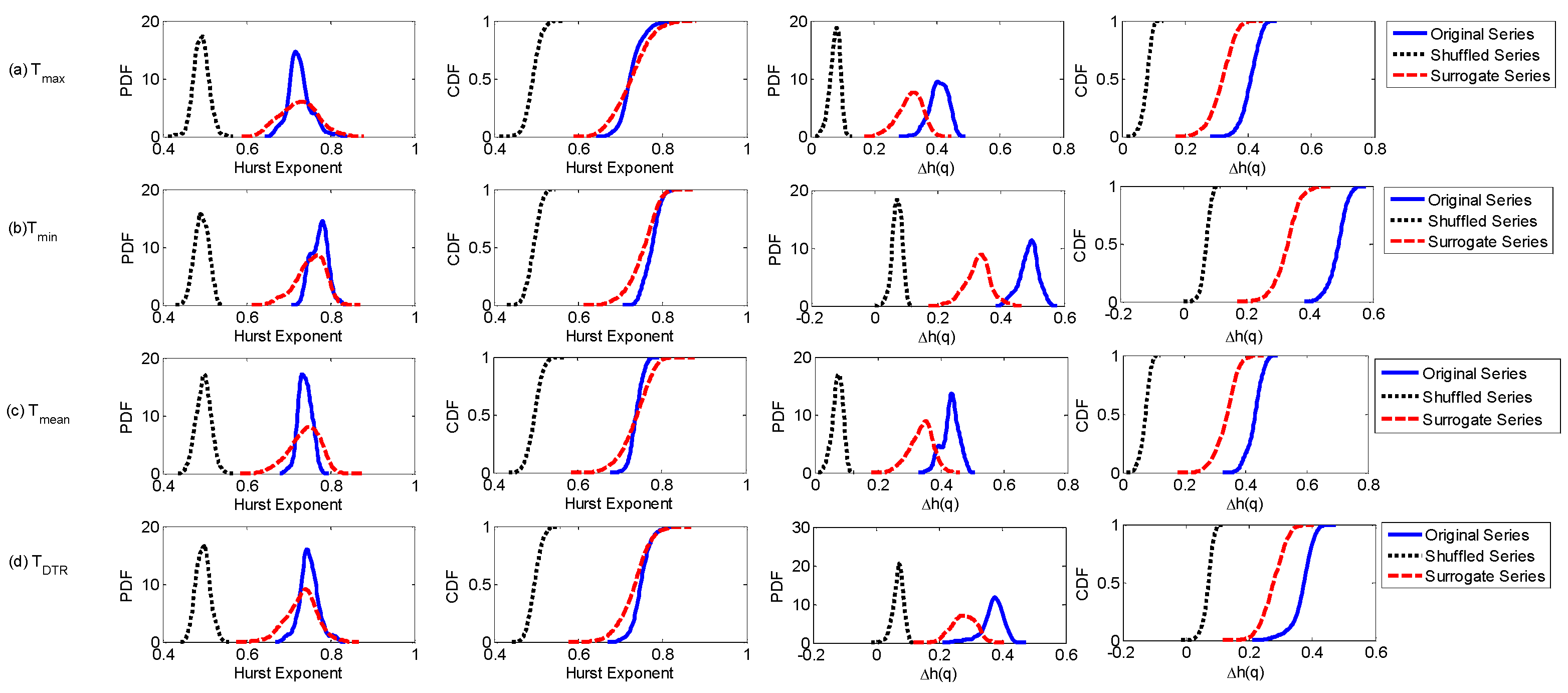
Identifying the underlying cause of multifractality is a crucial step in the multifractal analysis of hydro-meteorological series. The two major attributes of multifractal features are [46] the long range correlations and (ii) the broadness of the PDF. In this research work, the shuffling and surrogate were adopted to track the source of multifractality. The former operation eliminates the correlations in the time series, but by maintaining the same distributions. To estimate the role of the broadness of the PDF, a surrogacy operation was performed via phase randomization. The h(q) of the value for shuffled data was brought down to 0.5, which implies the role of correlation properties. If multifractal behavior is because of the broadness of the PDF, the h(q) of surrogate series will show q-independency [47]. If both causes are leading to multifractal behavior, the shuffled (SH) and surrogated (SU) series will show a lower multifractal property than the original (OR) series. The detailing on shuffling and phase randomization is available in the literature [48]. The GHE plots of the four temperature time series of all grid points are prepared for the OR, SH, and SU series. The Hurst exponent (H = h(2)) and ∆h(q) are estimated. The spatial variability of these parameters for original, shuffled, and surrogate series was quantified by developing the PDF and CDF of the estimates of different grid points. The plots are presented in Figure 3. From this figure, it is clear that the PDFs of the Hurst exponent of shuffled series are centered on 0.5. Also, from the CDFs, the variation in H is very small for shuffled series, and the variability of ∆h(q) is small (less than 0.1). Also, it is noticed that, for all the series, i.e., T_max, T_min, T_mean, and T_DTR, the CDFs of the ∆h(q) of the surrogate series are clearly to the left of those of the original series. Hence, it can be concluded that there is a clear dominance of the role of correlations in the multifractal behavior of the different temperature series over India, even though both the broadness of PDF and correlation properties are responsible.

4.2. Spatial Variability of Multifractal Characteristics of Temperature Datasets

To evaluate the spatial variability of the multifractal characteristics over the Indian mainland, firstly, the spatial distribution of the Hurst exponent and spectral width are presented in Figure 4, and similar plots of the Holder exponent and Asymmetry Index are presented in Figure 5.

Overall, in Figure 4, it is noticed that relatively lower persistence (H < 0.75) is dominant in the T_max, T_mean, and T_DTR series for approximately 82%, 65%, and 55% of the grid points. The Hurst exponent of the T_min series is higher than that of the other temperature series. The highest persistence (0.8–0.85) for T_min is noticed in the northern portion (like Utharakhand, Western Himalaya, and Lesser Himalaya–Sikkim) and southern tip of India. The Hurst exponent value of <0.75 is dominant in the regions of NC and NW, as well as the northern part of IP. In T_max − T_mean also, lower persistence is noticed in the NW region. On the contrary, in the T_DTR series, a higher H value is noted in a major portion of the NW region, meaning that the temperature-difference series is highly persistent in the desert-dominated NW region. In general, in the interior part of India (away from coastal areas), the fluctuations in temperature are more heterogeneous, while in the mountainous regions of Northern India, the behavior of the temperature is relatively homogeneous. Figure 4 demonstrates that, despite the presence of prevailing multifractal behavior, the predictability of such behavior is reasonably high in the NC, NW, and IP regions, where a high value of temperature tends to be followed by another high value. In the coastal zones, the predictability is more difficult, as such it is influenced by monsoon characteristics and ocean–land-surface interactions, and such processes have a great impact on the temperature. By examining Figure 4, it is further noticed that, consistently in all the four time series, high multifractal behavior is noticed in the northeastern coastal zone (comprising parts of EC, IP, NE, and NC) region. In the upper Himalaya region, the multifractal degree of all four temperature series is found to be the lowest.

By examining Figure 5, one can observe that the spectrum is near-symmetric (R is less and <0.2) for 89% of the grids for the T_DTR series and 68% for the T_max series. The behavior of the T_DTR series is quite different from the other three time series, and it resulted in a more symmetric spectrum (lower Asymmetry Index value) for most of the grid points. A strong asymmetry of the spectrum is noticed in the T_max − T_min − T_mean time series in the southern tip of India, comprising the coastal region and Peninsular India, whereas a near-symmetric spectrum resulted for the time series at the NW and NC. This indicates that the fluctuations in temperature extremes are more in the coastal belts and IP region, while extreme temperature episodes are practically repeated in a similar pattern in every year for Central India. All four temperature time series are found to be highly complex in the NE and the lesser Himalaya regions of India. High complexity is noticed in the T_max − T_min − T_mean of the WH, NW, and coastal regions, whereas a contrasting behavior in complexity is noted in the T_DTR series.

To understand the spatial variability in a more comprehensive way, the grid points in different regions and their multifractal properties were clustered. The EC, IP, WC, NE, NC, NW, and WH comprise 21, 84, 25, 25, 65, 54, and 5 grids, respectively. Then, the PDFs for the four multifractal parameters of the different time series were estimated, and the results are presented in Figure 6. In the WH region, only a few points are available. Consequently, the behavior of these PDFs will be less representative, and the results may not be reliable to make conclusions. Therefore, any further conclusions are based on the remaining six homogeneous regions (NC, NE, NW, WC, EC, and IP).

In Figure 6, it can be observed that the lowest range of Hurst exponents belongs to the NC region for all the series, and the density is highest for the T_min and T_DTR series. Furthermore, the perusal of the plot reveals that the spread of the Hurst exponent is the highest for the WC area, where the predictability of temperature is quite difficult. However, to a lesser degree, this is also noticeable in the eastern coast for some of the series. For example, the spread of PDFs for H in the EC region is more significant, so the predictability of the T_min series is quite difficult in this area. Figure 6 illustrates that the PDF of the spectral width in the NC region is quite similar to that of the NW region for all series except T_max, whereas it exhibits a remarkable resemblance to the IP area for the T_max series. The range of all the multifractal parameters is the highest in the WC region. This behavior could be linked to the oceanic proximity and the changes in the temperature due to climatic characteristics like monsoon. To sum up, the variability in multifractal properties is the lowest in the NC region, followed by the NW region, while it is highest in the WC area. To obtain more insight into the properties for the different regions, the statistical characteristics, like the mean, standard deviation (SD), and coefficient of variation (CV), of the multifractal parameters were computed and are presented in

Table 2. Statistical summary (mean, standard deviation (SD), and coefficient of variation (CV)) of multifractal properties for temperature series of different temperature-homogeneous regions of India. In the regional-scale analysis, the highest variability is marked in italics, and the lowest variability is marked in bold.

Temperature Series	Region	Hurst Exponent			Spectral Width			Asymmetry Index			Holder Exponent
		Mean	SD	CV (%)	Mean	SD	CV (%)	Mean	SD	CV (%)	Mean	SD	CV (%)
Tmin	EC	0.756	0.022	2.861	0.652	0.054	8.326	0.158	0.040	25.673	0.819	0.028	3.371
	IP	0.747	0.016	2.120	0.692	0.035	5.113	0.202	0.055	27.061	0.815	0.018	2.178
	NC	0.793	0.009	1.176	0.655	0.027	4.082	0.273	0.034	12.479	0.844	0.013	1.598
	NE	0.804	0.025	3.072	0.663	0.032	4.809	0.231	0.031	13.248	0.875	0.020	2.332
	NW	0.782	0.015	1.857	0.627	0.028	4.514	0.259	0.043	16.436	0.851	0.007	0.798
	WC	0.758	0.016	2.135	0.656	0.039	5.905	0.183	0.038	20.575	0.820	0.019	2.339
Tmax	EC	0.732	0.026	3.579	0.586	0.037	6.338	0.125	0.030	23.635	0.777	0.022	2.863
	IP	0.721	0.025	3.490	0.591	0.046	7.739	0.116	0.032	27.515	0.773	0.021	2.712
	NC	0.713	0.024	3.383	0.591	0.044	7.507	0.224	0.079	35.222	0.762	0.021	2.700
	NE	0.719	0.023	3.148	0.591	0.057	9.669	0.210	0.066	31.697	0.771	0.017	2.164
	NW	0.725	0.026	3.580	0.576	0.039	6.849	0.228	0.075	32.835	0.769	0.024	3.178
	WC	0.711	0.050	7.073	0.564	0.030	5.345	0.129	0.062	48.181	0.758	0.052	6.871
Tmean	EC	0.743	0.013	1.713	0.578	0.047	8.101	0.180	0.038	21.337	0.788	0.012	1.582
	IP	0.726	0.013	1.764	0.594	0.040	6.660	0.178	0.030	16.749	0.776	0.012	1.535
	NC	0.743	0.013	1.765	0.622	0.025	3.949	0.252	0.035	13.763	0.795	0.014	1.725
	NE	0.755	0.016	2.182	0.626	0.030	4.858	0.231	0.022	9.551	0.813	0.016	1.940
	NW	0.758	0.013	1.753	0.611	0.019	3.092	0.235	0.039	16.376	0.810	0.012	1.504
	WC	0.713	0.021	2.909	0.570	0.054	9.496	0.164	0.063	38.494	0.763	0.022	2.900
TDTR	EC	0.746	0.024	3.163	0.492	0.037	7.428	0.131	0.031	23.676	0.784	0.026	3.360
	IP	0.742	0.019	2.534	0.547	0.045	8.266	0.105	0.049	46.355	0.788	0.019	2.355
	NC	0.745	0.010	1.356	0.570	0.028	4.835	0.122	0.040	32.837	0.794	0.009	1.158
	NE	0.787	0.028	3.599	0.578	0.038	6.512	0.125	0.034	27.527	0.835	0.024	2.851
	NW	0.732	0.027	3.629	0.550	0.020	3.693	0.102	0.035	34.241	0.779	0.026	3.346
	WC	0.769	0.022	2.924	0.512	0.057	11.082	0.146	0.036	24.807	0.809	0.019	2.309

. For better clarity, a visual examination is also made by plotting the CDFs (see Figure 7) of the estimates for the four multifractal parameters based on the grids falling within the different homogeneous regions.

For the T_min series (see Table 2), the variability of all the multifractal properties is the lowest in NC region. For the T_DTR series, the variability of all multifractal properties, except asymmetry, is also the lowest in NC region. Considering the T_mean series, all the multifractal properties show the highest variability in the WC region, contrary to the other series. It is to be recollected that, for all the grid points, i.e., All India (AI), the highest variability in persistence (3.91), and the multifractal degree (9.19) is noted for DTR series, while the highest variability in complexity and asymmetry is noticed for the T_max series (Table 1). Also, the variability in all four properties is the lowest in the T_mean series. From the CDF plots, it is evident that the persistence is highest in NE for all temperature series except T_max, which shows a fairly homogeneous pattern of this temperature in the NE area. Even though a relatively larger H value is noted in the NW region for the DTR series, the persistence is lowest in this area. This highlights the rich dynamics between T_max and T_min in the desert located in the NW region. In the spectral width, there is no consistent pattern, but for T_min and T_DTR, the multifractal degree is relatively higher in the NE and NC regions. High complexity is also noticed in the time series of the NE region for all four temperature series. Lower complexity and asymmetry are observed in the time series for the WC region in all the time series except DTR. Overall, there is a no unique pattern, and there exists spatial diversity in the multifractal characteristics of the four different temperature series.

4.3. Temporal Change in Multifractal Properties

The temporal changes in the multifractal properties are crucial because they give information about the changing characteristics of the time series. These drastic changes in properties can be signatures of climate change [49], and in such a context, it will be useful to follow appropriate modeling practices to improve the accuracy of predictions. A possible reason for these changes in multifractal properties could be the urbanization, as it might be leading to a more irregular profile and, thus, the smoothening and subsequent reduction of multifractality [50]. Urban areas with a more irregular surface profile and heat emission can lead to complex temperature profiles possessing a high degree of multifractality. It is further assumed that the change could also be related to climate factors as well. Researchers have identified a well-debated climate change in the Pacific during the period 1976–1977 and the subsequent change in global temperature [51,52]. To investigate the role of climatic shift, all four temperature time series were split into the pre- and post-1977 period, and an MFDFA was performed. The CDFs of prominent multifractal characteristics were computed and are presented in Figure 8.

Figure 8 shows that there is an evident reduction in the multifractality, persistence, and complexity for the series of post-1977 global climate shift (GCS). It can be noticed that there is no definite pattern in the shape of the multifractal spectra for the different series of the pre- and post-1976–1977 period, except for T_DTR and T_mi: the left or right truncation (which indicates the frequency of existence of extremes) was displayed randomly in different grid points. Furthermore, the reduction of R in the T_DTR series for the post-1976–1977 series is rather marginal. This highlights the more homogeneous nature of the diurnal temperature series in the post-1976–1977 GCS period. The α₀ values of all the four types of daily temperature series displayed a systematic reduction for the post-1976–1977 GCS period. This is contrary to the observations made by Krzyszczak et al. [49] on the property of the time series of different meteorological parameters in Europe, which was mainly controlled by the local changes in climate dynamics. Thus, it can be inferred that the non-linearity and multifractality of Indian temperature is controlled to a large extend by the global climate dynamics and the Indian monsoon system. Many studies have highlighted an increasing trend in the T_min series in India during the second half of the last century, and some researchers have reported that the variability in the T_min is quite different from that of the T_max based on detection and attribution studies [53]. Overall, it is evident that there is a notable destruction in persistence properties and multifractal behavior for the series from the period after 1977, and these changes in multifractal properties of different temperature series over India may be attributed to climate change and urbanization.

4.4. Multifractal Analysis in 10-Year Rolling Window

In this section, we conduct an analysis using a 10-year rolling window to capture the evolution of multifractal properties across the time domain. The values of the exponents α_max, α_min, and α₀, which are the projection of the multifractal spectrum onto the x-axis, are presented in Figure 9, Figure 10, Figure 11 and Figure 12. One could clearly observe that they are dynamic in the time domain. Instances where the spectrum becomes narrower are highlighted with dotted circles. A narrowed spectrum is associated with weak multifractal correlations in the examined time series and could signify a potential shift in regime [54, 55]. This was observed for T_max, T_min, and T_mean in 10-year rolling windows from 1985 until 1995 and for T_max even in 2001 and 2010. Especially in the case of the T_mean for the NC and NE regions during the period 1985–1995, the spectra are close to a point, indicating the mono-fractal nature of the series. For the T_min in the NC and NE regions, one can notice that the left side of the spectrum is reduced to a point during the same period. For the T_max, we could also observe a very narrow spectrum from 1965 to 1974. This may indicate some potential regime changes, especially for T_max. For T_DTR, one can observe that the spectra were wider during the period 1985–1995. This distinct behavior, unlike other temperature measures, may result from the interplay between maximal and minimal temperature changes. The spectrum takes on a different shape, particularly in the WH region, where only a few points are located, potentially causing disturbances in the results.

Based on the MFDFA analysis, we can also distinguish the changes in the Hurst exponent over time. Its temporal evolution for all the seven regions is presented in Figure 13 (T_max, T_min) and Figure 14 (T_DTR, T_mean). By comparing these two Figures, it is clearly visible that the H values are higher for T_DTR and T_mean (Figure 14) than T_max and T_min (Figure 13). The lowest H values can be observed for T_max, and they are also the most volatile during the considered time period. The declining trend and the Hurst exponent approaching a value of 0.6 are particularly noticeable for T_max in all regions within rolling windows ending from 1971 to 1977. There is also a less pronounced but still present intensity in certain regions from 1990 to 2000 and from 2010 to 2016. This provides valuable insights into regions potentially more susceptible to climatic change, exhibiting a faster pace of transformation. It is well understood that both the T_max and T_min rise because of global changes in climate, despite the changes in the rates of increase with respect to climate zones [44]. In the drylands, semi-arid and warm grasslands of India, the rate of rise in the T_min is more than that of the T_max. Sub-tropical forests, equatorial grasslands down south, and the WC show an opposing behavior. In general, the coastal and peninsular regions show the highest change in T_max and T_DTR series, while the northwest region shows the highest change in T_min.

In this research, we applied the MFDFA analysis to study the complex fluctuations and scaling of daily temperature data in various regions of India from 1951 to 2016. It is noteworthy that our study is the most comprehensive, encompassing all four types of temperature series (T_max, T_min, T_mean, and T_DTR) and spanning the entire spatial domain of the Indian mainland. The multifractal spectra for the whole considered period have right-sided asymmetry. The time series are well persistent also, with H values well above 0.6 in all cases. The multifractal characteristics of temperature can be attributed to the physical mechanisms that lead to it. In addition to global parameters such as the sunspot number, earth rotation, solar and terrestrial radiations, local factors such as latitude, atmospheric and oceanic oscillations, and topographic features may contribute to the emergence of multifractality in the series. The proximity to oceans significantly influences the precipitation in India, as the country is surrounded by the Arabian Sea, Indian Ocean, and Bay of Bengal in its western, southern, and eastern regions. However, it will be difficult to find a universal pattern in the changes in the scaling exponent and multifractal properties with distance from the coast and the latitude and altitude. Moreover, attributing multifractality to a single indicator is challenging due to the complexity of the Indian monsoon system and the influence of local processes and factors, such as terrain type, moisture, and vegetation, on regional precipitation variations. It has been well established that global and regional temperatures are influenced by the El Niño Southern Oscillation (ENSO). In addition, the large-scale atmospheric circulations of diverse periodicities play a main role on the southwest monsoon rainfall of India in the summer season [56]. A more insightful depiction of multifractal dynamics can be obtained through the study by conducting the analysis from a rolling-window perspective. Our results clearly show that the multifractal characteristics and H values are dynamic over the time domain. Observations based on multifractal spectrum width changes may indicate some regime shifts, especially for T_max and T_mean during the 1980s and 2000s. These results are supported by the behavior of Hurst exponent, whose values have declined during this period. Drawing conclusions from the presented results, one could infer potential climate changes and global regime shifts in the mentioned decades.

While the multifractal characteristics of hydrological and meteorological time series are widely discussed in the literature, the practical application and dissemination of these parameters for simulation or prediction purposes are still relatively limited. Some studies have demonstrated the link between persistence and predictability and the autocorrelation values of the time series [57,58]. Understanding the multifractal properties can be effectively used in the multifractal modeling, simulation, and synthetic generation of hydro-meteorological fields and de-noising of hydro-meteorological signals [59,60]. Multifractal properties can be considered promising tools for homogeneity detection and frequency analysis [35,61]. Analyzing the spatial and temporal variability of multifractal properties has a lot of practical significance, as it may help in detecting the mechanisms and the inter arrival times of hydrologic extremes and heat waves. Moreover, the escalating global temperature is a significant concern, and its pattern is becoming more intricate, introducing non-stationary features. This emphasizes the need to construct temperature–duration–frequency (TDF) curves using robust methods to address heatwave and drought disasters [62]. Any significant change in persistence could affect the accuracy of predictions, similar to relying on a stationarity assumption in a non-stationary setting resulting from climatic changes. This innovative approach will empower hydrologists to delve deeper into multifractal and non-stationary modeling methods, fostering additional research in the field.

5. Conclusions

In this study, we employed the Multifractal Detrended Fluctuation Analysis (MFDFA) method to investigate the scaling behavior of daily temperature series across India, along with the analysis on their spatial and temporal variability. High-resolution datasets for maximum temperature (T_max), minimum temperature (T_min), mean temperature (T_mean), and diurnal temperature range (T_max–T_min) spanning the period 1951–2016 at daily temporal scales were utilized. The key findings are summarized as follows:

•

All four types of temperature series (T_max, T_min, T_mean, and T_DTR) in India exhibited strong long-term persistence;

•

Among the four temperature series, T_min displayed the highest persistence and degree of multifractality;

•

The variability of multifractal characteristics was lowest in North–Central India and highest in the West Coast region;

•

A noticeable decrease in persistence and multifractal properties was observed in India’s temperature series following the Pacific climatic shift of 1976–1977;

•

The multifractal properties observed in the temperature series across India can be attributed more to the dominant influence of correlation properties rather than the shape of the probability density function;

•

The temporal evolution analysis of multifractality successfully captured the climatic shifts of 1976–1977 and 1998–1999;

•

The climatic shift in the 1980s predominantly alleviated the persistence of the T_max series, while the shift in 1998 had a dominant effect on influencing the persistence of the T_mean series in the majority of temperature-homogeneous regions in India.

All of these results provide valuable insights into the improved understanding of the impact of climate change across the Indian mainland.

References

- Shang, P.; Kame, S. Fractal nature of time series in the sediment transport phenomenon. Chaos Solitons Fractals 2005, 26, 997–1007. [Google Scholar] [CrossRef]
- Kantelhardt, J.W.; Bunde, E.K.; Rybski, D.; Barun, P.; Bunde, A.; Havlin, S. Long-term persistence and multifractality of precipitation and river runoff records. J. Geophys. Res. Atmos. 2006, 28, 1–13. [Google Scholar]
- Hurst, H.E. Long-term storage capacity of reservoirs. Trans. ASCE 1951, 116, 770–808. [Google Scholar] [CrossRef]
- Mandelbrot, B. The Fractal Geometry of Nature; WH Freeman Publishers: New York, NY, USA, 1982. [Google Scholar]
- Tessier, Y.; Lovejoy, S.; Hubert, P.; Schertzer, D.; Pecknold, S. Multifractal analysis and modeling of rainfall and river flows and scaling, causal transfer functions. J. Geophys. Res. Atmos. 1996, 101, 26427–26440. [Google Scholar] [CrossRef]
- Pandey, G.; Lovejoy, S.; Schertzer, D. Multifractal analysis of daily river flows including extremes for basins five to two million square kilometres, one day to 75 years. J. Hydrol. 1998, 208, 62–81. [Google Scholar] [CrossRef]
- Dahlstedt, K.; Jensen, H. Fluctuation spectrum and size scaling of river flow and level. Phys. A Stat. Mech. Its Appl. 2005, 348, 596–610. [Google Scholar] [CrossRef]
- Kantelhardt, J.W.; Rybski, D.; Zschiegner, S.A.; Braun, P.; Koscielny-Bunde, E.; Livina, V.; Havlin, S.; Bunde, A. Multifractality of river runoff and precipitation: Comparison of fluctuation analysis and wavelet methods. Phys. A Stat. Mech. Its Appl. 2003, 330, 240–245. [Google Scholar] [CrossRef]
- Peng, C.K.; Buldyrev, S.V.; Simons, M.; Stanley, H.E.; Goldberger, A.L. Mosaic organization of DNA nucleotides. Phys. Rev. E 1994, 49, 1685–1689. [Google Scholar] [CrossRef]
- Kantelhardt, J.W.; Zschiegner, S.A.; Koscielny-Bunde, E.; Halvin, H.; Bunde, A.; Stanley, H.E. Multifractal detrended fluctuation analysis of non-stationary time series. Phys. A Stat. Mech. Its Appl. 2002, 316, 87–114. [Google Scholar] [CrossRef]
- Eichner, J.F.; Koscielny-Bunde, E.; Bunde, A.; Schellnhuber, H.J. Power-law persistence and trends in the atmosphere: A detailed study of long temperature records. Phys. Rev. E 2003, 68 Pt 2, 046133. [Google Scholar] [CrossRef]
- Mali, P. Multifractal characterization of global temperature anomalies. Theor. Appl. Climatol. 2015, 121, 641–648. [Google Scholar] [CrossRef]
- Lin, G.; Chen, X.; Fu, Z. Temporal–spatial diversities of long-range correlation for relative humidity over China. Phys. A Stat. Mech. Its Appl. 2007, 383, 585–594. [Google Scholar] [CrossRef]
- Liu, Z.; Xu, J.; Chen, Z.; Nie, Q.; Wei, C. Multifractal and long memory of humidity process in the Tarim River Basin. Stoch. Environ. Res. Risk Assess. 2014, 28, 1383–1400. [Google Scholar] [CrossRef]
- Yu, Z.G.; Leung, Y.; Chen, Y.D.; Zhang, Q.; Anh, V.; Zhou, Y. Multifractal analyses of daily rainfall time series in Pearl River basin of China. Phys. A Stat. Mech. Its Appl. 2014, 405, 193–202. [Google Scholar] [CrossRef]
- Baranowski, P.; Krzyszczak, J.; Slawinski, C.; Hoffmann, H.; Kozyra, J.; Nieróbca, A.; Siwek, K.; Gluza, A. Multifractal analysis of meteorological time series to assess climate impacts. Clim. Res. 2015, 65, 39–52. [Google Scholar] [CrossRef]
- Gómez-Gómez, J.; Carmona-Cabezas, R.; Sánchez-López, E.; Gutiérrez de Ravé, E.; Jiménez-Hornero, F.J. Multifractal fluctuations of the precipitation in Spain (1960–2019). Chaos Solitons Fractals 2022, 157, 111909. [Google Scholar] [CrossRef]
- Koscielny-Bunde, E.; Kantelhardt, J.W.; Braun, P.; Bunde, A.; Havlin, S. Long-term persistence and multifractality of river runoff records: Detrended fluctuation studies. J. Hydrol. 2003, 322, 120–137. [Google Scholar] [CrossRef]
- Zhang, Q.; Xu, C.Y.; Chen, D.Y.Q.; Gemmer, M.; Yu, Z.G. Multifractal detrended fluctuation analysis of streamflow series of the Yangtze River basin, China. Hydrol. Process. 2008, 22, 4997–5003. [Google Scholar] [CrossRef]
- Zhang, Q.; Chong, Y.X.; Yu, Z.G.; Liu, C.L.; Chen, D.Y.Q. Multifractal analysis of streamflow records of the East River basin (Pearl River), China. Phys. A Stat. Mech. Its Appl. 2009, 388, 927–934. [Google Scholar] [CrossRef]
- Li, E.; Mu, X.; Zhao, G.; Gao, P. Multifractal detrended fluctuation analysis of streamflow in Yellow river basin, China. Water 2015, 7, 1670–1686. [Google Scholar] [CrossRef]
- Sankaran, A.; Krzyszczak, J.; Baranowski, P.; Devarajan Sindhu, A.; Kumar, N.P.; Lija Jayaprakash, N.; Thankamani, V.; Ali, M. Multifractal cross correlation analysis of agro-meteorological datasets (including reference evapotranspiration) of California, United States. Atmosphere 2020, 11, 1116. [Google Scholar] [CrossRef]
- Adarsh, S.; Nityanjaly, L.J.; Sarang, R.; Pham, Q.B.; Ali, M.; Nandhineekrishna, P. Multifractal Characterization and Cross correlations of Reference Evapotranspiration Time Series of India. Eur. Phys. J. Spec. Top. 2021, 230, 3845–3859. [Google Scholar] [CrossRef]
- Gómez-Gómez, J.; Ariza-Villaverde, A.B.; Gutiérrez de Ravé, E.; Jiménez-Hornero, F.J. Relationships between Reference Evapotranspiration and Meteorological Variables in the Middle Zone of the Guadalquivir River Valley Explained by Multifractal Detrended Cross-Correlation Analysis. Fractal Fract. 2023, 7, 54. [Google Scholar] [CrossRef]
- Sankaran, A.; Plocoste, T.; Nourani, V.; Vahab, S.; Salim, A. Assessment of Multifractal Fingerprints of Reference Evapotranspiration Based on Multivariate Empirical Mode Decomposition. Atmosphere 2023, 14, 1219. [Google Scholar] [CrossRef]
- Zhang, Q.; Lu, W.; Chen, S.; Liang, X. Using multifractal and wavelet analyses to determine drought characteristics: A case study of Jilin province, China. Theor. Appl. Climatol. 2016, 125, 829–840. [Google Scholar] [CrossRef]
- Adarsh, S.; Kumar, D.N.; Deepthi, B.; Gayathri, G.; Aswathy, S.S.; Bhagyasree, S. Multifractal characterization of meteorological drought in India using detrended fluctuation analysis. Int. J. Climatol. 2019, 39, 4234–4255. [Google Scholar] [CrossRef]
- Zhan, C.; Liang, C.; Zhao, L.; Jiang, S.; Niu, K.; Zhang, Y. Multifractal characteristics of multiscale drought in the Yellow River Basin, China. Phys. A Stat. Mech. Its Appl. 2023, 609, 128305. [Google Scholar] [CrossRef]
- Lin, G.; Fu, Z. A universal model to characterize different multi-fractal behaviors of daily temperature records over China. Phys. A Stat. Mech. Its Appl. 2008, 387, 573–579. [Google Scholar] [CrossRef]
- Yuan, N.; Fu, Z.; Mao, J. Different scaling behaviors in daily temperature records over China. Phys. A Stat. Mech. Its Appl. 2010, 389, 4087–4095. [Google Scholar] [CrossRef]
- Orun, M.; Kocak, K. Applicatıon of detrended fluctuation analysis to temperature data from Turkey. Int. J. Climatol. 2009, 29, 2130–2136. [Google Scholar] [CrossRef]
- Kalamaras, N.; Philippopoulos, K.; Deligiorgi, D.; Tzanis, C.G.; Karvounis, G. Multifractal scaling properties of daily air temperature time series. Chaos Solitons Fractals 2017, 98, 38–43. [Google Scholar] [CrossRef]
- Burgueño, A.; Lana, X.; Serra, C.; Martínez, M.D. Daily extreme temperature multifractals in Catalonia (NE Spain). Phys. Lett. A 2014, 378, 874–885. [Google Scholar] [CrossRef]
- Herrera-Grimaldi, P.; García-Marín, A.P.; Estévez, J. Multifractal analysis of diurnal temperature range over Southern Spain using validated datasets. Chaos 2019, 29, 063105. [Google Scholar] [CrossRef] [PubMed]
- Garcia-Marin, A.P.; Morbidelli, R.; Saltalippi, C.; Cifrodelli, M.; Esteveza, J.; Flammini, A. On the choice of the optimal frequency analysis of annual extreme rainfall by multifractal approach. J. Hydrol. 2019, 575, 1267–1279. [Google Scholar] [CrossRef]
- da Silva, H.S.; Silva, J.R.S.; Stosic, T. Multifractal analysis of air temperature in Brazil. Phys. A Stat. Mech. Its Appl. 2020, 549, 124333. [Google Scholar] [CrossRef]
- Purnadurga, G.; Kumar, T.V.L.; Rao, K.K.; Rajasekhar, M. Investigation of temperature changes over India in association with meteorological parameters in a warming climate. Int. J. Climatol. 2018, 38, 867–877. [Google Scholar] [CrossRef]
- Yasunaka, S.; Hanawa, K. Regime Shift in the Global Sea-Surface Temperatures: Its Relation to ElNinO–Southern Oscillation Events and Dominant Variation Mode. Int. J. Climatol. 2005, 25, 913–930. [Google Scholar] [CrossRef]
- Sarkar, S.; Maity, R. Global climate shift in 1970s causes a significant worldwide increase in rainfall extremes. Sci. Rep. 2021, 11, 11574. [Google Scholar] [CrossRef] [PubMed]
- Srivastava, A.K.; Rajeevan, M.; Kshirsagar, S.R. Development of a high resolution daily gridded temperature data set (1969–2005) for the Indian region. Atmos. Sci. Lett. 2009, 10, 249–254. [Google Scholar] [CrossRef]
- Shepard, D. A two-dimensional interpolation function for irregularly spaced data. In Proceedings of the 1968 23rd ACM National Conference, New York, NY, USA, 1 January 1968; pp. 517–524. [Google Scholar]
- Willmott, C.; Matsuura, K.T.A. Temperature and Precipitation: Monthly and Annual Time Series (1950–1999), at 2001. Available online: http://www.esrl.noaa.gov/psd/data/gridded/data.UDel_AirT_Precip.html (accessed on 11 April 2022).
- Rajeevan, M.; Bhate, J.; Kale, J.; Lal, B. Development of a High-Resolution Daily Gridded Rainfall Data for the Indian Region; Government of India, India Meteorological Department: Pune, India, 2005; Research Report 22/2005.
- Vinnarasi, R.; Dhanya, C.T.; Chakravorthy, A.; Aghakouchak, A. Unravelling diurnal asymmetry of surface temperature in different climate zones. Sci. Rep. 2017, 7, 7350. [Google Scholar] [CrossRef]
- Drożdż, S.; Oświęcimka, P. Detecting and interpreting distortions in hierarchical organization of complex time series. Phys. Rev. E 2015, 91, 030902(R). [Google Scholar] [CrossRef]
- Movahed, M.S.; Jafari, G.R.; Ghasemi, F.; Rahvar, S.; Tabar, M.R.R. Multifractal detrended fluctuation analysis of sunspot time series. J. Stat. Mech. 2006, 2, P02003. [Google Scholar] [CrossRef]
- Matia, K.; Ashkenazy, Y.; Stanley, H.E. Multifractal properties of price fluctuations of stocks and commodities. Europhys. Lett. 2003, 61, 422–428. [Google Scholar] [CrossRef]
- Hou, W.; Feng, G.; Yan, P.; Li, S. Multifractal analysis of the drought area in seven large regions of China from 1961 to 2012. Meteorol. Atmos. Phy. 2017, 130, 459–471. [Google Scholar] [CrossRef]
- Krzyszczak, J.; Baranowski, P.; Zubik, M.; Kazandjiev, V.; Georgieva, V.; Sławiński, C.; Siwek, K.; Kozyra, J.; Nieróbca, A. Multifractal characterization and comparison of meteorological time series from two climatic zones. Theor. Appl. Climatol. 2019, 137, 1811–1824. [Google Scholar] [CrossRef]
- Karatasou, S.; Santamouris, M. Multifractal analysis of high-frequency temperature time series in the urban environment. Climate 2018, 6, 50. [Google Scholar] [CrossRef]
- Miller, A.J.; Cayan, D.R.; Barnett, T.P.; Oberhuber, J.M. The 1976–77 Climate Shift of the Pacific Ocean. Oceanography 1994, 7, 21–26. [Google Scholar] [CrossRef]
- Sahana, A.S.; Ghosh, S.; Ganguly, A.; Murtugudde, R. Shift in Indian summer monsoon onset during 1976/1977. Environ. Res. Lett. 2015, 10, 054006. [Google Scholar] [CrossRef]
- Sonali, P.; Kumar, D.N. Detection and Attribution of Seasonal Temperature Changes in India with Climate Models in the CMIP5 Archive. J. Water Clim. Chang. 2016, 7, 83–102. [Google Scholar] [CrossRef]
- Drożdż, S.; Kowalski, R.; Oświȩcimka, P.; Rak, R.; Gȩbarowski, R. Dynamical Variety of Shapes in Financial Multifractality. Complexity 2018, 2018, 7015721. [Google Scholar] [CrossRef]
- Grech, G.; Mazur, Z. Can one make any crash prediction in finance using the local Hurst exponent idea? Phys. A Stat. Mech. Its Appl. 2004, 336, 133–145. [Google Scholar] [CrossRef]
- Gadgil, S.; Vinayachandran, P.N.; Francis, P.A.; Gadgil, S. Extremes of the Indian summer monsoon rainfall, ENSO and equatorial Indian Ocean oscillation. Geophys. Res. Lett. 2004, 31, L12213. [Google Scholar] [CrossRef]
- Bassingthwaighte, J.B.; Beyer, R.P. Fractal correlation in heterogeneous systems. Phys. D 1991, 53, 71–84. [Google Scholar] [CrossRef]
- Chandrasekharan, S.; Saminathan, B.; Suthanthiravel, S.; Sundaram, S.K.; Hakkim, F.F.A. An investigation on the relationship between the Hurst exponent and the predictability of a rainfall time series. Meteorol. Appl. 2019, 26, 511–519. [Google Scholar] [CrossRef]
- Deidda, R.; Benzi, R.; Siccardi, F. Multifractal modeling of anomalous scaling laws in rainfall. Water Resour. Res. 1999, 35, 1853–1867. [Google Scholar] [CrossRef]
- Cadenas, E.; Campos-Amezcua, R.; Rivera, W.; Espinosa-Medina, M.A.; Méndez-Gordillo, A.R.; Rangel, E.; Tena, J. Wind speed variability study based on the Hurst coefficient and fractal dimensional analysis. Energy Sci. Eng. 2019, 7, 361–378. [Google Scholar] [CrossRef]
- García-Marín, A.P.; Estévez, J.; Medina-Cobo, M.T.; Ayuso-Muñoz, J.L. Delimiting homogeneous regions using the multifractal properties of validated rainfall data series. J. Hydrol. 2015, 529, 106–119. [Google Scholar] [CrossRef]
- Mohan, M.G.; Adarsh, S. Development of non-stationary temperature duration frequency curves for Indian mainland. Theor. Appl. Climatol. 2023, 154, 999–1011. [Google Scholar] [CrossRef]
Figure 1.
Map showing seven temperature-homogeneous regions in India.
Figure 2.
PDFs (left panels) and CDFs (right panels) of multifractal characteristics (Hurst exponent, spectral width, Asymmetry Index, and Holder exponent) for the four temperature time series: Tmax, Tmin, Tmean, and TDTR.
Figure 3.
PDFs and CDFs of Hurst exponent and spectral width for original, surrogate, and shuffled series of four temperature records.
Figure 4.
The spatial distribution of Hurst exponent (upper panel) and spectral width (lower panel) for the four temperature series.
Figure 5.
Spatial distribution of Asymmetry Index (upper panel) and Holder exponent (lower panel) for the four temperature series.
Figure 6.
PDFs of multifractal parameters for the different temperature series according to the homogeneous regions in India.
Figure 7.
CDFs of multifractal parameters for the different temperature series in different homogeneous regions in India.
Figure 8.
CDFs of multifractal characteristics for the different temperature time series of pre- and post-1977 global climatic shift for (a) Hurst exponent, (b) spectral width, (c) Asymmetry Index, and (d) Holder exponent.
Figure 9.
Temporal variability of exponents of multifractal spectra for Tmax series averaged over grid points belonging to seven homogeneous regions. The circled regions show the years of evident climate change while the vertical dashed lines exhibited the identified prominent global climate shift.
Figure 10.
Temporal variability of exponents of multifractal spectra for Tmin series averaged over grid points belonging to seven homogeneous regions. The circled regions show the years of evident climate change.
Figure 11.
Temporal variability of exponents of multifractal spectra for Tmean averaged over grid points belonging to seven homogeneous regions. The circled regions show the years of evident climate change.
Figure 12.
Temporal variability of exponents of multifractal spectra for TDTR series averaged over grid points belonging to seven homogeneous regions. The circled regions show the years of evident climate change while the vertical dashed lines exhibited the identified prominent global climate shift.
Figure 13.
Temporal variability of Hurst exponents for Tmax and Tmin averaged over grid points belonging to the regions. The circled regions show the years of evident climate change.
Figure 14.
Temporal variability of Hurst exponents for TDTR and Tmean averaged over grid points belonging to the regions. The circled regions show the years of evident climate change.