Optimal Missing Value Estimation Algorithm for Groundwater Levels ^†

Abstract

In this study an algorithm for missing data imputation is presented. The algorithm uses measurements from neighboring sensors to estimate the missing values. Data-driven approach is used and methodology chooses the optimal available combination of modeling algorithm and available measurements to produce an estimate from the model with lowest error. The methodology was tested on Ljubljana polje aquifer data and has produced close to perfect results.

1. Introduction

Groundwater is an important indicator of changes in the climate. To assess the changes in comparison to groundwater withdrawal and different land-use long term availability of the data is needed. Usually different sensors for measuring groundwater levels are active in different time periods and might be subjected to very different properties of collected data (frequency, precision, etc.). In this paper a missing value estimation algorithm based on available data from active near-by sources is presented and tested it on data available from Ljubljana aquifer. Groundwater level measurements for Ljubljana aquifer are quite sparse. First measurements have been conducted in 1949 by one sensor and no sensor has measured groundwater levels continuously up until the present day. There are time intervals with more active sensors (1967–1971, 2002–2017), however—in between only a few sensors have been recording measurements. Additionally—each sensor has random missing values during the intervals, when measurements have been taken and also frequencies of data measurements change significantly between different time periods.

There are a plethora of reasons for missing data: hardware or software malfunction, human error (in the early measurements of groundwater levels), intentional removal (when data is corrupted). We choose the process of data imputation to deal with missing values, which means that we want to approximate the missing data points. There are many different ways to impute missing values. A missing value can be substituted with a mean, with a substitute from another individual, from a hot deck (randomly chosen value from an individual who has similar properties), cold-deck (like in hot-deck, but the individual is chosen systematically), with regression (based on other variables), stochastic regression (adding a random residual value to regression), with interpolation and extrapolation (estimate from the other observations from the same individual).

Missing data of sparsely sampled time-series can be imputed with the usage of regression trees [1]. Such models rely on nearby sensors’ measurements and use linear interpolation at a pre-processing step to improve model accuracies. The methodology, described in this paper, also uses linear regression interpolation within a sparse datasets, but also propose usage of b-splines. In addition to regression trees we also test other methods like linear regression, random forests and support vector machines. We propose the usage of the optimal algorithm and optimal feature set.

Simple (interpolation with last value and mean) and sophisticated methods, such as linear regression and PCA are also applicable in missing data imputation scenario [2]. Tensor-based methods also produce very good results in estimating missing values [3]. In some cases, where data of one or several days were completely missing, missing values were successfully imputed with this method.

Short-term Kalman filter models are suitable for imputation of missing or corrupt time-series data in a streaming scenario [4]. The method is suitable for detection and substitution of single outliers with linear methods, whereas our approach can substitute larger chunks of missing data with more complex methods. The approach, presented in this paper, could be extended into outlier detection algorithm.

In groundwater missing data imputation authors of [5] suggested groundwater nitrate monitoring network optimization with reduction of measuring nodes. They estimate errors at missing nodes with linear methods to substitute measurements. In our work we take a similar approach, but do not care about network reduction.

Hot-deck imputation method can be used on a global scale [6]. Missing values are replaced with a value from the donor cases, which match the recipient node in a set of specified variables from the same dataset. Value is chosen randomly or from the deck with the closes similarity. In our work the target node has been observed before, therefore regression models can provide better estimations.

The presented methodology estimates missing values of a particular sensor based on the data-driven regression models with attributes from the neighboring sensors. Each sensor is modeled with an ensemble of different data-driven models with all available combinations of adjacent sensors. Our algorithm selects the most accurate model (with lowest estimated error) and uses it to predict missing values at a particular time. Final result of our algorithm is the full dataset of all available sensors in the system, which can be used for further climate and urban-planning studies.

2. Materials and Methods

2.1. Data and Data Acquisition

Groundwater data of Ljubljana polje aquifer was acquired from an online repository at Slovenian Environment Agency (http://vode.arso.gov.si/hidarhiv/pod_arhiv_tab.php). Raw data has been downloaded, parsed and used for experiments. We have chosen a subset of 12 sensors from narrower Ljubljana city region, which have data available during the last decade. Each sensor has a unique identifier, which ranges from 85004 to 85076. For each sensor, data was parsed and converted to above mean sea level values (measured in meters), since some sensors reported mixed data values (relative water level and absolute water level).Time range of valid measurements was constructed for each sensor and missing values in valid time range were interpolated using B-splines of order 3 (initial data analysis showed marginal improvement when interpolating using B-splines compared to linear interpolation for shorter missing data intervals, e.g., 2 weeks). Sensor data were merged into the same time interval and time ranges with suitable number of functioning sensors were analyzed individually.

2.2. Modeling Methods

Data-driven techniques have been used to approximate missing data with measurements from related sensors. This problem describes a classical regression task. Numerous regression methods have been tested. We have tried simple and fast linear regression [7] (which is useful due to its speed; many models with different combinations of available measurements can be generated almost instantly) and other more advanced (but slower techniques) like random forest regression [8] and support vector regression [9]. Advanced techniques can in certain cases capture different non-linear relations between different groundwater level sensors.

3. Results

3.1. Exploratory Data Analysis

The whole groundwater levels database includes measurements from early 1950s until present time. Measurements are sparse during middle period (1970–2008) and very sparsely acquired in first period (frequency of data acquisition in years between 1950 and 1970 varies, but rarely exceeds more than 2 measurements per month). Time range with more frequent and reliable data points was selected for experiments. This is crucial, since our method for estimation of missing data relies on nearby sensors and availability of their data. Time range from beginning of year 2013 until the end of 2015 was selected, consisting of 1092 different measurements per measurement station.

During this period 12 measurement stations were active. Stations can be grouped into 5 different clusters, as seen from the correlation matrix in Figure 1 or from their plots in Figure 2. We can see 4 similar clusters (top of the figure) and two sensors in the last one (85012 and 85073), which significantly deviate from others. Sensor 85076 is a bit different due to a large portion of missing data. Other measurements seem to follow roughly similar pattern, but with varying amplitude and some individual features.

3.2. Modeling and Evaluation

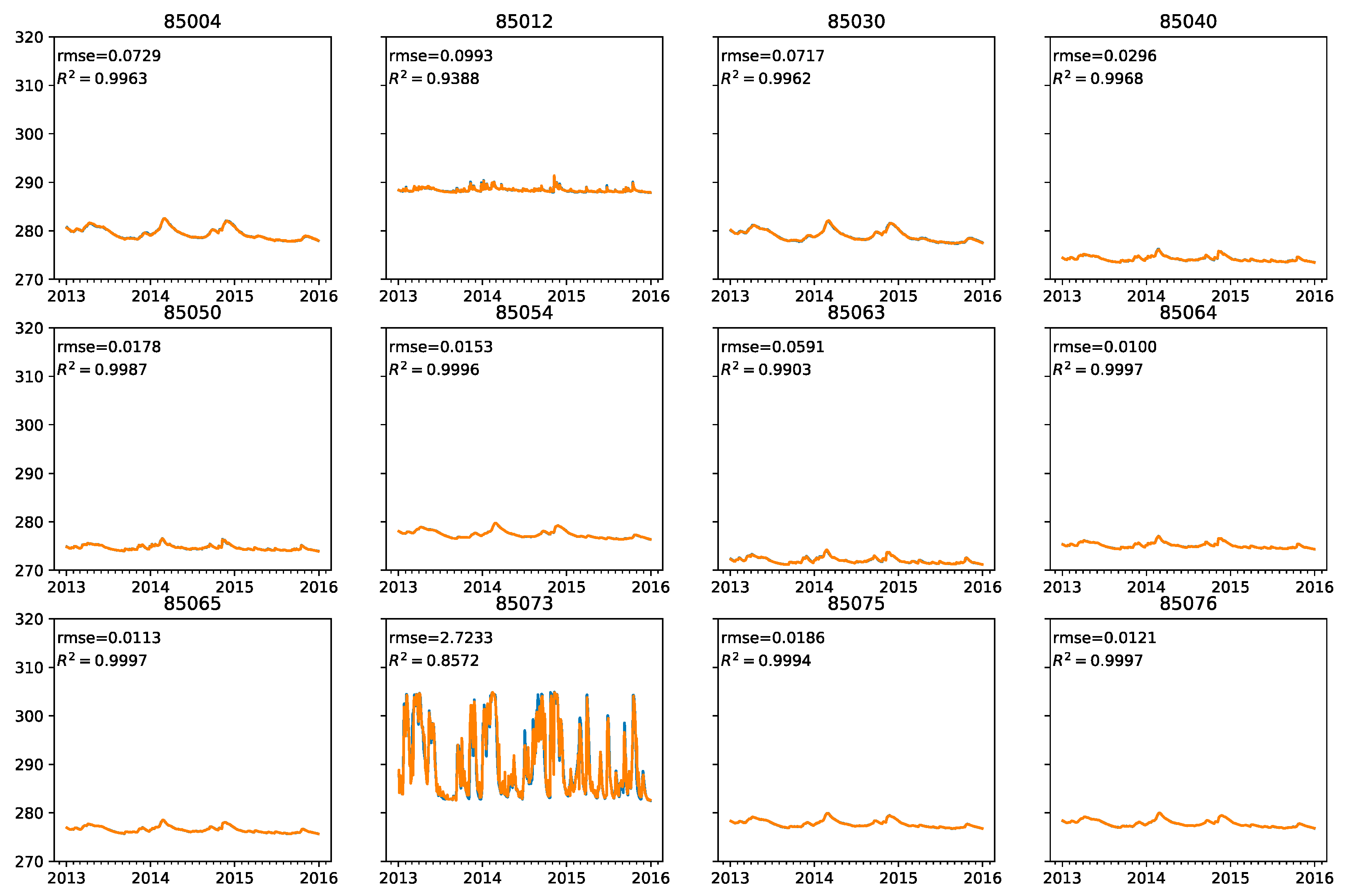
Measurements from each station have been modeled with a combination of measurements from other station (predictors) by linear regression, support vector regressor and random forest regressor. For each station, optimal subset of predictors and modeling algorithm were selected according to R² score (full dataset was split with ratio of 7:3 into train and test set respectively; each model was evaluated on the same test-set).

Results of optimal combinations of predictors and modeling algorithms are presented in

Table 1. Modeling results for different (groups of) sensors.

Sensor	R2	RMSE	Optimal Algorithm	Optimal Predictors
all other	0.9976 (+/−0.0028)	0.0318 (+/−0.0244)	Linear regression	different
85012	0.9388	0.0993	Linear regression	04, 50, 54, 63, 64, 65, 73, 75
85073	0.8572	2.7233	Random forest	04, 30, 50, 54, 63

. First line includes average values of R² and root mean squared error (RMSE; with standard deviation in parenthesis) for 10 similar sensors (last two are presented separately), optimal predictors are not presented, as they vary from station to station (optimal combination includes from 5 to 11 adjacent sensors as predictors). Interestingly, station 85012 (significantly different) is always present as predictor, although its correlation with other sensor is very small. Optimal predictors are presented as last two digits of sensor id, as numbered in Figure 2.

Prediction results of our methodology are extremely good. Highly correlated sensors can be modeled with one another almost perfectly with R² scores are close to 1. On average our algorithm misses by 3 cm. Even the two different sensors (85037 and 85012) have been predicted fairly accurately (R² higher than 0.85), which shows the strength of the data-driven approach. Figure 3 depicts sensor 85067, which has true missing values within our test period.

4. Discussion

Many groundwater sensors within an aquifer are strongly correlated to one another. With a proper usage of data-driven modeling algorithms, feature engineering and optimization procedures we are able to produce extremely accurate estimates for values that are missing. Results with R² close to 1 and RMSE in the range of centimeters show great capabilities of data-driven methods. The obvious shortcoming of these techniques is the demand for existing measurements.

Missing data imputation methodology has been applied to Ljubljana polje aquifer groundwater level data and has proven to be extremely efficient with highly correlated sensors. It was also able to produce adequate results (R² > 0.85) with sensors that are weakly correlated to available predictors. Additional feature engineering is expected to improve the models, which could capture aquifer dynamics better.

5. Conclusions

In this paper we have demonstrated a methodology which transverses the phase space of different regression methods (in our case linear regression, support vector regression, random forest) and all the combinations of corresponding predictors (values of groundwater level from nearby sensors). The methodology is able to select the optimal imputation method for a particular sensor and available set of predictors.

The methodology could be improved with additional feature engineering. Historic values, differences among sensors and differences with historic values could be used to model the underlying processes within the aquifer. Spatial analysis of the available sensor data could be made and domain experts could identify other potentially relevant attributes for groundwater level modeling (surface water properties, weather). The methodology should test the applicability other methods (gradient boosting, neural networks, and different kernels for SVM regression) that internally extend the feature space and can therefore encapsulate the underlying processes in the aquifer in more detail.

Another extension of the methodology could also be for anomaly detection. Since each sensor can be modeled with a set of other sensors, we could cross-validate all the measured values and detect the most obvious outliers. Our methodology uses an ensemble of different prediction methods, which could be used to improve robustness of the outlier detectors. Additionally, our ensembles could provide an estimate of the real value in cases, where the outlier is a consequence of sensor fault.