Biaxial Compression Tests on Hopkinson Bars †

1
LMT, ENS Paris-Saclay/Université Paris-Saclay/CNRS, 94235 Cachan-CEDEX, France
2
CEA Saclay, France
3
UFR Ingénierie, Université Pierre et Marie Curie, Sorbonne Universités, 75005 Paris, France
*
Author to whom correspondence should be addressed.
†
Presented at the 18th European International Conference on Experimental Mechanics (ICEM18), Brussels, Belgium, 1–5 July 2018.
Proceedings 2018, 2(8), 420; https://doi.org/10.3390/ICEM18-05263
Published: 24 May 2018
(This article belongs to the Proceedings of The 18th International Conference on Experimental Mechanics)
Abstract
:A biaxial compression Hopkinson bar set-up bas been designed. It consists in a projectile, an input bar and two co-axial output bars. After the projectile impact on the input bar, the internal output bar measures the axial loading of the cross sample whereas the external output bar measures its transversal loading via a mechanism with sliding surfaces. Gauges glued on the bars enable stain measurements which lead to the forces and to the displacements on the interfaces between the bars and the mounting. The displacement field of the sample is obtained by high-speed imaging and by digital image correlation. Experiments show that the set-up works despites two disadvantages. Firstly, the transversal force in the sample is over-estimated because of the friction in the mechanism. Moreover, comparisons between the displacements on the bars interfaces and the sample displacement field display that the clearance have an influence on the sample loading.
1. Introduction
Multiaxial dynamic loadings usually occur in many industrial cases such as automotive crashes [1]. Researchers have then tried to carry out biaxial compression tests on cross samples by mounting them on Hopkinson bars, which are the most convenient dynamic set-up.
The sample, whose transversal strain is blocked by a rigid device, can be mounted on a compressive Hopkinson bar device [2]. Unfortunately, the ratio between the transversal and the axial stresses strongly depends on the sample material. A preload can be applied on the rigid device, but the obtained load remains quasi-static. Two perpendicular Hopkinson bar devices can be used to generate the biaxial compression state on the sample [3], but obtaining two simultaneous impacts is difficult. Indeed, the projectiles positions should be controlled with an accuracy of a few mm, which implies a quasi-perfect timing of the impacts.
A new set-up has been designed to overcome these difficulties. Tests have been performed and the experimental results are presented in this article.
2. Hopkinson Bar Set-Up and Obtained Measurements
2.1. Set-Up Working and Characteristics
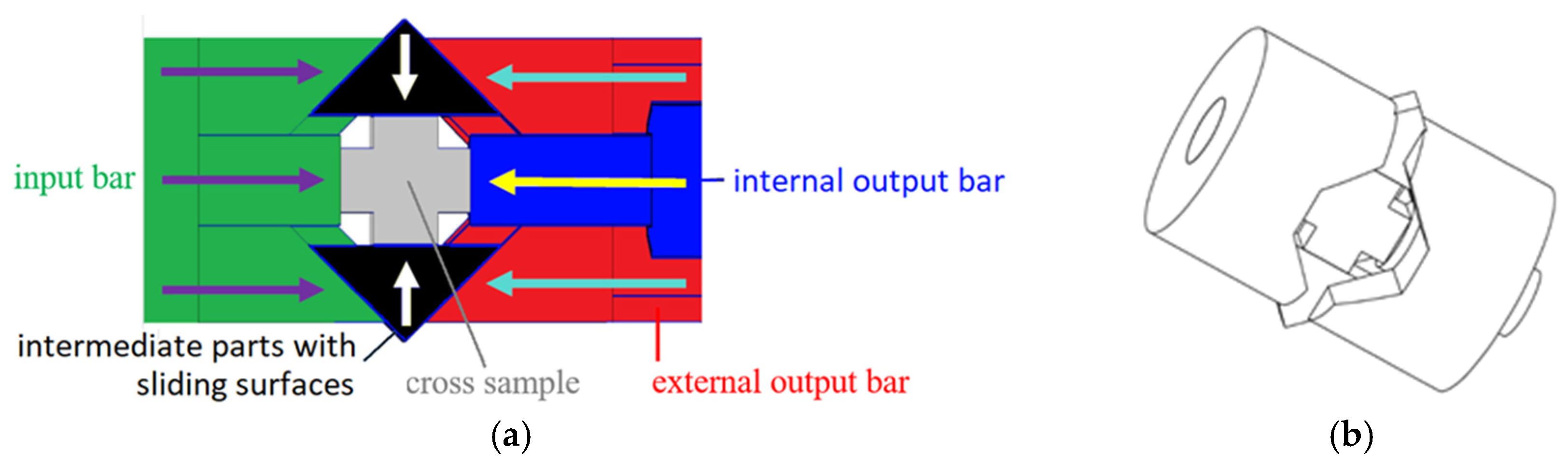
Our new set-up uses a projectile, an input bar and two co-axial output bars (Figure 1). After the projectile impact on the input bar, the internal output bar measures the axial loading of the cross sample whereas the external output bar (a tube surrounding the internal output bar) measures its transversal loading via a mechanism. This mechanism uses two intermediate parts with sliding surfaces at 45° relatively to the axial direction (Figure 1).
Using a single projectile avoids the difficulty due to non-simultaneous impacts occurring with perpendicular Hopkinson bar devices. Another advantage lies in the fact that the ratio between the axial and the transversal loadings is imposed by the ratio between the external and the internal output bars impedances and by the sliding surfaces angle, i.e., by the set-up itself and not by the sample material like with rigid confinements.
The bars are made of steel and their characteristics are given in Table 1. The sample is made of aluminum, its size (boundary to boundary) is 10 mm × 10 mm and its thickness is 5 mm.
2.2. Forces and Velocities Measurements
Axial strain gauges are glued at the middle of the input bar and on the two output bars close to the sample but far enough from the boundaries to be within the Saint-Venant’s conditions (at 612 mm from the interface with the mounting on the internal bar, and at 374 mm on the external bar). Their measurement frequency is 500 kHz.
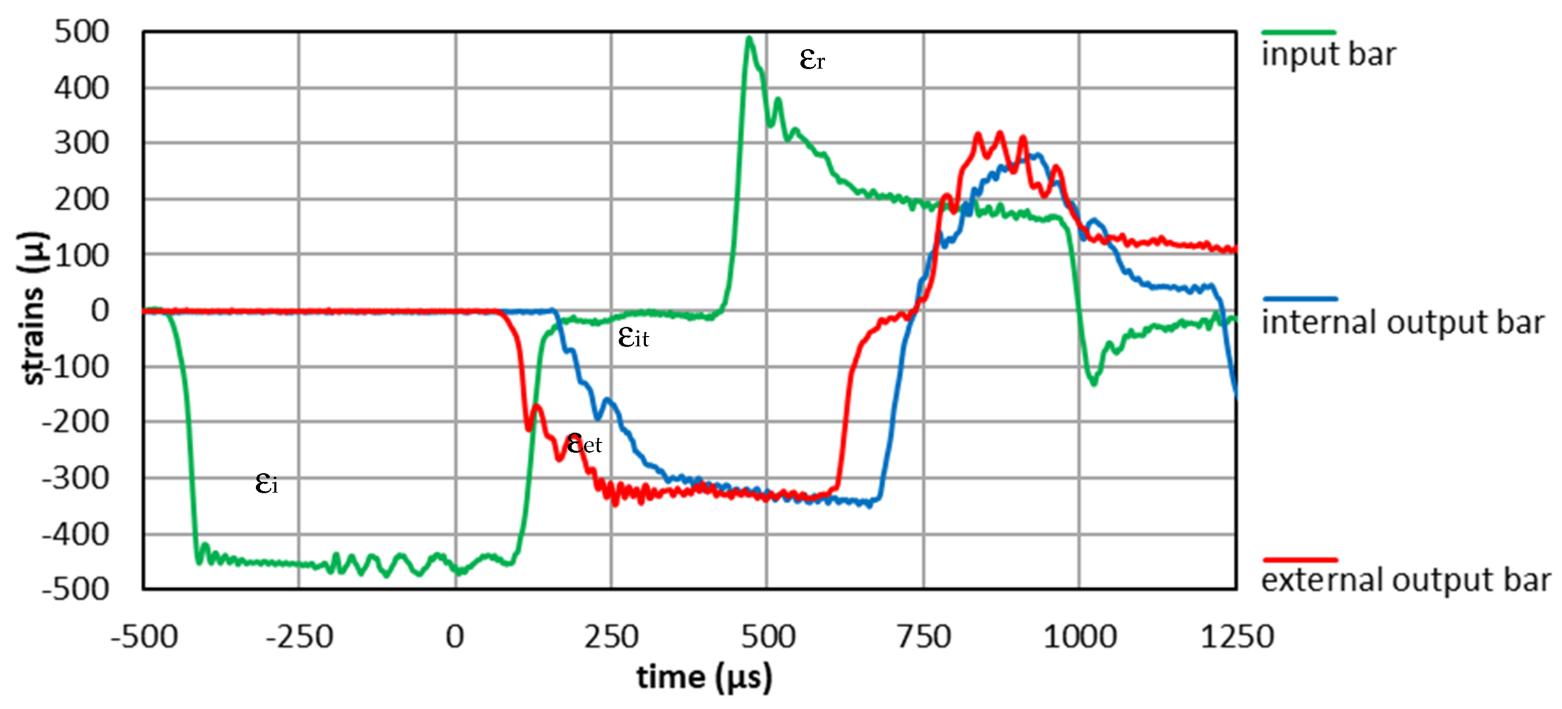
The impact of the striker generates an incident compressive strain wave εi in the input bar. Then, reverberation occurs in the Figure 1 mounting, leading to a reflected strain wave εr in the input bar and to two transmitted compressive waves in the internal and external output bars, respectively denoted εit and εet. The first waves are measured by the gauge glued on the input bar where εi is followed by εr. The transmitted waves εit and εet are respectively measured by the gauge glued on the internal output bar and by the gauge glued on the external output bar (Figure 2).
These strain waves have to be virtually transported from the gauges positions to the interfaces between the bars and the mounting. Thus, εi has to be delayed and εr, εit and εet have to be shifted forward of the duration necessary for the waves to propagate from the measurement gauge to the corresponding boundary. Then the Hopkinson formulae enable the determination of the forces and of the velocities at the interfaces from these transported waves and from the Table 1 parameters:
Fi and Vi being the force and the velocity at the interface between the input bar and the Figure 1 mounting, Fio and Vio the force and the velocity at the interface between the internal output bar and the mounting, and Feo and Veo the force and the velocity at the interface between the external output bar and the mounting.
As it remains in an equilibrium state (see Section 3.1), the axial force in the sample can be supposed to be equal to Fio. Moreover, by neglecting the friction in the mechanism (which is relevant with lubricated surfaces), the transversal force in the sample can be supposed to be equal to Feo.
By neglecting the clearances and the intermediate strains in the mechanism, the axial elongation rate (assumed positive in compression) can be supposed to be equal to the difference between Vi and Vio. Similarly, the transversal elongation rate (positive in compression) can be supposed to be equal to the difference between Vi and Veo. All the corresponding displacements and elongations can be determined by performing a numerical integration based on the rectangle method.
2.3. Images Processing
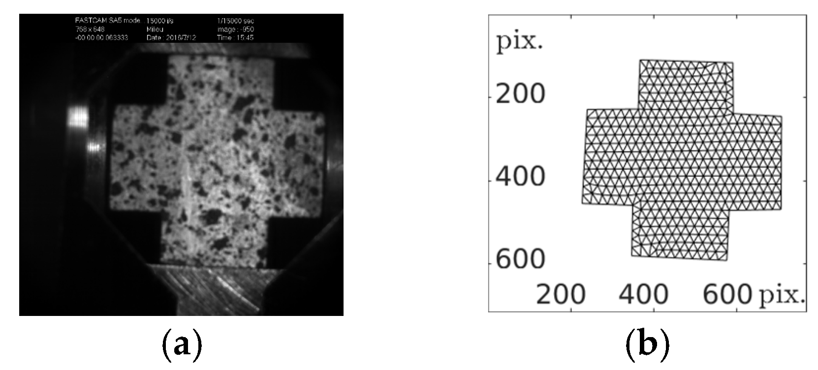
The speckled cross sample is observed thanks to a high-speed camera whose frequency is 15 kHz at a resolution of 768 pix × 648 pix. Images of the sample are obtained during the test. The first one is called the reference image and the displacement field between each image and the reference one is calculated thanks to Digital Image Correlation (DIC) (the displacement field is thus null for the reference image). The reference image is shown on Figure 3.
DIC is performed by using the in-house Correli RT3 software [4]. The displacement field is decomposed over a finite-element mesh composed of triangular 3-noded elements (T3). The chosen element size is 20 pixels, which leads to the mesh presented on Figure 3.
The reference image is numbered 0 and the following images are numbered from 1. The mean displacement on the sample boundaries (left, right, upper and lower) is determined from DIC over a 5-pixel thickness. As shown on Figure 3, the axial displacement is algebraically oriented from left to right and the transversal one is oriented from top to bottom.
In order to control the uncertainty of the DIC calculation, an elastic regularization can be used [4]. The Poisson’s ratio used to perform the regularization is 0.49. Such a magnitude has been chosen to take account of the sample incompressibility in its plastic phase, which will be mainly studied.
The relative weight applied to the reference solution can be seen as the fourth power of a length called the regularization length. The effect of this regularization term is to smoothen the displacement field at small scales (less than the regularization length) so that it comes closer to the solution of the elastic problem with a diffuse boundary condition which results from the DIC problem.
The elastic regularization just helps to obtain a mechanically relevant displacement field and the associated stress field has no physical sense.
3. Experimental Results
3.1. Forces Equilibrium
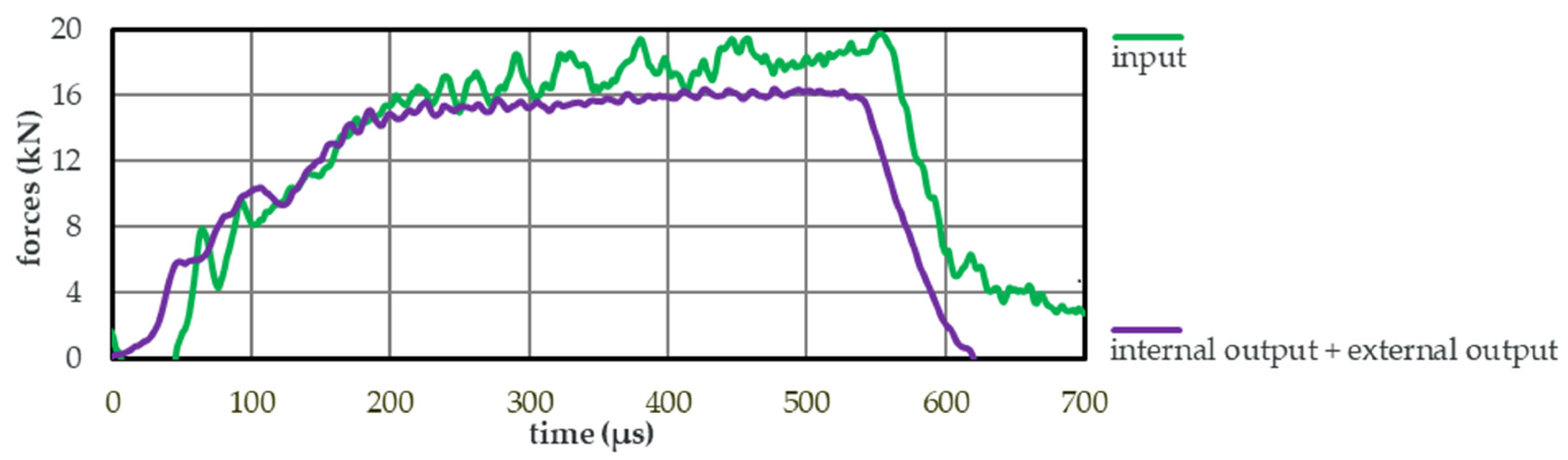
The Hopkinson Formulae (1)–(6) enable the forces determination at the interfaces between the bars and the mounting from the strain gauges measurements. The forces time evolutions can be seen on Figure 4, and one can see a satisfactory equilibrium. This equilibrium implies that the forces in the cross sample can be deduced from the forces at the interfaces as explained in Section 2.2.
3.2. Images Processing
A too high regularization length can lead to erroneous estimations of the experimental displacement field because this field is thus constrained to be closed to an elastic solution. As a result, the DIC calculations are processed with a regularization length decreasing from a value corresponding to 6 times the element size to a value equal to the element size. The regularization influence can therefore be studied and the most relevant length can be selected.
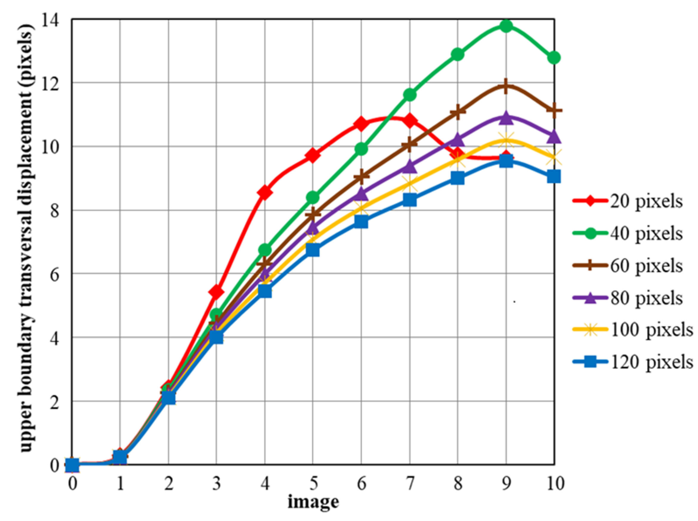
Regularization has a negligible influence on the estimated lower boundary transversal displacement and on the estimated left and right boundaries axial displacements, and a small influence on the estimated upper boundary transversal displacement. One can see on Figure 5 that the dependence is firstly strong from 20 pix to 60 pix and that it decreases after. It can be explained by a noise reduction. As a convergence seems established beyond a 100-pix length, this value is finally chosen. This choice is a compromise between noise reduction and estimated displacements reliability.
3.3. Time Shifting of the Images Relatively to the Gauges Signals
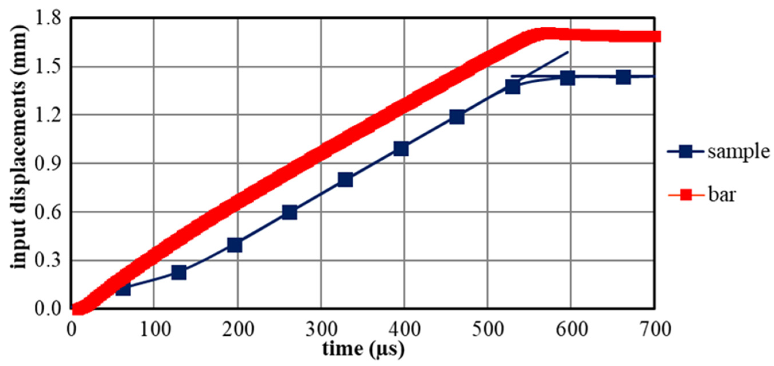
The cross sample has 5 mm-width arms and this width can be estimated to 235 pix on Figure 3. Pix being now converted into mm, the time evolutions of the displacement at the input bar interface (see Section 2.2) and of the displacement at the sample left boundary (see Section 2.3) are compared:
The sample displacement frequency (the camera frequency) is far lower than the bar displacement one (the gauge acquisition one). Because of the clearances, the instants corresponding to the beginning of the loading are not the same on the bar and on the sample. However, the unloading instants can be supposed to be the same. The unloading instant on the sample is supposed to correspond to the intersection between a line determined thanks to a linear regression applied on the loading phase and an horizontal line corresponding to the mean displacement value after loading (Figure 6). The sample displacement and the bar displacement curves are then shifted knowing that the two unloading instants should be the same. The fact that the slopes of the two curves are the same tends to prove the measurements reliability.
3.4. Stress and Strain State Reached during the Test
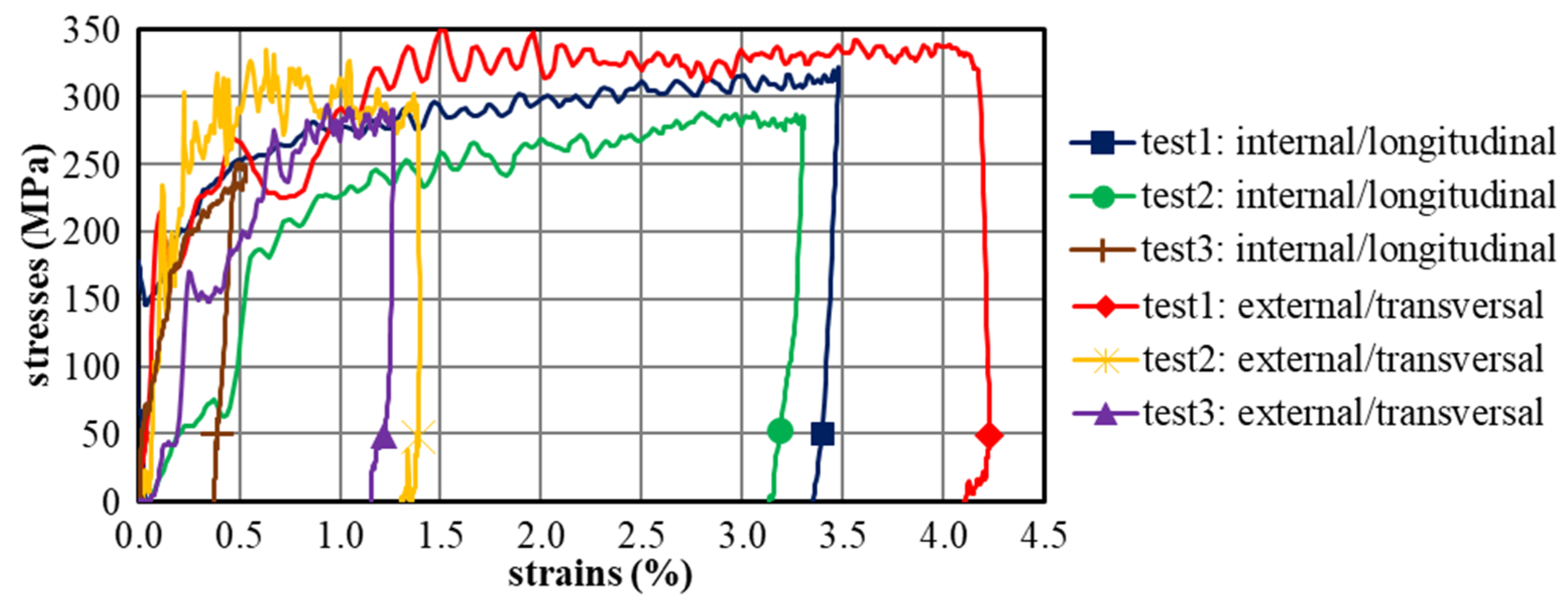
The displacements given by the camera can be obtained at the gauges frequency thanks to polynomial interpolations. The global strains in both directions can be calculated knowing the sample dimensions. Numerical differentiations of their time evolutions lead to strain rates of the order of 100 s−1. The longitudinal stress in the sample is supposed to be equal to the ratio between Fio and the arm section (5 mm × 5 mm), and the transversal stress can be supposed to be equal to the ratio between Feo and the arm section (see explanations in Section 2.2). The stress-strain laws in both directions are given on Figure 7. The curves obtained from the studied test, noted “1”, are compared to those obtained from two other tests (“2” and “3”).
Because of the friction at the sliding surfaces, the transversal force, supposed to be equal to Feo, is over-estimated. Because of the sample isotropic behavior, the two stress perfect-plastic thresholds observed on Figure 7 (clearly exhibited for the “test 1”) should be the same, so one can supposes that the slight difference between the stress levels is due to this over-estimation.
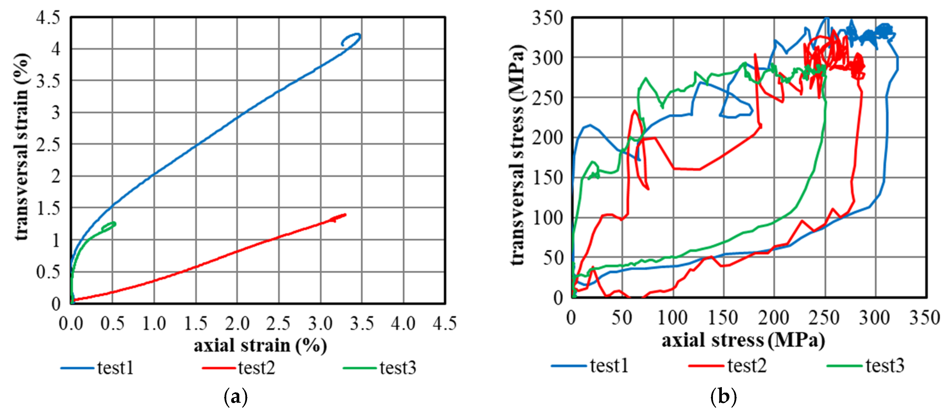
Figure 8 show that the axial and the transversal loadings are not the same. It is caused by the fact that the initial clearances are different between the axial parts of the mechanism than between the transversal ones.
4. Conclusions
A new set-up has been designed and the measurements obtained from a test have been deeply studied. Despites the transversal force over-estimation and the influence of the clearances on the loading, a great challenge has been achieved: the design of an easily buildable set-up generating and measuring a dynamic isotropic biaxial compression loading.
Author Contributions
B.D. conceived and designed the experiments; A.Z. performed the experiments; B.D. and H.Z. analyzed the data and wrote the paper.
Conflicts of Interest
The authors declare no conflict of interest.
References
- Durrenberger, L. Analyse de la Pré-Déformation Plastique sur la Tenue au crash d’une Structure Crash-Box par Approches Expérimentale et Numérique. Ph.D Thesis, Paul Verlaine University of Metz, Metz, France, 2007. [Google Scholar]
- Albertini, C.; Cadoni, E.; Solomos, G. Advances in the Hopkinson bar testing of irradiated/non-irradiated nuclear materials and large specimens. Phil. Trans. R. Soc. A Math. Phys. Eng. Sci. 2014, 372, 2015. [Google Scholar] [CrossRef] [PubMed]
- Carlo Albertini, M.M. Dynamic Uniaxial and Biaxial Stress-Strain Relationships for Austenitic Stainless Steels. Nucl. Eng. Des. 1980, 57, 107–123. [Google Scholar] [CrossRef]
- Tomicevc, Z.; Hild, F.; Roux, S. Mechanics-aided digital image correlation. J. Strain Anal. 2013, 48, 330–343. [Google Scholar] [CrossRef]
Figure 1.
(a) Cut view of the mounting with the relative motion of each part (on scale); (b) Three-dimensional view.
Figure 1.
(a) Cut view of the mounting with the relative motion of each part (on scale); (b) Three-dimensional view.

Figure 2.
Time evolutions of the strains measured by the gauges with the waves εi, εr, εit and εet.

Figure 3.
(a) Reference image; (b) Corresponding mesh on the sample.

Figure 4.
Time evolutions of the input force and of the total output force at the interfaces.

Figure 5.
Upper boundary transversal displacement depending on the regularization length.

Figure 6.
Comparison between the displacements on the input bar interface and on the sample left boundary.
Figure 6.
Comparison between the displacements on the input bar interface and on the sample left boundary.

Figure 7.
Stress depending on strain in both directions.

Figure 8.
(a) Transversal strain as a function of the axial one; (b) Transversal stress as a function of the axial one.
Figure 8.
(a) Transversal strain as a function of the axial one; (b) Transversal stress as a function of the axial one.


Table 1.
Volumetric mass densities, tensile-compressive wave celerities, radii and lengths of the bars.
Table 1.
Volumetric mass densities, tensile-compressive wave celerities, radii and lengths of the bars.
| Bar | Density | Wave Celerity | Radius | Length | |
|---|---|---|---|---|---|
| External | Internal | ||||
| striker | ρi = 8050 kg·m−3 | Ci = 4600 m·s−1 | Ri = 11 mm | 1.25 m | |
| input | 4 m | ||||
| internal output | ρio = 7800 kg·m−3 | Cio = 5100 m·s−1 | Rio = 6 mm | 2 m | |
| external output | ρeo = 7400 kg·m−3 | Ceo = 5200 m·s−1 | Reeo = 11 mm | Rieo = 9 mm | 2 m |
© 2018 by the authors. Licensee MDPI, Basel, Switzerland. This article is an open access article distributed under the terms and conditions of the Creative Commons Attribution (CC BY) license (https://creativecommons.org/licenses/by/4.0/).
Share and Cite
MDPI and ACS Style
Durand, B.; Zouari, A.; Zhao, H. Biaxial Compression Tests on Hopkinson Bars. Proceedings 2018, 2, 420. https://doi.org/10.3390/ICEM18-05263
AMA Style
Durand B, Zouari A, Zhao H. Biaxial Compression Tests on Hopkinson Bars. Proceedings. 2018; 2(8):420. https://doi.org/10.3390/ICEM18-05263
Chicago/Turabian StyleDurand, Bastien, Ahmed Zouari, and Han Zhao. 2018. "Biaxial Compression Tests on Hopkinson Bars" Proceedings 2, no. 8: 420. https://doi.org/10.3390/ICEM18-05263