
Estimation of the Surface Area Covered by Snow and the Resulting Runoff Using Landsat Satellite Images †


School of Surveying and Geospatial Engineering, College of Engineering, University of Tehran, Tehran 1417466191, Iran
*
Author to whom correspondence should be addressed.
†
Presented at the 4th International Electronic Conference on Geosciences, 1–15 December 2022; Available online: https://sciforum.net/event/IECG2022 .
Proceedings 2023, 87(1), 36; https://doi.org/10.3390/IECG2022-13961
Published: 10 January 2023
(This article belongs to the Proceedings of The 4th International Electronic Conference on Geosciences)
Abstract
:Snow is one of the most important sources of water in most parts of the world, supplying approximately a third of the water needed for agricultural activities, drinking, and underground water sources. The runoff caused by melted snow can be destructive, and the high volume of snow can lead to an avalanche; therefore, it is important to estimate it. The area of the snow research is around Goose Lake in California, USA, where the ground snow measuring station is (Latitude: 41.92999, Longitude: −120.4168117). The snow can be measured and calculated using the daily satellite imagery of the Landsat for a period of five years (2017–2022) for approximately four months (December–March) (total of approximately 40 images). The information from ground snow measuring stations was used to evaluate the final results. The accuracy assessment shows 76% accuracy.
1. Introduction
Snow is a mixture of ice crystals and water. Snow covers up to 53% of the Earth’s surface in the Northern Hemisphere and up to 44% of the Earth’s surface in the Southern Hemisphere throughout the year. (The country of the United States of America, which is the region studied in this article, is located in the northern hemisphere) [1]. At least one-third of the water used to irrigate agricultural lands in the world comes from runoff caused by the melting of fallen snow. Today, the effects of snow and the resulting runoff have become more important due to the impact this has on agriculture and its products, in addition to causing floods and avalanches. When it snows, this can freeze agricultural crops and the fertile soil of the region, during which the soil loses its fertility and destroys the agricultural crops. For these reasons, if the amount of snowfall in a region is estimated, and according to algorithms and patterns, the area and the amount of snowfall in the desired area is estimated, it can help farmers in a matter of days and even in the same timeframe. Next year, necessary and preventive measures should be taken to prevent the destruction of agricultural products and soil [2,3].
Snow cover, a significant component of the icy realm known as the cryosphere, holds remarkable influence over Earth’s climate system. It affects the distribution of energy on the surface, impacts the water cycle, influences primary productivity, and even plays a role in the exchange of gases at the surface. Additionally, snow cover serves as a valuable indicator of climate change, as its accumulation and melting patterns closely correlate with temperature variations [4].
Other effects of snow and runoff include floods and avalanches. When it snows, surveyors can estimate the probability of an avalanche by using sensor images taken from that area at certain hours and days and calculating the area and volume of snow. Additionally, by calculating the amount of runoff produced from snow, they can predict the probability and volume of floods. Snow depth can provide quantitative information about snow material and energy. Snow depth measurement methods based on station observations are highly accurate; however, these methods cannot present the spatiotemporal changes in snow depth in the observation stations because the observation stations are often sparse. The ability to access vast databases using remote sensing data has provided a fast and effective way to continuously monitor snow depth in all weather conditions and with high time resolution [5].
In the field of remote sensing, it is assumed that electromagnetic radiation from snow has a direct relationship with the depth of snow. Different methods have been provided to estimate the depth of snow. Tang et al. [6] have developed an algorithm that depends on a linear relationship between snow depth and temperature brightness. This algorithm was improved by various researchers; for example, Foster considered foster and terrain parameters to improve snow depth. Kim et al. [5] used Landsat and MODIS images to estimate snow depth. In their proposed method, several functions were analyzed to investigate the relationship between snow depth and snow cover fraction. The utilization of MODIS (Moderate Resolution Imaging Spectroradiometer) snow cover products has become prevalent in regional snow cover studies and modeling endeavors. These products offer daily, freely accessible data with a global reach, encompassing a medium spatial resolution. Despite their popularity, it’s important to note that certain applications may encounter challenges due to potential cloud cover that can obscure the observations [7,8].
Due to the mentioned reasons, for the continuous and accurate monitoring of the amount of snowfall and the calculation of the resulting runoff, there is a need for satellite images with a not-very-long sensor return period and with high resolution. Additionally, the purpose of using satellite images is to receive and extract information regarding snow parameters; a sensor whose images include thermal bands should be used so that snow-covered areas can be distinguished and extracted from other areas. One of the famous sensors suitable for processing snow-covered images is the Landsat 8 sensor, and its return period is 16 days [9,10,11,12,13,14].
Using the NDSI index and the NDVI index, the normalized index of the difference and changes in snow cover and vegetation, on Landsat sensor images, the snow surface is determined in the photo without cloud cover. The desired image prepared in this project is a satellite image that was taken from the United States of America, the city of California, and near Goose Lake in 4 months (December–March) from 2017 to 2022, and it has snow cover. The image used in this article is from the second series of Landsat sensor products (which are in the form of 16-day periods).
2. Data and Study Area
2.1. Study Area
Goose Lake region in latitude 41.92999 and longitude −120.4168117 has been selected as the study area (Figure 1). The time selected for this study is from 2017 to 2022. This region is located at latitude 41.92999; as a result, it is a region that is considered one of the cold regions and, due to weather conditions, snow cover is seen in this region.
2.2. Data
This study used remotely sensed and in situ datasets. Remotely sensed data comprise Landsat8-TM (spatial resolution 30 m), acquired from 2017 to 2022, obtained through the google earth engine platform. Table 1 shows additional information on the remotely sensed dataset.
3. Methodology
The conceptual model of the proposed method is presented according to the flowchart in Figure 3.
In this method, first, Landsat images related to December, January, February, and March of 2017 to 2022, which had less than 10% cloud cover, were downloaded. Then, their NDSI images were calculated according to the following equation:
In this equation, Green band and SWIR band, respectively, correspond to bands 3 and 6 of Landsat 8 image. NDSI measures the relative value of the reflectance difference between the Green and SWIR bands and controls the variance between the two bands, which is useful for the field of snow mapping. Snow is not reflective only in the visible range, and it also has high absorption in NIR or SWIR. This parameter is considerably helpful in separating between clouds and snow. Another parameter used in this study to estimate snow depth is NDVI. NDVI is an index sensitive to vegetation and due to the existence of vegetation in the region, it can be important for separating snowy areas.
The NDVI index is calculated according to the following equation:
In this equation, the NIR band and R band, respectively, correspond to bands 4 and 5 of Landsat 8 image. According to the calculated NDSI and NDVI images of two regions for different times, SCF was produced by the formula presented in the article “Mapping Snow Depth Using Moderate Resolution Imaging Spectroradiometer Satellite Images: Application to the Republic of Korea”, which combines NDVI and NDSI to build a snow cover map [15,16].
After calculating SCF, the relationship between snow depth and SCF is estimated. According to the studies, the relationship between snow depth and SCF is an exponential relationship or linear form; therefore, it is necessary to investigate an exponential function and linear function for this purpose according to Formulas (4)–(6).
Snow Depth = a × (SCF) + b
Snow Depth = a × exp (b × SCF)
Snow Depth = a × exp (b × SCF) + c × exp (d × SCF)
To calculate the a, b, c, d unknown parameters of Equations (4)–(6), equivalent values of ground stations are used. The 30 pieces of information related to three stations were used to calculate the coefficients α and β and the information about the station and 50 other pieces of information about stations were used to evaluate the accuracy. For accuracy evaluation, the RMSE parameter is used, which provides the difference between the values at the station and the calculated values.
In the next step, to calculate snow depth, SCF, NDSI and NDVI were applied to estimate equivalent snow water in the study area. A multi-layer perceptron was applied to create a relationship between the aforementioned parameters. Figure 3 shows a schematic presentation of the proposed method. A multilayer perceptron is a fully connected class of feedforward artificial neural networks. If a multilayer perceptron has a linear activation function in all neurons, that is, a linear function that maps the weighted inputs to the output of each neuron, then linear algebra shows that any number of layers can be reduced to a two-layer input–output model. Learning occurs in the perceptron by changing connection weights after each piece of data is processed, based on the amount of error in the output compared to the expected result.
4. Results
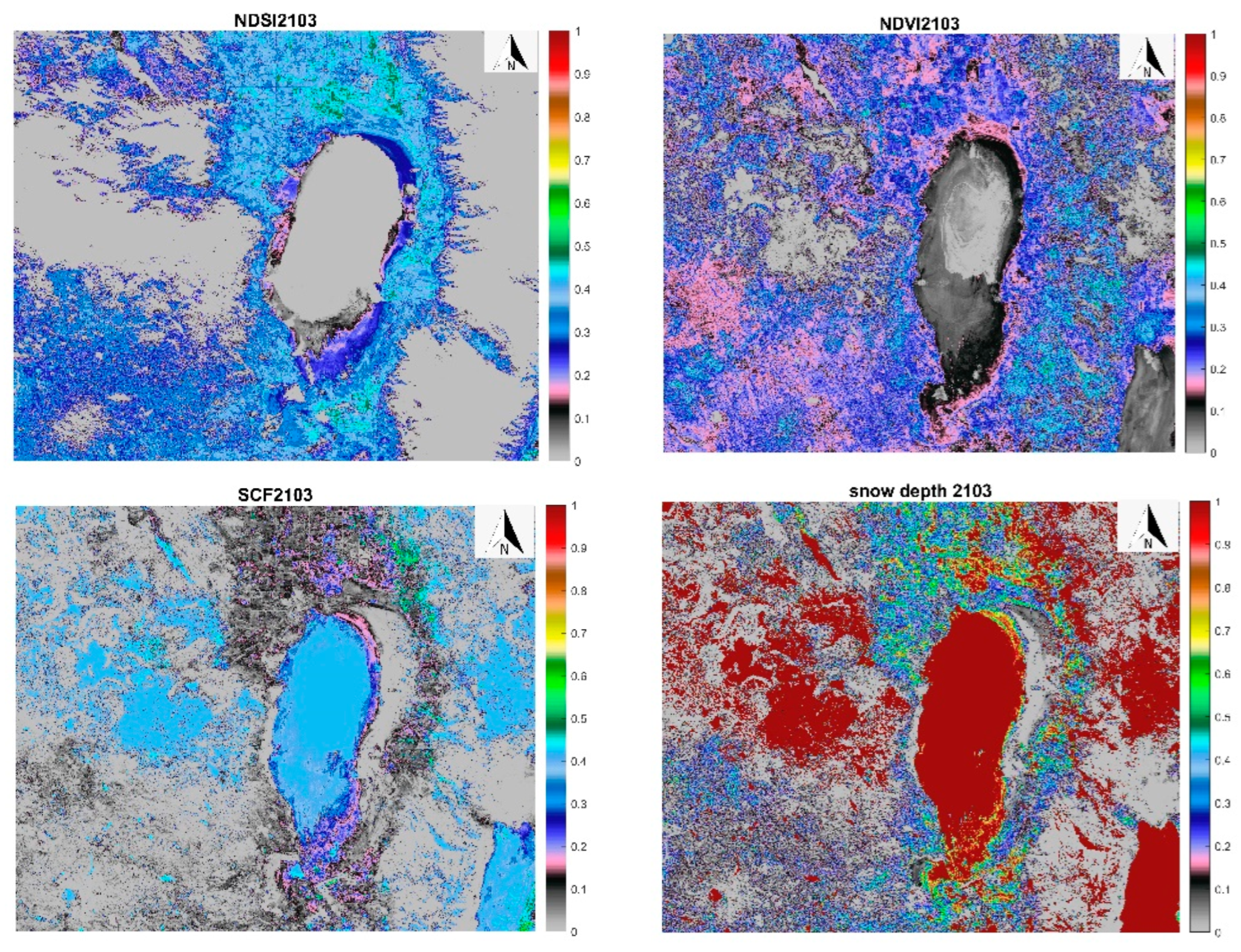
According to the proposed method, the outputs of NDVI, NDSI, SCF and snow depth related to March of 2021 are shown in Figure 4.
Table 3 shows some of the training data in order to clarify the estimation problem. In this Table, snow depth in situ data provided are from the USDA website and considered as a reference criterion to calculate accurate equation models related to calculated snow cover fraction (Equations (4)–(6)).
Based on the investigation, the linear and exponential relationship between in situ snow depth and calculated snow cover fraction (figure) was calculated using 30 corresponding data, and the value of a, b, c and d is estimated using the least squares method. Equations (7)–(9) indicate the estimated formulas for linear, first-order exponential function and second-order exponential function, respectively.
Snow depth = a × (SCF) + b
a = 5.426
b = −0.0113
a = 5.426
b = −0.0113
Snow Depth = a × exp (b × SCF)
Coefficients (with 95% confidence bounds):
a = 0.3699 (0.2377, 0.5021)
b = 4.159 (3.364, 4.953)
Coefficients (with 95% confidence bounds):
a = 0.3699 (0.2377, 0.5021)
b = 4.159 (3.364, 4.953)
Snow Depth = a × exp (b × SCF) + c × exp (d × SCF)
Coefficients (with 95% confidence bounds):
a = −6.95 (−6.95, −6.95)
b = −4.326 × 10⁻⁶ (−1.9 × 10⁻⁵, 1.035 × 10⁻⁵)
c = 6.95 (6.95, 6.95)
d = 0.67 (0.67, 0.67)
Coefficients (with 95% confidence bounds):
a = −6.95 (−6.95, −6.95)
b = −4.326 × 10⁻⁶ (−1.9 × 10⁻⁵, 1.035 × 10⁻⁵)
c = 6.95 (6.95, 6.95)
d = 0.67 (0.67, 0.67)
In order to evaluate the estimated parameters of 50 in situ snow depth data, the corresponding snow cover fraction was used to calculate root mean square error (RMSE). According to the result the RMSE for linear function is equal to 0.0166 m, which is an acceptable value. The RMSE for first-order exponential function (Equation (8)) is equal 0.2502 m. Additionally, the RMSE for second-order exponential function is equal to 1.86 × 10⁻⁸ m.
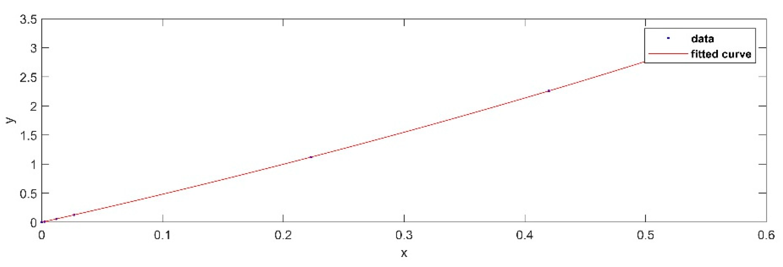
According to the results, the second-order exponential function provides a better result compared to the linear and first-order exponential functions. Figure 5 shows the fitness of the second-order exponential function on the input data. The figure also shows the optimized curve for exponential fits based on the current dataset.
After calculating snow depth, an artificial neural network with three layers (input, hidden and o output layer) was defined to estimate the equivalent water (snow depth water). The input layer includes four neurons (NDVI, SCF, NDSI, Snow Depth), the hidden layer includes three neurons and the output layer includes one neuron that corresponded to the equivalent snow water. Sigmoid function was set as the activation function and different learning rate, epoch number and hidden layer ‘s neurons tested the sensitivity analysis of the proposed network. According to the results, the RMSE was equal to 0.32069, 0.309, 0.3918, 0.27, 0.273, 0.543, 0.257, 0.251 m for the 0.3, 0.6, 0.1, 0.7, 0.8, 0.01, 0.9, 0.95 learning rates, respectively. According to the results, the learning rate set equal to 0.95 show better results. In the next step, the epoch numbers were tested to select the optimum epoch numbers. The RMSE was equal to 0.246, 0.246, 0.245, 0.247 m for 4, 6, 10, 20 epoch numbers, respectively. The results show stability against different epoch numbers. When the neurons of hidden layer are set to 1, the RMSE is equal to 0.247 m; if the neurons equal 2, the RMSE is 0.243; and if the neurons equal 3, the RMSE is 0.242 m. The results are stable for the number of neurons in the hidden layer and the number of epochs.
5. Conclusions
The paper proposed the snow depth parameter calculation based on the snow cover faction parameter. Snow cover fraction was calculated using NDVI and NDSI index. According to the results, the second-order exponential function shows the best fitness between calculated snow depth and ground station snow depth. The equivalent water (run off) can be estimated based on NDVI, NDSI, SCF and snow depth parameters. The artificial neural network is considered a powerful method to investigate the relationship between these parameters.
Author Contributions
Conceptualization, K.K., R.S.-H. and S.K.; methodology, software, validation, formal analysis, investigation, resources, data curation, writing—original draft preparation, writing—review and editing visualization, K.K., R.S.-H. and S.K.; supervision R.S.-H. All authors have read and agreed to the published version of the manuscript.
Funding
This research received no external funding.
Institutional Review Board Statement
Not applicable.
Informed Consent Statement
Not applicable.
Data Availability Statement
No new data were created.
Conflicts of Interest
The authors declare no conflict of interest.
References
- Kim, D.; Jung, H.-S. Mapping Snow Depth Using Moderate Resolution Imaging Spectroradiometer Satellite Images: Application to the Republic of Korea. Korean J. Remote Sens. 2018, 34, 625–638. [Google Scholar]
- Tong, R.; Parajka, J.; Komma, J.; Blöschl, G. Mapping snow cover from daily Collection 6 MODIS products over Austria. J. Hydrol. 2020, 590, 125548. [Google Scholar] [CrossRef]
- Guo, J.; Jiao, Z.; Cui, L.; Yin, S.; Chang, Y.; Xie, R.; Li, S.; Zhu, Z. A Method to Identify High-Quality Pure Snow Data in Polder Database. In Proceedings of the IGARSS 2020-2020 IEEE International Geoscience and Remote Sensing Symposium, Waikoloa, HI, USA, 26 September–2 October 2020. [Google Scholar]
- Dong, C. Remote sensing, hydrological modeling and in situ observations in snow cover research: A review. J. Hydrol. 2018, 561, 573–583. [Google Scholar] [CrossRef]
- Kim, D.; Jung, H.-S.; Kim, J.-C. Comparison of snow cover fraction functions to estimate snow depth of South Korea from MODIS imagery. Korean J. Remote Sens. 2017, 33, 401–410. [Google Scholar]
- Tang, Y.; Zhang, W.; Liu, L.; Li, G. Spring thaw classification based on AMSR-E brightness temperature in the central Tibetan Plateau. Int. J. Remote Sens. 2019, 40, 6542–6552. [Google Scholar] [CrossRef]
- Gao, Y.; Xie, H.; Yao, T.; Xue, C. Integrated assessment on multi-temporal and multi-sensor combi-nations for reducing cloud obscuration of MODIS snow cover products of the Pacific Northwest USA. Remote Sens. Environ. 2010, 114, 1662–1675. [Google Scholar] [CrossRef]
- Hall, D.K.; Riggs, G.A.; DiGirolamo, N.E.; Román, M.O. Evaluation of MODIS and VIIRS cloud-gap-filled snow-cover products for production of an Earth science data record. Hydrol. Earth Syst. Sci. 2019, 23, 5227–5241. [Google Scholar] [CrossRef]
- Romanov, P.; Tarpley, D. Enhanced algorithm for estimating snow depth from geostationary satellites. Remote Sens. Environ. 2007, 108, 97–110. [Google Scholar] [CrossRef]
- Salomonson, V.V.; Appel, I. Development of the Aqua MODIS NDSI fractional snow cover algorithm and validation results. IEEE Trans. Geosci. Remote Sens. 2006, 44, 1747–1756. [Google Scholar] [CrossRef]
- Lin, J.; Feng, X.; Xiao, P.; Li, H.; Wang, J.; Li, Y. Comparison of snow indexes in estimating snow cover fraction in a mountainous area in northwestern China. IEEE Geosci. Remote Sens. Lett. 2012, 9, 725–729. [Google Scholar]
- Roy, A.; Royer, A.; Turcotte, R. Improvement of springtime stream-flow simulations in a boreal environment by incorporating snow-covered area derived from remote sensing data. J. Hydrol. 2010, 390, 35–44. [Google Scholar] [CrossRef]
- Ault, T.W.; Czajkowski, K.P.; Benko, T.; Coss, J.; Struble, J.; Spongberg, A.; Templin, M.; Gross, C. Validation of the MODIS snow product and cloud mask using student and NWS cooperative station observations in the Lower Great Lakes Region. Remote Sens. Environ. 2006, 105, 341–353. [Google Scholar] [CrossRef]
- Da Ronco, P.; Avanzi, F.; De Michele, C.; Notarnicola, C.; Schaefli, B. Comparing MODIS snow products Collection 5 with Collection 6 over Italian Central Apennines. Int. J. Remote Sens. 2020, 41, 4174–4205. [Google Scholar] [CrossRef]
- Grayson, R.; Blöschl, G. (Eds.) Spatial Patterns in Catchment Hydrology: Observations and Modelling; CUP Archive: Cambridge, UK, 2001. [Google Scholar]
- Hall, D.K.; Riggs, G.A. Normalized-Difference Snow Index (NDSI); Singh, V.P., Singh, P., Haritashya, U.K., Eds.; Encyclopedia of Snow, Ice and Glaciers; Springer: Dordrecht, The Netherlands, 2011; pp. 779–780. [Google Scholar] [CrossRef]
Figure 1.
Goose Lake map.

Figure 2.
Ground station distribution map from USDA website (https://www.nrcs.usda.gov/).
Figure 2.
Ground station distribution map from USDA website (https://www.nrcs.usda.gov/).

Figure 3.
Detailed work flowchart in developing the snow depth map from Landsat images.

Figure 4.
NDSI, NDVI, SCF, snow depth images from March 2021.

Figure 5.
The second-order exponential curve fitted on the current dataset.


Table 1.
Satellite data description.
| Satellite | Acquired Time from-to |
|---|---|
| Landsat8/TM | From 12/2017 to 03/2022 |
Table 2.
In situ dataset description.
| Station Name | Lat/long | Time |
|---|---|---|
| Crowder Flat | 41.89/−120.75 | From 12/2017 to 03/2022 |
| Dismal Swamp | 41.99/−120.18 | From 12/2017 to 03/2022 |
| State Line | 41.99/−120.72 | From 12/2017 to 03/2022 |
| Strawberry | 42.13/−120.84 | From 12/2017 to 03/2022 |
Table 3.
The example of some training data to compute relationship between snow depth and SCF.
| Station Id | Station Name | NDVI | NDSI | Latitude | Longitude | Snow Depth (In Situ) | SCF (Calculated) |
|---|---|---|---|---|---|---|---|
| 977 | Crowder Flat | 0.5274 | −0.587 | 41.89 | −120.75 | 2.75 × 10⁻⁵ | 5.91 × 10⁻⁶ |
| 977 | Crowder Flat | 0.06 | −0.477 | 41.89 | −120.75 | 2.258635 | 0.42 |
| 977 | Crowder Flat | 0 | −013 | 41.89 | −120.75 | 2.258635 | 0.42 |
| 446 | Dismal swamp | 0.26 | −0.771 | 41.99 | −120.18 | 2.05 × 10⁻⁵ | 4.40 × 10⁻⁶ |
| 446 | Dismal swamp | 0.195 | −0.327 | 41.99 | −120.18 | 0.010533 | 0.00226 |
| 446 | Dismal swamp | 0.258 | −0.015 | 41.99 | −120.18 | 6.42 × 10⁻⁵ | 1.38× 10⁻⁵ |
Disclaimer/Publisher’s Note: The statements, opinions and data contained in all publications are solely those of the individual author(s) and contributor(s) and not of MDPI and/or the editor(s). MDPI and/or the editor(s) disclaim responsibility for any injury to people or property resulting from any ideas, methods, instructions or products referred to in the content. |
© 2023 by the authors. Licensee MDPI, Basel, Switzerland. This article is an open access article distributed under the terms and conditions of the Creative Commons Attribution (CC BY) license (https://creativecommons.org/licenses/by/4.0/).
Share and Cite
MDPI and ACS Style
Kazari, K.; Shah-Hosseini, R.; Khanbani, S. Estimation of the Surface Area Covered by Snow and the Resulting Runoff Using Landsat Satellite Images. Proceedings 2023, 87, 36. https://doi.org/10.3390/IECG2022-13961
AMA Style
Kazari K, Shah-Hosseini R, Khanbani S. Estimation of the Surface Area Covered by Snow and the Resulting Runoff Using Landsat Satellite Images. Proceedings. 2023; 87(1):36. https://doi.org/10.3390/IECG2022-13961
Chicago/Turabian StyleKazari, Kiana, Reza Shah-Hosseini, and Sara Khanbani. 2023. "Estimation of the Surface Area Covered by Snow and the Resulting Runoff Using Landsat Satellite Images" Proceedings 87, no. 1: 36. https://doi.org/10.3390/IECG2022-13961