The Influence of Antarctic Sea Ice Distribution on the Southern Ocean Overturning Circulation for the Past 20,000 Years ^†

Abstract

Changes in Southern Ocean physics are dynamically linked to westerly winds, ocean currents, and the distribution of Antarctic sea ice in the Southern Hemisphere. As a result, it is critical to comprehend the response of Southern Ocean physics to the distribution of Antarctic sea ice on a basin scale. This modeling study employs a fully coupled Earth system model to investigate the effect of Antarctic Sea ice distribution on Southern Ocean dynamics during the past 20,000 years. The findings show that the formation and melting of sea ice have an effect on the distribution of surface buoyancy flux over the Southern Ocean. The simulated sea ice edge (grid points in the ice model have a sea ice concentration above 5%) in the Southern Ocean almost demarcates the borderline between the lower and upper meridional overturning cells. The seemingly permanent Antarctic sea ice edge (grid points in the ice model with a sea ice concentration greater than 80%) coincides with the shift of buoyancy flux from positive (buoyancy gain) to negative (buoyancy loss). Furthermore, the negative surface buoyancy flux zone has shifted polewards for the past 20,000 years, with the exception of approximately 14.1 thousand years. Our findings show that Antarctic sea ice feedback affects the surface buoyancy flux, affecting the overturning circulation in the Southern Ocean.

1. Introduction

Studies have advocated that the Southern Ocean atmosphere, Antarctic sea ice, and ocean are dynamically interconnected [1,2]. For example, ocean–sea ice feedback involves melting summertime sea ice, which brings liquid freshwater back to the ocean. Additionally, the formation of wintertime sea ice (brine rejection) brings salt content to the ocean surface. Thus, Antarctic sea ice regulates freshwater flux by melting summertime sea ice and salt flux by wintertime brine rejection.

Numerous studies have found that the alteration in Southern Hemisphere westerly winds, Antarctic sea ice change, and accompanying surface buoyancy fluxes play a fundamental part in altering atmospheric carbon dioxide concentrations on orbital timescales by modulating the Southern Ocean deep ocean stratification and overturning circulation [1,3,4,5,6,7,8]. The understanding of Southern Ocean dynamics is currently developing. The paleoclimatology community recognizes that the Southern Ocean overturning circulation is primarily driven by wind [9,10]. However, several studies have found that changes in buoyancy flux caused by freshwater discharge [11,12], ocean eddies [13], topography [12], and Antarctic sea ice feedback [1,4,14,15,16,17] contributed to Southern Ocean dynamical changes during the most recent deglacial period. As a result, it is critical to comprehend the role of Antarctic sea ice in surface buoyancy flux, which influences the Southern Ocean overturning circulation.

Buoyancy flux is the density change across the air–sea interface initiated by heating/cooling and evaporation/precipitation. Positive buoyancy flux (buoyancy gain) indicates areas with lower surface ocean density. Furthermore, the area with higher surface ocean density is represented by negative buoyancy flux (buoyancy loss). Cold temperatures limit seawater thermal expansion at high latitudes in the Southern Ocean [18]. For that reason, freshwater changes dominate Southern Ocean surface buoyancy [19] related to summertime sea ice melting [11,20]. Buoyancy gain from sea ice melting would help transform the deep returning flow into the Southern Ocean’s intermediate and mode waters [21].

However, wintertime formation of Southern Ocean sea ice and associated brine rejection contribute to buoyancy loss around Antarctica [22,23]. Buoyancy loss from Southern Ocean surface cooling and sea ice growth encourage bottom water formation into ocean basins. Recent research has shown that alterations in the extent of Antarctic sea ice cause a change in surface buoyancy, thus modulating the Southern Ocean overturning circulation [1,3,13,14,24].

Therefore, focusing on Antarctic sea ice change is essential to understand the ocean’s role in regulating atmospheric carbon dioxide concentrations on glacial–interglacial time scales. Previous studies have shown that the melting of Antarctic sea ice releases freshwater, which increases the buoyancy of Southern Ocean upwelled water [25] and strengthens the upper limb of the ocean meridional overturning circulation [11,26]. Furthermore, numerical simulations have confirmed the importance of freshwater fluxes in determining changes in Southern Ocean upwelling during the last deglacial period [8,14,15].

Southern Ocean sea ice coverage significantly boosts deep ocean carbon sequestration by reducing the exposure time of surface waters with the atmosphere and minimizing the vertical mixing of deep ocean waters, leading to deep ocean stratification [1,17]. The presence of Antarctic sea ice decreases momentum exchange from air to the surface of the Southern Ocean while also reducing air–sea gas exchange, which increases deep ocean carbon sequestration [27]. Furthermore, model-based and satellite data studies have also highlighted the critical role of Antarctic sea ice in future and present climate scenarios. Recent climate-induced variability in the extent of seasonal Antarctic sea ice has been shown to influence thermohaline circulation and marine primary production [28]. Therefore, focusing on and comprehending the significance of Antarctic sea ice distribution over the last 20 K (K refers to 1000 years before the present) will assist us in comprehending current and future changes in Southern Ocean dynamics.

2. Materials and Methods

This study uses a general circulation model that includes the ocean, atmosphere, ice, and land surfaces referred to as the TraCE-21ka experiment [29]. A T31_gx3v5 resolution version of the Community Climate System Model (CCSM3) from the National Center for Atmospheric Research (NCAR) is included in the experiment. The modeling experiment uses the Community Atmosphere Model version 3 (CAM3), Community Sea Ice Model version 5 (CSIM5), Parallel Ocean Program version (POP), and Community Land Surface Model version 3 (CLM3). The boundary conditions for the climate model include transient variations in the meltwater fluxes in the Northern and Southern Hemispheres, incoming solar radiation, retreating continental ice sheet topography, which is indicated by the rise in eustatic sea level, and atmospheric greenhouse gas concentrations. The model output data are accessible to the public at https://www.earthsystemgrid.org/project/trace.html (most recent access was on 27 October 2022).

The atmospheric model for the experiment uses the Community Atmospheric Model 3 (CAM3), which is run at a T31 resolution (about 3.75 degrees) and at 26 hybrid vertical coordinate levels. The resolutions of the experiment output data from the Parallel Ocean Program (POP) and NCAR Community Sea Ice Model version 5 (CSIM5) are comparable (gx3v5). The ocean and ice output data contain 3.6 degrees of longitudinal resolution and varying degrees of latitudinal resolution, making them around 0.9 degrees close to the equator. As a result, the output data from the ocean and ice models are interpolated to a resolution of 3.75 degrees. The POP model contains a vertical z coordinate with 25 depth levels and ocean eddies parameterization [30]. The CSIM5 model also includes a distribution of ice thickness on a subgrid-scale.

This study examines the variation of Antarctic sea ice coverage and surface buoyancy flux over the past 20,000 years. The results are shown at 20 K to 19 K (Last Glacial Maximum), 17.3 K to 16.3 K (Heinrich 1 event), 12.5 K to 11.5 K (Younger Dryas event), 11 K to 10 K (onset of the Holocene), 6 K to 5 K, and 2 K to 1 K periods to cover changes during the past 20,000 years.

3. Results and Discussion

We analyzed ocean and sea ice data to understand the Antarctic sea ice distribution feedback on surface ocean properties over the past 20,000 years.

This study defines the seemingly permanent sea ice–ocean edge as the Southern Ocean surface area covered with sea ice most of the year. We calculated the seemingly permanent sea ice–ocean edge as grid points in the ice model which have a sea ice concentration above 80 percent. Figure 1 highlights the near superimposition between the seemingly permanent sea ice–ocean edge marked in blue and the borderline between positive to negative surface buoyancy fluxes shown by the solid black line from the 20 K to 19 K to 11 K to 10 K period. This implies that the simulated Southern Ocean surface area covered by Antarctic sea ice for the majority of the year overlaps with the buoyancy loss zone (densification). Further analysis shows that in both the Indian and Pacific Ocean sectors, the latitudinal position of the buoyancy flux transition zone shifts poleward by approximately 11° from the 20 K to 10 K period.

Specifically, the superimposition was better during the 11 K to 10 K period in the Indian and Pacific Ocean sectors. On the other hand, the seemingly permanent sea ice–ocean edge was displaced equatorward in the Atlantic Ocean sector. This is because of the equatorward transport of sea ice from the Weddell Sea gyre. Moreover, the demarcation between the positive and negative buoyancy fluxes also displaced equatorward in the Atlantic Ocean sector. However, the buoyancy flux transition zone did not overlap with the seemingly permanent sea ice edge, unlike the Indian and Pacific Ocean sectors.

The 17.3 K to 16.3 K and 12.5 K to 11.5 K periods represent Northern Hemisphere cooling and, therefore, Southern Hemisphere warming periods (bipolar seesaw) [31]. Figure 2 shows the overlapping between the seemingly permanent sea ice–ocean edge and the borderline between the positive and negative buoyancy fluxes similar to the 11 K to 10 K periods. This shows the association of sea ice with surface buoyancy flux in the Southern Ocean during Southern Hemisphere warm events. Additionally, the inference stands true in the 6 K to 5 K and 2 K to 1 K periods, highlighting the association of sea ice with surface buoyancy fluxes throughout the past 20,000 years.

Southern Ocean studies have shown that water draws from deeper ocean layers along inclined outcropping density surfaces poleward of the Antarctic polar front [10]. The rising of warmer deep water melts ice in the open ocean and on the shelf and, therefore, controls the northern extent of the Southern Ocean cryosphere. Studies have found that the 1027.6 ${\mathrm{kg} \mathrm{m}}^{-3}$ isopycnals outcrop coincides with the winter ice edge. Therefore, the density surface of 1027.6 ${\mathrm{kg} \mathrm{m}}^{-3}$ isopycnals roughly demarcates the division between the upper and lower meridional overturning cells [22].

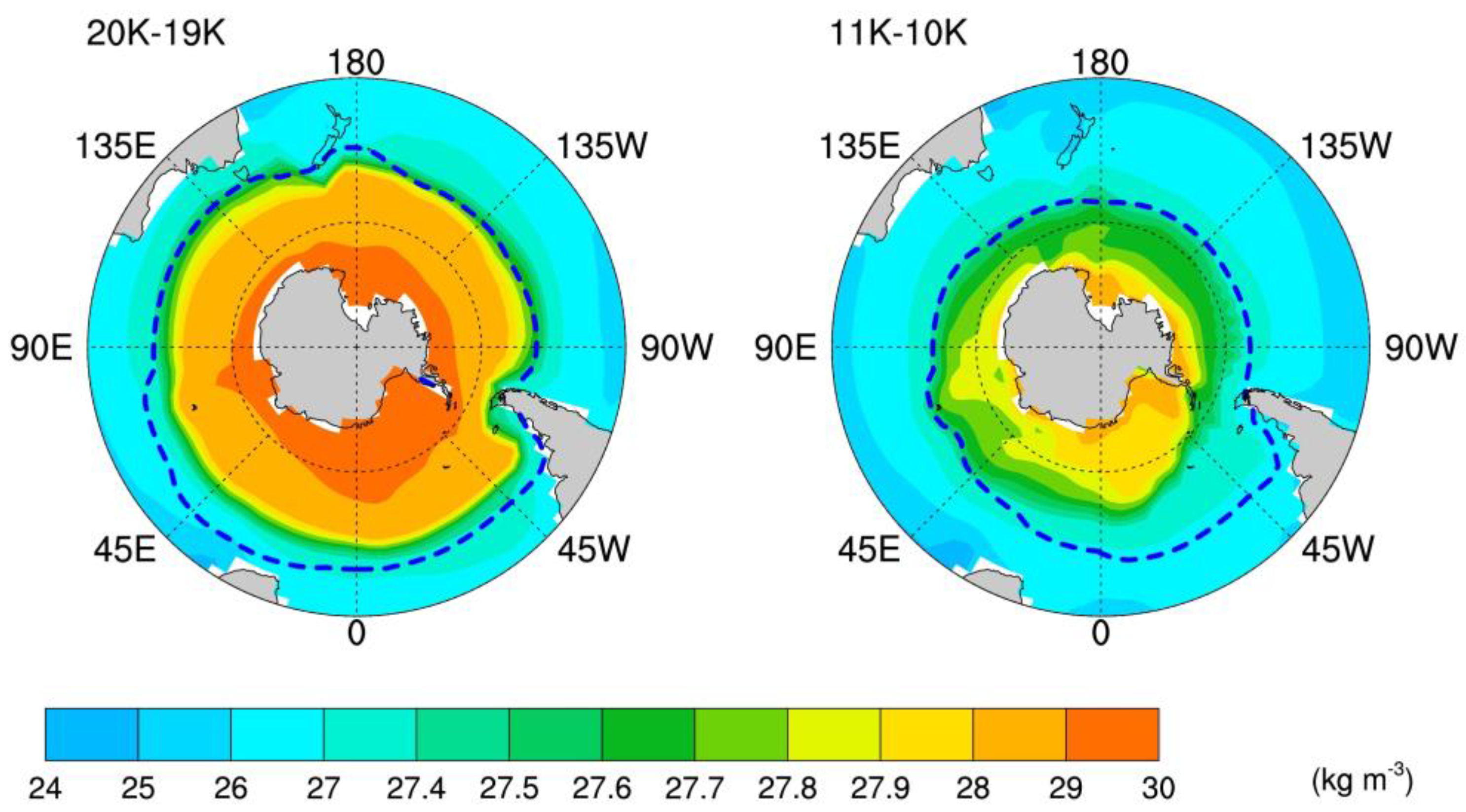
Grid points in the ice model with a sea ice concentration of more than five percent were considered the Antarctic sea ice–ocean border in this study. Figure 3 shows that the distribution of Southern Ocean surface waters varies during the deglacial period. The Southern Ocean’s denser surface waters were expanded equatorward during the 20 K to 19 K period compared to the 11 K to 10 K period. Figure 3 highlights that the Antarctic sea–ocean edge reasonably overlaps with ocean surface density between 1027.5 to 1027.7 ${\mathrm{kg} \mathrm{m}}^{-3}$ in the Indian and Pacific Ocean sectors. Therefore, the Antarctic sea ice edge coarsely demarcates the division between the upper and lower meridional overturning cells throughout the most recent deglacial period in the Pacific and Indian Ocean sectors. However, this association is not shown in the Atlantic Ocean sector.

During the 17.3 K to 16.3 K and 12.5 K to 11.5 K Southern Hemisphere warming periods, Figure 4 shows the overlapping between the seemingly permanent sea ice–ocean edge and the borderline between the positive and negative buoyancy fluxes similar to the 11 K to 10 K period. This shows the association of sea ice with surface buoyancy flux in the Southern Ocean during Southern Hemisphere warm events. Additionally, the inference stands true in the 6 K to 5 K and 2 K to 1 K periods, highlighting the association of sea ice with surface buoyancy fluxes throughout the past 20,000 years.

The Allerød warm phase (14 K to 12.9 K) was brought on by the meltwater pulse 1A (mwp-1A) event, which the model experiment predicted occurred at around 14.1 K [29]. During the mwp-1A event, the model experiment implemented both Southern (Antarctic) and Northern Hemisphere meltwater forcings. The meltwater forcing in the Southern was three times more than in the Northern Hemisphere and was included in the ocean model as a freshwater flux onto the surface ocean in the Weddell Sea (Atlantic Ocean) region, as indicated by surface freshening in Figure 5. Therefore, the 14.1 K event characterizes the response of freshwater freshening on the surface Southern Ocean in the Atlantic Ocean sector.

Figure 5 shows the near superimposition between the seemingly permanent sea ice–ocean edge and the borderline between the negative and positive buoyancy fluxes in the Indian and Pacific Ocean sectors but does not follow in the Atlantic Ocean sector, which is similar throughout the last deglacial period. Additionally, the surface ocean is anomalously fresh near the Antarctic continent in the Atlantic Ocean (Weddell Sea) and Pacific Ocean sectors in response to surface freshwater forcing. The sea ice edge also overlaps with ocean surface density between 1027.5 to 1027.7 ${\mathrm{kg} \mathrm{m}}^{-3}$ in the Indian and Pacific Ocean sectors, but does not follow in the Atlantic Ocean sectors.

4. Conclusions

This study investigated the association of Antarctic sea ice distribution on the Southern Ocean surface density and associated buoyancy flux employing the TraCE-21ka model experiment. The seemingly permanent sea ice coverage overlays with the buoyancy loss zone over the Southern Ocean during the past 22,000 years. Consequently, an alteration in the Antarctic sea ice distribution would alter the surface buoyancy flux coverage. Moreover, the Southern Ocean surface area, which is covered with sea ice most of the year, regulates the Southern Ocean circulation by demarcating the borderline between the upper (Atlantic Meridional Ocean Circulation) and lower meridional overturning circulation.

This study emphasizes the importance of studying Antarctic sea ice distribution to understand the coupling of atmosphere-ocean–sea ice at high latitudes. It also highlights the association between Antarctic sea ice coverage, surface buoyancy forcing, and the Southern Ocean overturning circulation. This relationship is critical in future climate modeling studies in order to recognize the changes in the Southern Ocean overturning circulation and their climate implications. Therefore, this research may aid in understanding the natural global warming process and its impacts on the dynamics of the Southern Ocean.

References

- Abernathey, R.P.; Cerovecki, I.; Holland, P.R.; Newsom, E.; Mazloff, M.; Talley, L.D. Water-mass transformation by sea ice in the upper branch of the Southern Ocean overturning. Nat. Geosci. 2016, 9, 596–601. [Google Scholar] [CrossRef]
- Anderson, R.F.; Ali, S.; Bradtmiller, L.I.; Nielsen, S.H.H.; Fleisher, M.Q.; Anderson, B.E.; Burckle, L.H. Wind-Driven Upwelling in the Southern Ocean and the Deglacial Rise in Atmospheric CO2. Science 2009, 323, 1443–1448. [Google Scholar] [CrossRef] [PubMed]
- Cerovečki, I.; Talley, L.D.; Mazloff, M.R. A Comparison of Southern Ocean Air–Sea Buoyancy Flux from an Ocean State Estimate with Five Other Products. J. Clim. 2011, 24, 6283–6306. [Google Scholar] [CrossRef]
- Chen, C.; Wang, G. Simulated Southern Ocean Upwelling at the Last Glacial Maximum and Early Deglaciation: The Role of Eddy-Induced Overturning Circulation. Geophys. Res. Lett. 2021, 48, e2021GL092880. [Google Scholar] [CrossRef]
- Ferrari, R.; Jansen, M.F.; Adkins, J.F.; Burke, A.; Stewart, A.L.; Thompson, A.F. Antarctic sea ice control on ocean circulation in present and glacial climates. Proc. Natl. Acad. Sci. USA 2014, 111, 8753–8758. [Google Scholar] [CrossRef]
- Fischer, H.; Schmitt, J.; Lüthi, D.; Stocker, T.F.; Tschumi, T.; Parekh, P.; Joos, F.; Köhler, P.; Völker, C.; Gersonde, R.; et al. The role of Southern Ocean processes in orbital and millennial CO2 variations—A synthesis. Quat. Sci. Rev. 2010, 29, 193–205. [Google Scholar] [CrossRef]
- Gent, P.R.; McWilliams, J.C. Isopycnal Mixing in Ocean Circulation Models. J. Phys. Oceanogr. 1990, 20, 150–155. [Google Scholar] [CrossRef]
- Iudicone, D.; Madec, G.; Blanke, B.; Speich, S. The Role of Southern Ocean Surface Forcings and Mixing in the Global Conveyor. J. Phys. Oceanogr. 2008, 38, 1377–1400. [Google Scholar] [CrossRef]
- Jansen, M.F. Glacial ocean circulation and stratification explained by reduced atmospheric temperature. Proc. Natl. Acad. Sci. USA 2017, 114, 45–50. [Google Scholar] [CrossRef]
- Jansen, M.F.; Nadeau, L.-P. The Effect of Southern Ocean Surface Buoyancy Loss on the Deep-Ocean Circulation and Stratification. J. Phys. Oceanogr. 2016, 46, 3455–3470. [Google Scholar] [CrossRef]
- Karstensen, J.; Lorbacher, K. A practical indicator for surface ocean heat and freshwater buoyancy fluxes and its application to the NCEP reanalysis data. Tellus A Dyn. Meteorol. Oceanogr. 2011, 63, 338–347. [Google Scholar] [CrossRef]
- Lauderdale, J.M.; Williams, R.G.; Munday, D.R.; Marshall, D.P. The impact of Southern Ocean residual upwelling on atmospheric CO2 on centennial and millennial timescales. Clim. Dyn. 2017, 48, 1611–1631. [Google Scholar] [CrossRef]
- Liu, W.; Liu, Z.; Li, S. The Driving Mechanisms on Southern Ocean Upwelling Change during the Last Deglaciation. Geosciences 2021, 11, 266. [Google Scholar] [CrossRef]
- Liu, Z.; Otto-Bliesner, B.L.; He, F.; Brady, E.C.; Tomas, R.; Clark, P.U.; Carlson, A.E.; Lynch-Stieglitz, J.; Curry, W.; Brook, E.; et al. Transient simulation of last deglaciation with a new mechanism for Bolling-Allerod warming. Science 2009, 325, 310–314. [Google Scholar] [CrossRef] [PubMed]
- Lund, D.C.; Chase, Z.; Kohfeld, K.E.; Wilson, E.A. Tracking Southern Ocean Sea Ice Extent With Winter Water: A New Method Based on the Oxygen Isotopic Signature of Foraminifera. Paleoceanogr. 2021, 36, e2020PA004095. [Google Scholar] [CrossRef]
- Mandal, G.; Lee, S.-Y.; Yu, J.-Y. The Roles of Wind and Sea Ice in Driving the Deglacial Change in the Southern Ocean Upwelling: A Modeling Study. Sustainability 2021, 13, 353. [Google Scholar] [CrossRef]
- Mandal, G.; Yu, J.-Y.; Lee, S.-Y. The Roles of Orbital and Meltwater Climate Forcings on the Southern Ocean Dynamics during the Last Deglaciation. Sustainability 2022, 14, 2927. [Google Scholar] [CrossRef]
- Marshall, J.; Speer, K. Closure of the meridional overturning circulation through Southern Ocean upwelling. Nat. Geosci. 2012, 5, 171–180. [Google Scholar] [CrossRef]
- Marzocchi, A.; Jansen, M.F. Connecting Antarctic sea ice to deep-ocean circulation in modern and glacial climate simulations. Geophys. Res. Lett. 2017, 44, 6286–6295. [Google Scholar] [CrossRef]
- Marzocchi, A.; Jansen, M.F. Global cooling linked to increased glacial carbon storage via changes in Antarctic sea ice. Nat. Geosci. 2019, 12, 1001–1005. [Google Scholar] [CrossRef]
- Menviel, L.; Spence, P.; Yu, J.; Chamberlain, M.A.; Matear, R.J.; Meissner, K.J.; England, M.H. Southern Hemisphere westerlies as a driver of the early deglacial atmospheric CO2 rise. Nat. Commun. 2018, 9, 2503. [Google Scholar] [CrossRef] [PubMed]
- Meredith, M.; Sommerkorn, M.; Cassotta, S.; Derksen, C.; Ekaykin, A.; Hollowed, A.; Kofinas, G.; Mackintosh, A.; Melbourne-Thomas, J.; Muelbert, M.M.C.; et al. Polar Regions. In IPCC Special Report on the Ocean and Cryosphere in a Changing Climate; Pörtner, H.-O., Roberts, D.C., Masson-Delmotte, V., Zhai, P., Tignor, M., Poloczanska, E., Mintenbeck, K., Alegri, A., Nicolai, M., Okem, A., et al., Eds.; Cambridge University Press: Cambridge, UK, 2019; in press. [Google Scholar]
- Morrison, A.K.; Frölicher, T.L.; Sarmiento, J.L. Upwelling in the Southern Ocean. Phys. Today 2015, 68, 27–32. [Google Scholar] [CrossRef]
- Morrison, A.K.; Hogg, A.M.; Ward, M.L. Sensitivity of the Southern Ocean overturning circulation to surface buoyancy forcing. Geophys. Res. Lett. 2011, 38, L14602. [Google Scholar] [CrossRef]
- Nadeau, L.-P.; Ferrari, R.; Jansen, M.F. Antarctic Sea Ice Control on the Depth of North Atlantic Deep Water. J. Clim. 2019, 32, 2537–2551. [Google Scholar] [CrossRef]
- Saenko, O.A.; Schmittner, A.; Weaver, A.J. On the Role of Wind-Driven Sea Ice Motion on Ocean Ventilation. J. Phys. Oceanogr. 2002, 32, 3376–3395. [Google Scholar] [CrossRef]
- Skinner, L.C.; Waelbroeck, C.; Scrivner, A.E.; Fallon, S.J. Radiocarbon evidence for alternating northern and southern sources of ventilation of the deep Atlantic carbon pool during the last deglaciation. Proc. Natl. Acad. Sci. USA 2014, 111, 5480–5484. [Google Scholar] [CrossRef]
- Stein, K.; Timmermann, A.; Kwon, E.Y.; Friedrich, T. Timing and magnitude of Southern Ocean sea ice/carbon cycle feedbacks. Proc. Natl. Acad. Sci. USA 2020, 117, 4498–4504. [Google Scholar] [CrossRef]
- Stephens, B.B.; Keeling, R.F. The influence of Antarctic sea ice on glacial–interglacial CO2 variations. Nature 2000, 404, 171–174. [Google Scholar] [CrossRef]
- Talley, L. Closure of the Global Overturning Circulation Through the Indian, Pacific, and Southern Oceans: Schematics and Transports. Oceanography 2013, 26, 80–97. [Google Scholar] [CrossRef]
- Watson, A.; Vallis, G.K.; Nikurashin, M. Southern Ocean buoyancy forcing of ocean ventilation and glacial atmospheric CO2. Nat. Geosci. 2015, 8, 861–864. [Google Scholar] [CrossRef]
Figure 1.
The Southern Hemisphere’s seemingly permanent sea ice coverage (blue color-shaded; fractional concentration) overlaps with the zone of surface buoyancy loss (black–shaded pattern) during the 20 K to 19 K and 11 K to 10 K periods.
Figure 2.
The Southern Hemisphere seemingly permanent sea ice coverage (shaded in blue color; units are in a fraction) overlying the buoyancy loss zone (black shaded pattern) during the 17.3 K to 16.3 K, 12.5 K to 11.5 K, 6 K to 5 K, and 2 K to 1 K periods.
Figure 3.
The density of the ocean’s surface is shown in color-shaded in kilogram per cubic meters units. The ocean surface density data are deduced by 1000, resulting in an ocean surface density of 27.6 for a theoretical ocean surface density of 1027.6 . The surface ocean density is overlaid on the annual mean sea ice–ocean edge (blue dashed line) during the 20 K to 19 K and 11 K to 10 K periods.
Figure 4.
The density of the ocean’s surface is color-shaded in kilogram per cubic meter () units. The surface ocean density is overlaid on the annual mean sea ice–ocean edge (blue dashed line) during the 17.3 K to 16.3 K, 12.5 K to 11.5 K, 6 K to 5 K, and 2 K to 1 K periods.
Figure 5.
The Southern Hemisphere’s seemingly permanent sea ice coverage (blue dashed line) overlays surface ocean density (color-shaded in kilogram per cubic meters ()). Additionally, the buoyancy loss zone (black shaded pattern) overlays the Antarctic’s seemingly permanent sea ice coverage (shaded in blue color; units are in a fraction).
Disclaimer/Publisher’s Note: The statements, opinions and data contained in all publications are solely those of the individual author(s) and contributor(s) and not of MDPI and/or the editor(s). MDPI and/or the editor(s) disclaim responsibility for any injury to people or property resulting from any ideas, methods, instructions or products referred to in the content. |
© 2023 by the authors. Licensee MDPI, Basel, Switzerland. This article is an open access article distributed under the terms and conditions of the Creative Commons Attribution (CC BY) license (https://creativecommons.org/licenses/by/4.0/).
Share and Cite
MDPI and ACS Style
Mandal, G.; Yu, J.-Y.; Lee, S.-Y. The Influence of Antarctic Sea Ice Distribution on the Southern Ocean Overturning Circulation for the Past 20,000 Years. Proceedings 2023, 87, 9. https://doi.org/10.3390/IECG2022-14145
AMA Style
Mandal G, Yu J-Y, Lee S-Y. The Influence of Antarctic Sea Ice Distribution on the Southern Ocean Overturning Circulation for the Past 20,000 Years. Proceedings. 2023; 87(1):9. https://doi.org/10.3390/IECG2022-14145
Chicago/Turabian StyleMandal, Gagan, Jia-Yuh Yu, and Shih-Yu Lee. 2023. "The Influence of Antarctic Sea Ice Distribution on the Southern Ocean Overturning Circulation for the Past 20,000 Years" Proceedings 87, no. 1: 9. https://doi.org/10.3390/IECG2022-14145