UAS-GEOBIA Approach to Sapling Identification in Jack Pine Barrens after Fire


1
Geography, Environment, and Spatial Science, Michigan State University, East Lansing, MI 48824, USA
2
Aviation and Transportation Technology, Purdue University, West Lafayette, IN 47907, USA
*
Author to whom correspondence should be addressed.
Drones 2018, 2(4), 40; https://doi.org/10.3390/drones2040040
Submission received: 30 August 2018
/
Revised: 13 November 2018
/
Accepted: 14 November 2018
/
Published: 21 November 2018
Abstract
:Jack pine (pinus banksiana) forests are unique ecosystems controlled by wildfire. Understanding the traits of revegetation after wildfire is important for sustainable forest management, as these forests not only provide economic resources, but also are home to specialized species, like the Kirtland Warbler (Setophaga kirtlandii). Individual tree detection of jack pine saplings after fire events can provide information about an environment’s recovery. Traditional satellite and manned aerial sensors lack the flexibility and spatial resolution required for identifying saplings in early post-fire analysis. Here we evaluated the use of unmanned aerial systems and geographic object-based image analysis for jack pine sapling identification in a region burned during the 2012 Duck Lake Fire in the Upper Peninsula of Michigan. Results of this study indicate that sapling identification accuracies can top 90%, and that accuracy improves with the inclusion of red and near infrared spectral bands. Results also indicated that late season imagery performed best when discriminating between young (<5 years) jack pines and herbaceous ground cover in these environments.
1. Introduction
Post-fire remote sensing applications aim to provide timely spatial and spectral information regarding forest structure, composition, and vigor during regeneration [1]. Moderate resolution satellite imagery does not provide optimal spatial resolution for individual tree detection (IDT), or in cases where high-spatial resolution is available, and may be costly [2]. Satellite remote sensing also suffers from a lack of flexibility in temporal resolution and is susceptible to atmospheric noise [3]. In contrast, aerial remote sensing provides flight planning that is more flexible and provides increased spatial resolution, but still suffers from atmospheric interference. Given these critical issues, unmanned aerial systems, hereafter referred to as UAS, have gained interest by forest ecologists for understanding patterns, processes, and forest structures [4].
Unmanned aerial systems provide an excellent alternative to satellite imagery, providing higher spatial resolution and temporal frequency at a much more cost-effective rate than manned aircraft and satellite sensors [2,5]. Limitations to their use include small payload capacity, limited battery life, and a lack of professional standards for their use [2,5]. There is a critical need to establish standard protocols to produce reproducible, repeatable workflows. Individual tree detection (IDT) is one application of UAS that is imperative for forest management [6,7].
Several methods exist for ITD using remotely sensed data, many use 3D data, like Light Detection and Ranging (LiDAR). New methods of generating structural data have arisen like structure from motion (SfM). Using UAS imagery to generate SfM multi-view stereo (MVS) is now widely recognized as a valid and low-cost method to generate both orthomosaics and digital surface models (DSMs) derived from 2D image sequences [5,6]. In their study of SfM derived IDT, Reference [7] performed ITD using UAS-SfM derived canopy height models based on algorithms designed for LiDAR data processing. The authors achieved the most accurate results for smoothing window size (SWS) at 3 × 3 irrespective of the fixed window size (FWS). In their assessment of models utilizing SWS and FWS of 3 × 3, the authors achieved a statistical F-scores greater than 0.80. Reference [8] reconstructed poplar saplings using digital photographs and terrestrial LiDAR (T-LiDAR), finding that T-LiDAR was more accurate at 3D construction than digital photographs, but at a much higher cost. Reference [9] examined the potential contribution hyperspectral imagery makes to IDT, achieving accuracies between 40% and 95% in tree detection. A comparison of LiDAR and SfM technology by Reference [10] indicated achieved accuracies of 96% and 80%, respectively, and the authors concluded that the technologies were capable of producing equally acceptable results for plot level estimates. These studies indicate that photogrammetric methods can provide accurate results for identifying tree crowns; however, none of these studies addressed sapling identification in natural environments. Additionally, processing photogrammetric datasets like SfM and LiDAR are computationally intensive for large areas. Finally, Reference [11] developed a land cover classification using multi-view data using a conditional random field (CRF) model, leading to accuracy improvements between 6% and 16.4% for a variety of classification methods. While these methods show promise of integrating multiple image view points for constructing classifications, we posit that there is still a need to develop robust low-cost (computationally and fiscally) methods for IDT; furthermore, there is a need to assess our ability to identify saplings in natural environments using these methods.
An alternative to structure-based methods of IDT is spectral analysis. Near infrared (NIR) and red (R) spectral brightness values can provide important indictors regarding vegetation. Green leaves exhibit maximum chlorophyll absorption at 0.69 µm (red) and show optimal reflection in the adjacent near-infrared region (0.85 µm) [12]. The reflectance values in these two regions are exploited in a number of vegetation indices such as the Normalized Difference Vegetation Index (NDVI) [13]. The NDVI is used for a wide range of applications including land cover classification, deforestation, change detection, and monitoring [14]. It also serves as an indicator of biophysical parameters, like leaf-area index (LAI), biomass, and absorbed photosynthetically active radiation (fAPAR) [15]. Using the ratio method, NDVI reduces noise due to cloud shadowing, atmospheric attenuation, and illumination differences [16]. The NDVI has several shortcomings as well, including oversaturation of signal in high-biomass regions and background sensitivity [17].
More recently, multispectral sensors aboard remote sensing platforms have begun to include a red-edge (RE) band, a sensor recording reflectance of the segment of the electromagnetic spectrum between the R and NIR bands. One such sensor is the MicaSense RedEdge 3, that includes an RE Band ranging from 0.701 µm and 0.724 µm. Similarly, the Rapid-Eye multispectral imager acquires RE data between 0.69 µm and 0.73 µm [14]. These RE sensors are sensitive chlorine and nitrogen concentrations [18,19,20], land cover classification [18], and to improve detection of damage to tree foliation [21]. Given the relative novelty of these sensors, there is some debate about how much they can improve accuracy achievable with combinations of the R and NIR bands.
This paper is also motivated by broader ecological and management objectives. Jack pine ecosystems, like those across Northern Michigan, are particularly influenced by fire [22]. Modern fire rotation in Michigan’s jack pine forests have extended an order of magnitude longer than historical fire rotations [22]. Forest fire suppression due to human settlement has led to a decrease in the extent of jack pine ecosystems within the state [23]. Understanding disturbance regimes within these forests is important for the assessment and design of management practices, like natural disturbance emulation [24]. Earlier research suggests that burned sites lead to greater species richness than clear-cut sites, which may affect species of interest, like the endangered Kirtland Warbler (Setophaga kirtlandii) [25]. To understand more clearly how fire regimes affect early regeneration of jack pine ecosystems, timely, high-resolution data are needed.
According to Reference [26] there is still limited understanding of how UAS data are acquired, processed, and used. The aim of this research is to understand the spectral and seasonal requirements necessary for ITD of jack pine (Pinus banksiana) saplings in a post-fire environment through the use of multispectral imagery. We evaluate (1) which spectral band combinations provide the best accuracy in the detection of jack pine saplings and (2) which period in the vegetation growing season is the most suitable to properly identify jack pine saplings.
2. Methods and Materials
2.1. Study Area
Started on 23 May 2012, the Duck Lake Fire scorched nearly 8900 ha of forest north of Newberry, Michigan (46°39’20.84” N, 85°26’11.59” W). The Michigan Department of Natural Resources (MDNR) manages the site, located in the Lake Superior National Forest. A subsection of the fire-affected area was used in this analysis, as shown in Figure 1.
The sandy nature of soils in this area are likely the result of being covered by Glacial Lake Algonquin, which extended over much of the Eastern Upper Peninsula circa 11,000 B before present (BP). This glacial lake deposited a wide variety of sediment from the sands found around Seney, Michigan to the south west of the study site to heavy clay in Chippewa County, to the east of the study site [27]. This study area is characterized by having sandy, well-drained soils [28] with reduced nutrient content.
The Upper Peninsula of Michigan is categorized as having a humid continental climate. The highest average temperature occurs during the month of July at 78 °F (25.7 °C). The lowest average temperature during the year occurs in January at 24 °F (−4.5 °C). August and September have the highest average precipitation at 3.5 inches per month; February is the driest month on average with only 1.18 inches of precipitation. There is a fair amount of cold weather with temperatures below freezing, leading to a change in precipitation from rain to snow. This usually occurs in late November or early December when the average temperature drops below freezing at 29 °F (−1.8 °C). Snow usually continues until March when the average temperature returns to the mid-30s (37 °F, 2.5 °C).
The vegetation cover is characterized by a mixture of coniferous and deciduous tree species such as white spruce (Picea glauca), jack pine (Pinus banksiana), balsam fir (Abies balsamea), Black spruce (Picea mariana), tamarack (Larix laricina), maple (Acer), hemlock (Tsuga), American beech (Fagus grandifolia), white birch (Betula papyrifera), and aspen (Populus tremuloides) [29]. The landscape is characterized by sparse woody vegetation, framed by older unburned stands as shown in Figure 2. Stand density and age varies across the study area; however, both study sites used here were burned in the 2012 fire.
2.2. UAS Image Acquisition
Image collection took place during three field trips (T1 = 30 June 2017, T2 = 5 August 2017, T3 = 19 August 2017) using a 3DR IRIS quadcopter UAS platform. Attached to the IRIS was a MicaSense RedEdge 3 multispectral camera, a 5-band sensor capable of simultaneously capturing images in the red (R), green (G), blue (B), red edge (RE), and near infrared (NIR) spectral bands. While other studies have used low-cost RGB sensors to engage in classification analysis with UAS data, the sensor array on lower-cost cameras does not have the bandwidth resolution or the narrow field of view (FOV) that is ideal for remote sensing applications dealing with structured vegetation. Additionally, the five bands on the sensor provided more options, allowing for identification and classification of sapling growth. Details of this instrument are provided in Table 1 while spectral specifications are also available in Table 2. Prior to, and after each flight, images were collected using a MicaSense reflectance tile for calibration of the imagery during the processing phase using Pix4D software [30].
Mission Planner software [32] was used to plot the flight path and altitude for autonomous data collection (Table 3). Images were collected every two seconds with a flight altitude of 80 m (240 ft) above the ground. Similar lighting conditions and saved mission paths (Figure 3) increased data consistency, while a side lap of 80% and end lap of 70% assured sufficient plot coverage. At the onset of the project, a dual frequency survey topcon High Precision GPS receiver was utilized to establish ground control points (GCPs). Due to the remote location of the study, and limited cellular network availability, gathering data with real-time kinematic (RTK) accuracy was not possible. The 3–4 h needed to establish ground control by setting up the GPS for static data collection at each of the plots for post-processing correction also proved too time consuming given the time constraints of fieldwork. Therefore, after careful consideration, it was determined that use of GCPs would only diminish the spatial accuracy of the imagery geotagged by the platform mounted GPS attached to the Micasense Red Edge. This decision was also rendered after taking into consideration that no temporal analysis between datasets was being conducted, so therefore survey grade accuracy was unneeded, and would only serve to limit the number of study sites.
The RGB, RE, and NIR images were processed with the agriculture mosaic option in Pix4D 3.3 [30]. This software uses Structure from Motion with Multi-View-Stereo (SFM MVS) technology to generate a point cloud, which was then used to generate a series of orthomosaics, based on objects in the imagery, and image location from geotagged images that contain latitudinal and longitudinal position [33].
Pix4D created five orthomosaics, one for each of the spectral bands captured by the Mica Sense Red Edge camera. Next, ArcMap Desktop 10.5 [34] was used to create two multispectral stacked mosaics from each original Pix4D individual band orthomosaic output. One multiband composite contained the R,G,B, RE, and NIR bands and the other R,G,B,(NIR-R) band combination. The mosaics were then clipped to the plot boundary using the extract by mask tool in ArcMap Desktop 10.5 [34]. A sample of the image bands for Plot A are provided in Figure 4.
2.3. Geographic Object-Based Image Analysis
Geographic-object based image analysis (GEOBIA) is a method of image analysis whereby the image is segmented into candidate objects prior to classification [35]. The method is particularly useful for cases where individual objects, such as trees, are comprised of multiple pixels. This characteristic has made GEOBIA a common choice for UAS image analysis of vegetation [36]. A variety of classification methods can be implemented in a GEOBIA workflow. Here, we chose to use the random forest (RF) classification method [37]. Random forest is an ensemble classification method whereby multiple individual decision trees are built and merged to get an accurate predication.
Random forest classification has become a popular technique within the remote sensing community due to its ability to achieve robust results with high-dimensional data, simple implementation, and faster performance over support vector machines (SVMs) [38]. Additionally, RF is robust against outliers [37]. Random forest is sensitive to several conditions. Training and validation samples must be statistically independent, training classes must be balanced and representative, and the sample size must be large enough to overcome the Hughe’s phenomenon of dimensionality [39]. This analysis combined GEOBIA and random forests to locate jack pine saplings. The current workflow is provided in Figure 5 below.
2.3.1. Image Segmentation
Geographic-object based image analysis (GEOBIA) was applied to locate jack pine saplings on two 100 m2 plots. The pre-processed plot images were analyzed in eCognition Developer 9.2 [40]. To segment the image, eCognition’s multi-resolution segmentation was implemented to divide the images into candidate objects or polygons (scale = 100, shape = 0.8, compactness = 0.8). This segmentation algorithm uses spectral, textural, shape, and size of image objects when segmenting the image with the expectation that those objects would vary in size depending on the image scale but still recognizable as objects by the classifier [41].
2.3.2. Random Forest Classification
Once the image was segmented, classification of image objects was carried out using the random forest (RF) classifier in eCognition. For this classification we followed suggestions put forward by Reference [42]. For an RF classification, two parameters must be set. First, Ntrees defines the number of decision trees within the RF. This parameter is often set at 500 trees, as indicated by Reference [38]. The other parameter is the number of features, or variables, to use per classification tree, we denote as Nfeatures.
A training data set was created using manual sampling (40 tree samples, 200 not tree samples) and saved in eCognition as Test and Training Area (TTA) masks for application in all RF classifications. The RF classifier was trained on eight features: mean brightness, max brightness, band mean spectral reflectance for R,G,B,RE,NIR bands, mean texture (gray-level co-occurrence matrix (GLCM)) in all directions, and textural dissimilarity (GLCM dissimilarity) in all directions. For the eCognition RF classification, the maximum tree number was set to 500, and active variables default, zero, was used. The remaining default parameters were used. This classification was then applied to each of the plots for each band combination (RGB+RENIR, RGB+NIR, RGB+RE, RGB+NIR-R). Next, “Tree” polygons greater than 150 pixels were set as “Not Tree” because none of the classified Tree polygons were greater than 150 pixels.
2.4. Accuracy Assessment
A reference data set was created by integrating the visual interpretations of three persons with trainee, intermediate, and expert levels of knowledge about image interpretation. A consensus-based approach, similar to methods used by medical image analysts was performed [43]. The use of such a method may be affected by “groupthink” when analysts’ answers are shared prior to interpretation, or by expert-bias if an expert’s opinion is given priority. In this case, the interpretation was carried out individually and then assessed for consensus. Agreement of two interpreters was required for a tree identification. For Plot A, a total of 369 tree points were identified, and a set of 369 points representing locations where no trees were located identified for Plot A’s reference data set, and 21 points for “Not Tree” and 21 “Tree” points for Plot B’s reference set. The discrepancy in these values is due to the difference in sapling density between the two plots. In ArcGIS, the RF classification’s resulting thematic map polygons were merged so that two polygons were created, one for all “Not Tree” polygons and one for all “Tree” polygons. The results of this sampling effort can be seen in Figure 6.
Next, the validation points were joined to the image objects and each object was labeled as True Positives (TT), False Positives (TP), False Negative (FN), or True Negatives (TN). In order for a polygon to receive a True Positive assignment, the point must fall completely within a “Tree” polygon. This process led to all 738 points assigned to one of the four classes. These classifications were then used in an entity detection accuracy assessment, as described in References [42,44].
Four equations were used to summarize the accuracy of a binary entity detection [44], user accuracy (UA), producer accuracy (PA), count accuracy (CA), and F-score was then the weighted average of the UA and PA [44]. The UA accuracy measures errors of commission, Equation (2), (areas that were classified as class X but in reality should not be). The PA accuracy measures errors of, Equation (3), (areas that were not classified as class X when in reality they should be). Finally, F-measure (F) was calculated using the UA and PA values.
CA = (TP + TN)/(TP + TN + FP + FN)
UA = TP/(TP + FN)
PA = TP/(TP + FP)
F = (UA ∗ PA)/(UA + PA)
3. Results
The results of this UAS GEOBIA was assessed with respect to (1) count accuracy; (2) user accuracy; (3) producer accuracy; (4) F-measure. These results are found below in Table 4. Plot A was used to analyze the seasonal effects on accuracy, while Plot B was used to demonstrate the applicability of this method in lots where the density of saplings was much lower. Accuracies were measured for the two study plots for four band combinations (RGB+RENIR, RGB+NIR, RGB+RE, RGB+NIR-R) and three dates (T1 = 30 June 2017, T2 = 5 August 2017, T3 = 19 August 2017).
Accuracies achieved through this method were compared to determine the effects of seasonality and spectral band selection. In order to determine the effects of seasonality on accuracy, a comparison of the accuracies achieved for the three flight dates at Plot A were completed. In the case of the average F-score and count accuracy for each date, there was an increase in the level of accuracy achieved (Plot A CA: T1 = 0.75, T2 = 0.77, and T3 = 0.82).
Next, a comparison of accuracies was conducted to determine which spectral feature was most useful for improving accuracy assessment. Since it was determined in the first analysis that T3 was the most optimal for identification of jack pine samplings, a second plot was added to the analysis to determine if the results were also applicable to locations with fewer trees.
Across all times the case where the difference between the NIR and R spectral responses were most accurate in the identification of saplings. This was also evident in Plot B, at an even higher accuracy than those calculated for Plot A. This is likely due to the far fewer number of trees on the plot (N = 42).
4. Discussion
The results indicate that inclusion of the RE band had little positive impact on the overall classification accuracy (CA). It was also determined that the inclusion of RE was only beneficial when added with NIR data. The highest CA was achieved using RGB values with a NIR-R band combination at both second and third acquisition dates for plot A. Similar results were achieved on Plot B. The minimal impact of the RE band is similar to results found by Reference [45]. In that study, the authors found that the inclusion of the RE band and other new WorldView-2 bands were inconsequential to the accuracy of classification of sparse forests. However, in that study the main objective was classification of species. A study by Reference [46] found that the RE alone was not enough to improve classification accuracy for trees in semi-arid environments, and that inclusion of R and NIR were also necessary to improve accuracy. Thus, further research considering the potential benefits of using RE in classification.
The results also suggest that seasonality has important implications for detectability of saplings. Seasonal changes in evergreen species are not as easily detected using greenness indices like deciduous vegetation, but instead are better traced using Light Use Efficiency (LUE) [47]. Previous research conducted by [20] has shown that jack pine needle growth (length, thickness, and area) peak by the end of July. Additionally, while young jack pine needle length and width ratio increased from late May and the end of July, the values remained relatively stable across the same time period for old jack pine needles. This correlates with our consistent classification accuracies of the two August acquisition dates, and may explain the improved separability of jack pine saplings from undergrowth. Finally, seasonal changes in wetness and temperature throughout the data collection period also had an impact on the vegetation, as indicated in Figure 7, more consecutive dry days occurred in the later period while temperatures decreased. These changes likely influenced the spectral curves. In Figure 8 there is a noticeable increase fluctuation in the R to NIR reflectance values, potentially causing confusion between the coniferous trees and ground cover.
A number of individual tree detection methods have been developed [48], but standardized application of these methods to the problem of tree identification has not been achieved [49]. In this case, we applied RF classification to high-resolution multispectral UAS imagery to classify image objects based on their spectral signatures. While this study did not include 3-dimensional data from SfM or LiDAR, the use of spectral data for the analysis provides the analyst with additional information regarding tree characteristics such as insect infestation [50] and species differentiation [45]. Previous studies considering the use of LiDAR and SfM methods of crown detection have resulted in similar accuracies. Using a maxima filtering approach, [10] achieved 80% overall accuracy for identifying conifer species with SfM data derived from UAS. This study, like others utilize these three-dimensional data for adult crown detection, and do not consider the applicability to small crowns like those found on saplings. One study by [49] considered young 4-year old eucalyptus trees achieved 98% accuracy when applying SfM with UAS data. However, eucalyptus tends to be a faster growing species than jack pine, despite jack pine being the fastest growing conifer. Jack pine seedlings grow slowly during their first three to four years and then speed up around age five [51]. Saplings in the study area ranged in height from one to five feet. We did not locate studies using these methods on such small trees.
The application of this method resulted in acceptable accuracies when identifying jack pine saplings from multispectral UAS imagery. Its application here was also limited in several ways. First, ground data was not collected during the season due to budgetary and time limitations, as this was a pilot study. The use of visual interpretation of the UAS imagery to create a reference dataset has been used in similar studies, as indicated by a literature review performed by [48]. Additionally, the classification accuracy is based on comparing classification objects to reference points, this could have inflated classification accuracy if multiple points corresponded to individual objects, but this was considered and corrected for. Finally, the lack of external GPS orthorectification led to mismatches between images captured at each of the time intervals, limiting our ability to perform any type of temporal analysis. In the future high precision GPS will be used to generate more robust reference data for individual trees across the entire plots, including crown delineation to expand our accuracy assessment to include other dimensions of accuracy such as edge similarity [52].
This analysis is applicable beyond jack pine barren environments as well. Sapling identification is critical for understanding successional attributes in other coniferous forests, like the lodgepole pine forests in [53], the influence of grazing and human impacts on oak regeneration [54], and fire influence on oak savannah complexes [55]. The often-sparse distribution of fire-tolerant trees throughout these grasslands makes them ideal for individual tree identification after a fire disturbance.
5. Conclusions
Monitoring the effects of wildfire is essential to sustainable management of jack pine ecosystems. Satellite and aerial-based imaging systems are not able to provide data at spatial resolutions or temporal frequencies to evaluate jack pine sapling regrowth adequately. Multispectral UAS imagery in combination with GEOBIA provide spatial resolution and temporal control that allows for on-demand capture and analysis for identification of individual saplings. This research has shown that optimal accuracies for these cases are obtained using late-summer imagery consisting of NIR and R spectral data. Conversely, the use of RE bands, and imagery acquired earlier in the season do not improve classification results.
Author Contributions
Conceptualization, R.A.W.; Data curation, M.B.; Formal analysis, M.B.; Investigation, R.A.W. and J.P.H.; Methodology, R.A.W. and A.S.; Resources, J.P.H.; Supervision, R.A.W.; Writing—original draft, R.A.W. and M.B.; Writing—review & editing, R.A.W., J.P.H. and A.S.
Funding
This project received no external funding.
Acknowledgments
The researchers would like to acknowledge the Michigan State University Department of Geography, Environment, and Spatial Science for funding to support travel conducted here. Additional funding was acquired to support graduate student, Michael Bomber, through the Michigan State University Graduate School.
Conflicts of Interest
The authors declare no conflict of interest.
References
- Pouliot, D.; King, D.; Bell, F.; Pitt, D. Automated tree crown detection and delineation in high-resolution digital camera imagery of coniferous forest regeneration. Remote Sens. Environ. 2002, 82, 322–334. [Google Scholar] [CrossRef]
- Manfreda, S.; McCabe, M.F.; Miller, P.E.; Lucas, R.; Pajuelo Madrigal, V.; Mallinis, G.; Ben Dor, E.; Helman, D.; Estes, L.; Ciraolo, G. On the Use of Unmanned Aerial Systems for Environmental Monitoring. Remote Sens. 2018, 10, 641. [Google Scholar] [CrossRef]
- Berni, J.A.; Zarco-Tejada, P.J.; Suárez Barranco, M.D.; Fereres Castiel, E. Thermal and Narrow-Band Multispectral Remote Sensing for Vegetation Monitoring from an Unmanned Aerial Vehicle; Institute of Electrical and Electronics Engineers: Piscataway, NJ, USA, 2009. [Google Scholar]
- Anderson, K.; Gaston, K.J. Lightweight unmanned aerial vehicles will revolutionize spatial ecology. Front. Ecol. Environ. 2013, 11, 138–146. [Google Scholar] [CrossRef] [Green Version]
- Westoby, M.; Brasington, J.; Glasser, N.; Hambrey, M.; Reynolds, J. ‘Structure-from-Motion’photogrammetry: A low-cost, effective tool for geoscience applications. Geomorphology 2012, 179, 300–314. [Google Scholar] [CrossRef] [Green Version]
- Duncanson, L.; Dubayah, R. Monitoring individual tree-based change with airborne lidar. Ecol. Evol. 2018, 8, 5079–5089. [Google Scholar] [CrossRef] [PubMed] [Green Version]
- Mohan, M.; Silva, C.A.; Klauberg, C.; Jat, P.; Catts, G.; Cardil, A.; Hudak, A.T.; Dia, M. Individual tree detection from unmanned aerial vehicle (UAV) derived canopy height model in an open canopy mixed conifer forest. Forests 2017, 8, 340. [Google Scholar] [CrossRef]
- Delagrange, S.; Rochon, P. Reconstruction and analysis of a deciduous sapling using digital photographs or terrestrial-LiDAR technology. Ann. Bot. 2011, 108, 991–1000. [Google Scholar] [CrossRef] [PubMed] [Green Version]
- Nevalainen, O.; Honkavaara, E.; Tuominen, S.; Viljanen, N.; Hakala, T.; Yu, X.W.; Hyyppa, J.; Saari, H.; Polonen, I.; Imai, N.N.; et al. Individual Tree Detection and Classification with UAV-Based Photogrammetric Point Clouds and Hyperspectral Imaging. Remote Sens. 2017, 9, 185. [Google Scholar] [CrossRef]
- Guerra-Hernández, J.; Cosenza, D.N.; Rodriguez, L.C.E.; Silva, M.; Tomé, M.; Díaz-Varela, R.A.; González-Ferreiro, E. Comparison of ALS- and UAV(SfM)-derived high-density point clouds for individual tree detection in Eucalyptus plantations. Int. J. Remote Sens. 2018, 39, 5211–5235. [Google Scholar] [CrossRef]
- Liu, T.; Abd-Elrahman, A.; Zare, A.; Dewitt, B.A.; Flory, L.; Smith, S.E. A fully learnable context-driven object-based model for mapping land cover using multi-view data from unmanned aircraft systems. Remote Sens. Environ. 2018, 216, 328–344. [Google Scholar] [CrossRef]
- Filella, I.; Penuelas, J. The red edge position and shape as indicators of plant chlorophyll content, biomass and hydric status. Int. J. Remote Sens. 1994, 15, 1459–1470. [Google Scholar] [CrossRef]
- Myneni, R.; Asrar, G. Atmospheric effects and spectral vegetation indices. Remote Sens. Environ. 1994, 47, 390–402. [Google Scholar] [CrossRef]
- Weichelt, H.; Rosso, P.; Marx, A.; Reigber, S.; Douglass, K.; Heynen, M. White Paper: The RapidEye Red Edge Band Mapping; RESA: Brandenburg, Germany, 2012. [Google Scholar]
- Pinar, A.; Curran, P. Technical note grass chlorophyll and the reflectance red edge. Int. J. Remote Sens. 1996, 17, 351–357. [Google Scholar] [CrossRef]
- Rouse, J.W., Jr.; Haas, R.; Schell, J.; Deering, D. Monitoring Vegetation Systems in the Great Plains with ERTS; Texas A&M University: College Station, TX, USA, 1974. [Google Scholar]
- Huete, A.; Jackson, R. Soil and atmosphere influences on the spectra of partial canopies. Remote Sens. Environ. 1988, 25, 89–105. [Google Scholar] [CrossRef]
- Schuster, C.; Förster, M.; Kleinschmit, B. Testing the red edge channel for improving land-use classifications based on high-resolution multi-spectral satellite data. Int. J. Remote Sens. 2012, 33, 5583–5599. [Google Scholar] [CrossRef]
- Middleton, E.; Sullivan, J.; Bovard, B.; Deluca, A.; Chan, S.; Cannon, T. Seasonal variability in foliar characteristics and physiology for boreal forest species at the five Saskatchewan tower sites during the 1994 Boreal Ecosystem-Atmosphere Study. J. Geophys. Res. Atmos. 1997, 102, 28831–28844. [Google Scholar] [CrossRef] [Green Version]
- Porcar-Castell, A.; Garcia-Plazaola, J.I.; Nichol, C.J.; Kolari, P.; Olascoaga, B.; Kuusinen, N.; Fernández-Marín, B.; Pulkkinen, M.; Juurola, E.; Nikinmaa, E. Physiology of the seasonal relationship between the photochemical reflectance index and photosynthetic light use efficiency. Oecologia 2012, 170, 313–323. [Google Scholar] [CrossRef] [PubMed]
- Eitel, J.U.; Vierling, L.A.; Litvak, M.E.; Long, D.S.; Schulthess, U.; Ager, A.A.; Krofcheck, D.J.; Stoscheck, L. Broadband, red-edge information from satellites improves early stress detection in a New Mexico conifer woodland. Remote Sens. Environ. 2011, 115, 3640–3646. [Google Scholar] [CrossRef]
- Cleland, D.T.; Crow, T.R.; Saunders, S.C.; Dickmann, D.I.; Maclean, A.L.; Jordan, J.K.; Watson, R.L.; Sloan, A.M.; Brosofske, K.D. Characterizing historical and modern fire regimes in Michigan (USA): A landscape ecosystem approach. Landsc. Ecol. 2004, 19, 311–325. [Google Scholar] [CrossRef]
- Whitney, G.G. An ecological history of the Great Lakes forest of Michigan. J. Ecol. 1987, 75, 667–684. [Google Scholar] [CrossRef]
- Bergeron, Y.; Harvey, B.; Leduc, A.; Gauthier, S. Forest management guidelines based on natural disturbance dynamics: Stand-and forest-level considerations. For. Chron. 1999, 75, 49–54. [Google Scholar] [CrossRef]
- Spaulding, S.E.; Rothstein, D.E. How well does Kirtland’s warbler management emulate the effects of natural disturbance on stand structure in Michigan jack pine forests? For. Ecol. Manag. 2009, 258, 2609–2618. [Google Scholar] [CrossRef]
- Whitehead, K.; Hugenholtz, C.H. Remote sensing of the environment with small unmanned aircraft systems (UASs), part 1: A review of progress and challenges. J. Unmanned Veh. Syst. 2014, 2, 69–85. [Google Scholar] [CrossRef]
- Schaetzl, R.J.; Thompson, M.L. Soils; Cambridge University Press: New York, NY, USA, 2015. [Google Scholar]
- Schaetzl, R.J.; Darden, J.T.; Brandt, D.S. Michigan Geography and Geology; Pearson Learning Solutions: New York, NY, USA, 2009. [Google Scholar]
- Zhang, Q.; Pregitzer, K.S.; Reed, D.D. Historical changes in the forests of the Luce District of the Upper Peninsula of Michigan. Am. Midl. Nat. 2000, 143, 94–110. [Google Scholar] [CrossRef]
- Pix4dmapper; Pix4D: San Francisco, CA, USA, 2017; Volume 3.3.
- MicaSense RedEdge 3 Multispectral Camera User Manual; MicaSense Inc.: Seattle, WA, USA, 2015; p. 33.
- Osborne, M. Mission Planner; ArduPilot; 2016. [Google Scholar]
- Clapuyt, F.; Vanacker, V.; Van Oost, K. Reproducibility of UAV-based earth topography reconstructions based on Structure-from-Motion algorithms. Geomorphology 2016, 260, 4–15. [Google Scholar] [CrossRef]
- ESRI. ArcGIS Desktop Release 10.5; Environmental Systems Research Institute: Readlands, CA, USA, 2011. [Google Scholar]
- Blaschke, T. Object based image analysis for remote sensing. ISPRS J. Photogramm. Remote Sens. 2010, 65, 2–16. [Google Scholar] [CrossRef]
- Komárek, J.; Klouček, T.; Prošek, J. The potential of Unmanned Aerial Systems: A tool towards precision classification of hard-to-distinguish vegetation types? Int. J. Appl. Earth Obs. Geoinf. 2018, 71, 9–19. [Google Scholar] [CrossRef]
- Breiman, L. Random forests. Mach. Learn. 2001, 45, 5–32. [Google Scholar] [CrossRef]
- Belgiu, M.; Drăguţ, L. Random forest in remote sensing: A review of applications and future directions. ISPRS J. Photogramm. Remote Sens. 2016, 114, 24–31. [Google Scholar] [CrossRef]
- Gislason, P.O.; Benediktsson, J.A.; Sveinsson, J.R. Random forests for land cover classification. Pattern Recognit. Lett. 2006, 27, 294–300. [Google Scholar] [CrossRef]
- eCognition 9.0; Trimble Navigation: Sunnyvale, CA, USA, 2014.
- Baatz, M.; Schäpe, A. Multiresolution Segmentation: An Optimization Approach for High Quality Multi-Scale Image Segmentation; Geographische Informationsverarbeitung XII; Herbert Wichmann Verlag: Karlsruhe, Germany, 2000; pp. 12–13. [Google Scholar]
- Radoux, J.; Bogaert, P. Good Practices for Object-Based Accuracy Assessment. Remote Sens. 2017, 9, 646. [Google Scholar] [CrossRef]
- Bankier, A.A.; Levine, D.; Halpern, E.F.; Kressel, H.Y. Consensus Interpretation in Imaging Research: Is There a Better Way? Radiological Society of North America, Inc.: Oak Creek, IL, USA, 2010. [Google Scholar]
- Radoux, J.; Bogaert, P.; Fasbender, D.; Defourny, P. Thematic accuracy assessment of geographic object-based image classification. Int. J. Geograph. Inf. Sci. 2011, 25, 895–911. [Google Scholar] [CrossRef]
- Immitzer, M.; Atzberger, C.; Koukal, T. Tree Species Classification with Random Forest Using Very High Spatial Resolution 8-Band WorldView-2 Satellite Data. Remote Sens. 2012, 4, 2661–2693. [Google Scholar] [CrossRef] [Green Version]
- Adelabu, S.; Mutanga, O.; Adam, E.E.; Cho, M.A. Exploiting machine learning algorithms for tree species classification in a semiarid woodland using RapidEye image. J. Appl. Remote Sens. 2013, 7, 073480. [Google Scholar] [CrossRef]
- Nichol, C.J.; Huemmrich, K.F.; Black, T.A.; Jarvis, P.G.; Walthall, C.L.; Grace, J.; Hall, F.G. Remote sensing of photosynthetic-light-use efficiency of boreal forest. Agric. For. Meteorol. 2000, 101, 131–142. [Google Scholar] [CrossRef] [Green Version]
- Yin, D.M.; Wang, L. How to assess the accuracy of the individual tree-based forest inventory derived from remotely sensed data: A review. Int. J. Remote Sens. 2016, 37, 4521–4553. [Google Scholar] [CrossRef]
- Wallace, L.; Lucieer, A.; Watson, C.S. Evaluating tree detection and segmentation routines on very high resolution UAV LiDAR data. IEEE Trans. Geosci. Remote Sens. 2014, 52, 7619–7628. [Google Scholar] [CrossRef]
- Adelabu, S.; Mutanga, O.; Adam, E. Evaluating the impact of red-edge band from Rapideye image for classifying insect defoliation levels. ISPRS J. Photogramm. Remote Sens. 2014, 95, 34–41. [Google Scholar] [CrossRef]
- Jack Pine. In Silvicultural Handbook; State of Wisconsin: Madison, WI, USA, 2016; pp. 33-1–33-62.
- Lizarazo, I. Accuracy assessment of object-based image classification: Another STEP. Int. J. Remote Sens. 2014, 35, 6135–6156. [Google Scholar] [CrossRef]
- Potter, C.; Li, S.; Huang, S.; Crabtree, R.L. Analysis of sapling density regeneration in Yellowstone National Park with hyperspectral remote sensing data. Remote Sens. Environ. 2012, 121, 61–68. [Google Scholar] [CrossRef]
- Plieninger, T.; Pulido, F.J.; Schaich, H. Effects of land-use and landscape structure on holm oak recruitment and regeneration at farm level in Quercus ilex L. dehesas. J. Arid Environ. 2004, 57, 345–364. [Google Scholar] [CrossRef]
- Hutchinson, T.F.; Sutherland, E.K.; Yaussy, D.A. Effects of repeated prescribed fires on the structure, composition, and regeneration of mixed-oak forests in Ohio. For. Ecol. Manag. 2005, 218, 210–228. [Google Scholar] [CrossRef]
Figure 1.
Duck Lake study area in UP of Michigan, USA. The NAIP image was acquired in 2008, prior to the fire. Plot A is on the eastern edge while Plot B is in the southwestern corner of this image.
Figure 1.
Duck Lake study area in UP of Michigan, USA. The NAIP image was acquired in 2008, prior to the fire. Plot A is on the eastern edge while Plot B is in the southwestern corner of this image.

Figure 2.
Current landscape highlighting the devastation to the jack pine forest and the vegetation recovery as of summer 2017.
Figure 2.
Current landscape highlighting the devastation to the jack pine forest and the vegetation recovery as of summer 2017.

Figure 3.
Example of data collection flight path. For scale, flight covers a one-hectare plot.

Figure 4.
Sample of imagery derived for Plot A.

Figure 5.
Workflow for all processing and analysis.

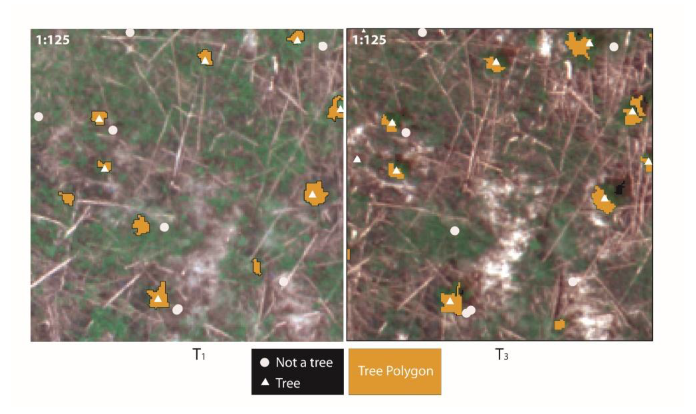
Figure 6.
Location of reference points for tree identification for T1 and T2 for plot A. Polygonal results of classification using Red-Edge images are also shown.
Figure 6.
Location of reference points for tree identification for T1 and T2 for plot A. Polygonal results of classification using Red-Edge images are also shown.

Figure 7.
Precipitation and Temperature recorded between 1 June 2017 and 31 August. Flights were performed on the 30th, 66th, and 80th dates, indicated by blue lines in the graphs above.
Figure 7.
Precipitation and Temperature recorded between 1 June 2017 and 31 August. Flights were performed on the 30th, 66th, and 80th dates, indicated by blue lines in the graphs above.

Figure 8.
Spectral Response Curve for jack pine saplings on Plot A at Time 1 and Time 3.


Table 1.
Specifications of MicaSense RedEdge 3 multispectral camera [31].
Table 1.
Specifications of MicaSense RedEdge 3 multispectral camera [31].
| Spectral Bands | Blue, Green, Red, Read Edge, NIR |
| Ground Sample Distance | 8.2 cm/pixel (per band) at 120 m Above Ground Level |
| Capture Speed | 1 capture per second (all bands) |
| Format | 12-bit Camera RAW |
| Focal Length/Field of View | 5.5 cm/47.2 degrees FOV |
| Image Resolution | 1280 × 960 pixels |
NIR—Near Infrared, FOV—Field of View.
Table 2.
Spectral specifications of MicaSense RedEdge 3 multispectral camera [31]. FWHM is short for full-width half maximum.
Table 2.
Spectral specifications of MicaSense RedEdge 3 multispectral camera [31]. FWHM is short for full-width half maximum.
| Band Number | Band Name | Center Wavelength (nm) | Bandwidth FWHM |
|---|---|---|---|
| 1 | Blue | 475 | 20 |
| 2 | Green | 560 | 20 |
| 3 | Red | 558 | 10 |
| 5 | Red Edge | 717 | 10 |
| 4 | Near IR | 840 | 40 |
Table 3.
Image acquisition campaign specifications.
| Plot | Flight | Images | Altitude (m) | Ground Resolution (m px−1) |
|---|---|---|---|---|
| A | T1 | 200 | 80 | 0.05505 |
| T2 | 200 | 0.05441 | ||
| T3 | 200 | 0.05513 | ||
| B | T3 | 190 | 80 | 0.05561 |
Table 4.
Accuracy results for Plot A and Plot B.
| Plot A | |||||
| Date | Bands | UA | PA | F-Score | CA |
| T1 | RE + NIR | 0.46 | 1.0 | 0.63 | 0.72 |
| NIR | 0.57 | 0.98 | 0.72 | 0.78 | |
| RE | 0.43 | 0.96 | 0.60 | 0.70 | |
| NIR − R | 0.60 | 0.94 | 0.73 | 0.78 | |
| T2 | RE + NIR | 0.50 | 1.0 | 0.66 | 0.75 |
| NIR | 0.50 | 1.0 | 0.66 | 0.75 | |
| RE | 0.54 | 1.0 | 0.82 | 0.69 | |
| NIR − R | 0.79 | 0.97 | 0.71 | 0.88 | |
| T3 | RE + NIR | 0.64 | 0.96 | 0.78 | 0.81 |
| NIR | 0.65 | 0.97 | 0.78 | 0.81 | |
| RE | 0.57 | 0.97 | 0.72 | 0.78 | |
| NIR − R | 0.79 | 0.97 | 0.87 | 0.88 | |
| Plot B | |||||
| Date | Bands | UA | PA | F-Score | CA |
| T3 | RE + NIR | 1.0 | 0.86 | 0.91 | 0.93 |
| NIR | 1.0 | 0.86 | 0.91 | 0.93 | |
| RE | 1.0 | 0.80 | 0.889 | 0.90 | |
| NIR − R | 1.0 | 0.95 | 0.79 | 0.98 | |
User accuracy (UA), producer accuracy (PA), count accuracy (CA), and F-score.
© 2018 by the authors. Licensee MDPI, Basel, Switzerland. This article is an open access article distributed under the terms and conditions of the Creative Commons Attribution (CC BY) license (http://creativecommons.org/licenses/by/4.0/).
Share and Cite
MDPI and ACS Style
White, R.A.; Bomber, M.; Hupy, J.P.; Shortridge, A. UAS-GEOBIA Approach to Sapling Identification in Jack Pine Barrens after Fire. Drones 2018, 2, 40. https://doi.org/10.3390/drones2040040
AMA Style
White RA, Bomber M, Hupy JP, Shortridge A. UAS-GEOBIA Approach to Sapling Identification in Jack Pine Barrens after Fire. Drones. 2018; 2(4):40. https://doi.org/10.3390/drones2040040
Chicago/Turabian StyleWhite, Raechel A., Michael Bomber, Joseph P. Hupy, and Ashton Shortridge. 2018. "UAS-GEOBIA Approach to Sapling Identification in Jack Pine Barrens after Fire" Drones 2, no. 4: 40. https://doi.org/10.3390/drones2040040