Sensitivity to Time Delays in VDM-Based Navigation

Abstract

A recently proposed navigation methodology for aerial platforms based on the vehicle dynamic model (VDM) has shown promising results in terms of navigation autonomy. Its practical realization requires that control inputs are related to the same absolute time frame as inertial measurement unit (IMU) data and all other observations when available (e.g., global navigation satellite system (GNSS) position, barometric altitude, etc.). This study analyzes the (non-) tolerances of possible delays in control-input command with respect to navigation performance on a fixed-wing unmanned aerial vehicle (UAV). Multiple simulations using two emulated trajectories based on real flights reveal the vital importance of correct time-tagging of servo data while that of motor data turned out to be tolerable to a considerably large extent.

1. Introduction

Inertial navigation system/global navigation satellite system (INS/GNSS) integration is currently the dominant navigation system used to provide satisfactory short-term and long-term accuracy for unmanned aerial robots. Problems emerge when outage occurs in GNSS signal reception, which can happen as a result of loss of line of sight with satellites, by suffering interference caused by nearby high-power transmitters or by the electronics on board the unmanned aerial vehicle (UAV) itself, or because of spoofing or intentional jamming. In this situation, the GNSS measurements become either untrustworthy or unavailable and the navigation solution is based only on INS in a dead-reckoning fashion. Its accuracy is directly determined by the quality of the inertial measurement units (IMUs), which has consequently become considerably lower. After only a few seconds of GNSS outage, the position uncertainty for small UAVs using low-cost IMUs goes beyond practical use, in the order of hundreds of meters or more [1].

Recently, there have been some research activities aimed at mitigating the problems of navigation during GNSS outages using vehicle dynamic models (VDM) [1,2,3,4,5]. In such navigation systems, the platform dependent dynamic model of the UAV is used in navigation as opposed to the platform-independent approach in INS-based navigation. The VDM is fed by the control input to the UAV and predicts the linear and rotational accelerations. The control input can be provided by different sources, such as the autopilot or the microcontrollers commanding the servos, depending on the architecture of the platform.

1.1. Motivation

It would be unrealistic to assume that the control input data are available for the navigation at the exact time they are emitted. In the navigation filter, these data need to be time-tagged to be attributed to a specific execution time, and there is always an inherent delay between subsystems that possess input and output signals. Such delays can be caused by the computational load, buffering mechanism, and signal propagation, to name only a few. Although the source(s) of such delays is not the topic of this study, it is nevertheless considered in the form of incorrect time-tagging of the control input data that is necessary to compute the VDM-based navigation solution. The impact of such time-tagging errors on navigation performance needs therefore to be investigated to confirm the feasibility of (or requirements on) the real-time implementation. To the best of the authors’ knowledge, such investigations have never been reported. The goal of this study is to assess quantitatively the influence of imperfect time-tagging on VDM-based navigation performance, and hence understand the limitations that those errors can impose on real implementation.

1.2. Proposed Approach

In order to assess the effects of imperfect time-tagging, the control input was artificially corrupted by different time delays along an emulated UAV-trajectory. Then, the position error of autonomous navigation was compared to the case with perfect (unperturbed) time-tagging. The VDM-based navigation system in this research follows from Reference [1]. The corruptions were made in a controlled way, and multiple simulations were performed with different noise realizations and then were averaged over all of the runs to gain statistical confidence on the conclusions.

Section 2 covers the background material necessary to describe the principle of the employed VDM-based navigation technique. Section 3 presents the methodology of this study by explaining each step of the simulation process. The findings and discussion are presented in Section 4, and Section 5 presents the conclusion.

2. VDM-Based Navigation

VDM (Vehicle Dynamic Model) is a mathematical model describing the motion dynamics for any particular UAV. At its core, VDM includes an aerodynamic model of forces and moments applied to the flying UAV. Based on that, VDM provides linear and rotational accelerations of the UAV, further used in the navigation. This applies the physical constraints on the motion of the UAV in navigation, and therefore improves the accuracy and reliability. VDM requires no extra sensors with respect to conventional navigation setup. It exploits the knowledge on platform dynamics and the UAV control inputs, which are normally available from the autopilot. Such a free source of information that is not benefited from in conventional navigation systems, is being utilized in VDM-based navigation to estimate trajectory parameters with a higher quality within the already available sensor setup. While the essentials of VDM-based navigation system is presented here shortly, more details can be found in [1].

2.1. Frames Definition

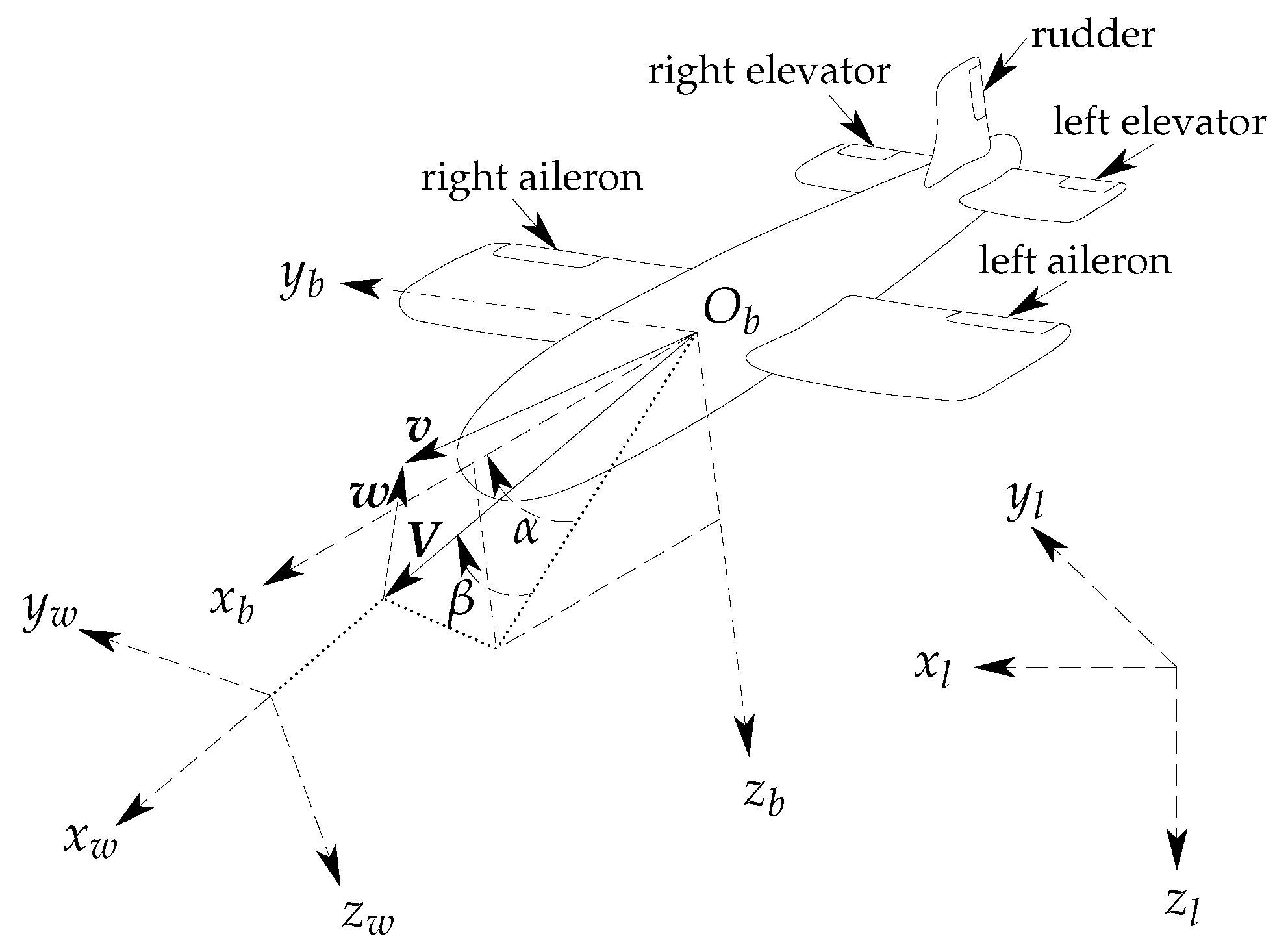
Five reference frames considered in this research are: “inertial”, “Earth”, “local level”, “body”, and “wind” frames. The inertial frame $(x_i,y_i,z_i)$ is an Earth centered inertial (ECI) frame, while the Earth frame $(x_e,y_e,z_e)$ is an Earth centered Earth fixed (ECEF) frame. The local-level frame is oriented in north, east, and down directions denoted by $(x_l,y_l,z_l)$ or $(x_N,x_E,x_D)$ with respect to the tangent plane on a reference ellipsoid [6]. Definitions of body frame $(x_b,y_b,z_b)$ and wind frame $(x_w,y_w,z_w)$ can be perceived from Figure 1.

The wind frame has its first axis in the direction of airspeed $\mathbf{V}$, and is defined by two angles with respect to body frame, angle of attack $\alpha$, and sideslip angle $\beta$. The velocity of airflow caused by the UAV’s inertial velocity $\mathbf{v}$ and wind velocity $\mathbf{w}$ is denoted by airspeed vector $\mathbf{V}$ as

$$\mathbf{V}=\mathbf{v}-\mathbf{w}.$$

(1)

The rotation matrix ${\mathbf{C}}_b^w$ from body frame to wind frame is defined as a function of angle of attack $\alpha$ and sideslip angle $\beta$ as

$${\mathbf{C}}_b^w={\mathbf{R}}_3\left(\beta \right){\mathbf{R}}_2\left(\alpha \right),$$

(2)

where ${\mathbf{R}}_i$ denotes the elementary rotation matrix around the i-th axis.

2.2. Vehicle Dynamic Model (VDM)

Contrary to References [2,3,4,5], Earth rotation and curvature are considered in this paper as in Reference [1]. Quaternions are used for attitude representation instead of Euler angles to avoid singularities. The VDM kinematics is presented in state space form, the model of which is

$${\mathbf{X}}_n={\left[{{\mathbf{r}}_e^l}^T,{{\mathbf{v}}_e^l}^T,{{\mathbf{q}}_b^l}^T,{{\mathit{\omega }}_{ib}^b}^T\right]}^T,$$

(3)

where ${{\mathbf{r}}_e^l}^T=[\varphi ,\lambda ,h]$ is the platform position in geographical ellipsoidal coordinates, ${{\mathbf{v}}_e^l}^T=[V_N,V_E,V_D]$ is the velocity, ${{\mathbf{q}}_b^l}^T=[q_0,\dots ,q_4]$ is the attitude, and ${{\mathit{\omega }}_{ib}^b}^T=[{\omega }_1,{\omega }_2,{\omega }_3]$ the angular rate in vector or skew-symmetric ${\mathbf{\Omega }}_{ib}^b$ form.

The dynamic model is expressed as [1,7]

$$\begin{array}{c}{\dot{\mathbf{r}}}_e^l={\mathbf{D}}^{-1}{\mathbf{v}}_e^l\hfill \end{array}$$

(4)

$$\begin{array}{c}{\dot{\mathbf{v}}}_e^l={\mathbf{C}}_b^l{\mathbf{f}}^b+{\mathbf{g}}^l-({\mathbf{\Omega }}_{el}^l+2{\mathbf{\Omega }}_{ie}^l){\mathbf{v}}_e^l\hfill \end{array}$$

(5)

$$\begin{array}{c}{\dot{\mathbf{q}}}_b^l=\frac{1}{2}{\mathbf{q}}_b^l\otimes {\left[{\mathit{\omega }}_{lb}^b\right]}_q\hfill \end{array}$$

(6)

$$\begin{array}{c}{\dot{\mathit{\omega }}}_{ib}^b={\left({\mathbf{I}}^b\right)}^{-1}\left[{\mathbf{M}}^b-{\mathbf{\Omega }}_{ib}^b\left({\mathbf{I}}^b{\mathit{\omega }}_{ib}^b\right)\right],\hfill \end{array}$$

(7)

where the skew-symmetric matrix representation of any ${\mathit{\omega }}_{pq}^r={\left[\begin{array}{ccc}{\omega }_1& {\omega }_2& {\omega }_3\end{array}\right]}^T$ vector is represented by ${\mathbf{\Omega }}_{pq}^r$ as

$${\mathbf{\Omega }}_{pq}^r=\left[\begin{array}{ccc}0& -{\omega }_3& {\omega }_2\\ {\omega }_3& 0& -{\omega }_1\\ -{\omega }_2& {\omega }_1& 0\end{array}\right].$$

(8)

The matrix ${\mathbf{D}}^{-1}$ in Equation (4) is defined as

$${\mathbf{D}}^{-1}=\left[\begin{array}{ccc}\frac{1}{R_M+h}& 0& 0\\ 0& \frac{1}{(R_P+h)cos\varphi }& 0\\ 0& 0& -1\end{array}\right],$$

(9)

where $R_P$ and $R_M$ represent the prime vertical radius of curvature and meridian radius of curvature, respectively. The rotation matrix ${\mathbf{C}}_b^l$ in Equation (5) is a function of the quaternion ${\mathbf{q}}_b^l$ as

$$\begin{array}{c}{\mathbf{C}}_b^l=f\left({\mathbf{q}}_b^l\right)=\hfill \\ \left[\begin{array}{ccc}{q}_0^2+q_1^2-q_2^2-q_3^2& 2(q_1{q}_2-q_0{q}_3)& 2(q_1{q}_3+q_0{q}_2)\\ 2(q_1{q}_2+q_0{q}_3)& q_0^2-q_1^2+q_2^2-q_3^2& 2(q_2{q}_3-q_0{q}_1)\\ 2(q_1{q}_3-q_0{q}_2)& 2(q_2{q}_3+q_0{q}_1)& q_0^2-q_1^2-q_2^2+q_3^2\end{array}\right],\hfill \end{array}$$

(10)

and ${\mathbf{g}}^l$ represents the gravity vector. The ${\mathit{\omega }}_{lb}^b$ vector in Equation (6) is calculated as

$${\mathit{\omega }}_{lb}^b={\mathit{\omega }}_{ib}^b-{\left(C_b^l\right)}^T\left({\mathit{\omega }}_{ie}^l+{\mathit{\omega }}_{el}^l\right),$$

(11)

where ${\mathit{\omega }}_{ie}^l$ and ${\mathit{\omega }}_{el}^l$ are defined as follows:

$$\begin{array}{c}{\mathit{\omega }}_{ie}^l={\left[\begin{array}{ccc}{\omega }_{ie}cos\varphi & 0& -{\omega }_{ie}sin\varphi \end{array}\right]}^T\hfill \end{array}$$

(12)

$$\begin{array}{c}{\mathit{\omega }}_{el}^l={\left[\begin{array}{ccc}\dot{\lambda }cos\varphi & -\dot{\varphi }& \dot{\lambda }sin\varphi \end{array}\right]}^T.\hfill \end{array}$$

(13)

The matrix ${\mathbf{I}}^b$ in Equation (7) denotes the moments of the inertia matrix.

The presented model is the general dynamic model for any rigid body affected by external specific force $\mathbf{f}$, external moment $\mathbf{M}$, and Earth gravity $\mathbf{g}$. For a specific type of UAV, fixed-wing for example, an aerodynamic model defines specific force vector $\mathbf{f}$ and the moments vector $\mathbf{M}$ as follows, with m denoting the mass of the UAV:

$$\begin{array}{c}{\mathbf{f}}^b=\frac{1}{m}(\left[\begin{array}{c}{F}_T\\ 0\\ 0\end{array}\right]+C_w^b\left[\begin{array}{c}{F}_x^w\\ F_y^w\\ F_z^w\end{array}\right])\hfill \end{array}$$

(14)

$$\begin{array}{c}{\mathbf{M}}^b=\left[\begin{array}{c}{M}_x^b\\ M_y^b\\ M_z^b.\end{array}\right]\hfill \end{array}$$

(15)

Thrust, drag, lateral, and lift forces ($F_T$, $F_x^w$, $F_y^w$, and $F_z^w$, respectively) are the four components of aerodynamic forces. Roll, pitch, and yaw moments ($M_x^b$, $M_y^b$, and $M_z^b$, respectively) are the three components of aerodynamic moments. While thrust force (along $x_b$-axis) and all moment components are expressed in body frame, lift, lateral, and drag forces are expressed in wind frame:

$$\begin{array}{c}{F}_T=\rho n^2{D}^4\left(C_{F_{T}1}+C_{F_{T}2}J+C_{F_{T}3}{J}^2\right)\hfill \end{array}$$

(16)

$$\begin{array}{c}{F}_x^w=\overline{q}S\left(C_{F_{x}1}+C_{F_x\alpha }\alpha +C_{F_x\alpha 2}{\alpha }^2+C_{F_x\beta 2}{\beta }^2\right)\hfill \end{array}$$

(17)

$$\begin{array}{c}{F}_y^w=\overline{q}S\left(C_{F_{y}1}\beta \right)\hfill \end{array}$$

(18)

$$\begin{array}{c}{F}_z^w=\overline{q}S\left(C_{F_{z}1}+C_{F_z\alpha }\alpha \right)\hfill \end{array}$$

(19)

$$\begin{array}{c}{M}_x^b=\overline{q}Sb\left(C_{M_{x}a}{\delta }_a+C_{M_x\beta }\beta +C_{M_x{\tilde{\omega }}_x}{\tilde{\omega }}_x+C_{M_x{\tilde{\omega }}_z}{\tilde{\omega }}_z\right)\hfill \end{array}$$

(20)

$$\begin{array}{c}{M}_y^b=\overline{q}S\overline{c}\left(C_{M_{y}1}+C_{M_{y}e}{\delta }_e+C_{M_y{\tilde{\omega }}_y}{\tilde{\omega }}_y+C_{M_y\alpha }\alpha \right)\hfill \end{array}$$

(21)

$$\begin{array}{c}{M}_z^b=\overline{q}Sb\left(C_{M_z{\delta }_r}{\delta }_r+C_{M_z{\tilde{\omega }}_z}{\tilde{\omega }}_z+C_{M_z\beta }\beta \right)\hfill \end{array}$$

(22)

where b, S, $\overline{c}$, and D are geometric measures of the UAV representing wing span, wing surface, mean aerodynamic chord, and propeller diameter, respectively. Air density is denoted by $\rho$, while $\overline{q}$ is dynamic pressure defined as $\rho V^2/2$, and J is defined as $V/\left(D\pi n\right)$ with n denoting propeller speed. Dimensionless angular velocities are defined as ${\tilde{\omega }}_x=b{\omega }_x/\left(2V\right)$, ${\tilde{\omega }}_y=\overline{c}{\omega }_y/\left(2V\right)$, and ${\tilde{\omega }}_z=b{\omega }_z/\left(2V\right)$. The aerodynamic coefficients for the particular UAV at hand are represented by $C_{\dots }$’s, and deflections of aileron, elevator, and rudder are denoted by ${\delta }_a$, ${\delta }_e$, and ${\delta }_r$, respectively.

The required inputs for the aerodynamic model are dynamic (navigation) states, wind velocity, control inputs, and physical parameters of the UAV. As depicted schematically in Figure 1, the UAV type considered in this paper has a single propeller, as well as aileron, elevator, and rudder control surfaces. The aerodynamic model for this UAV type is borrowed from Reference [8], while adapting the physical parameters.

2.3. Navigation System

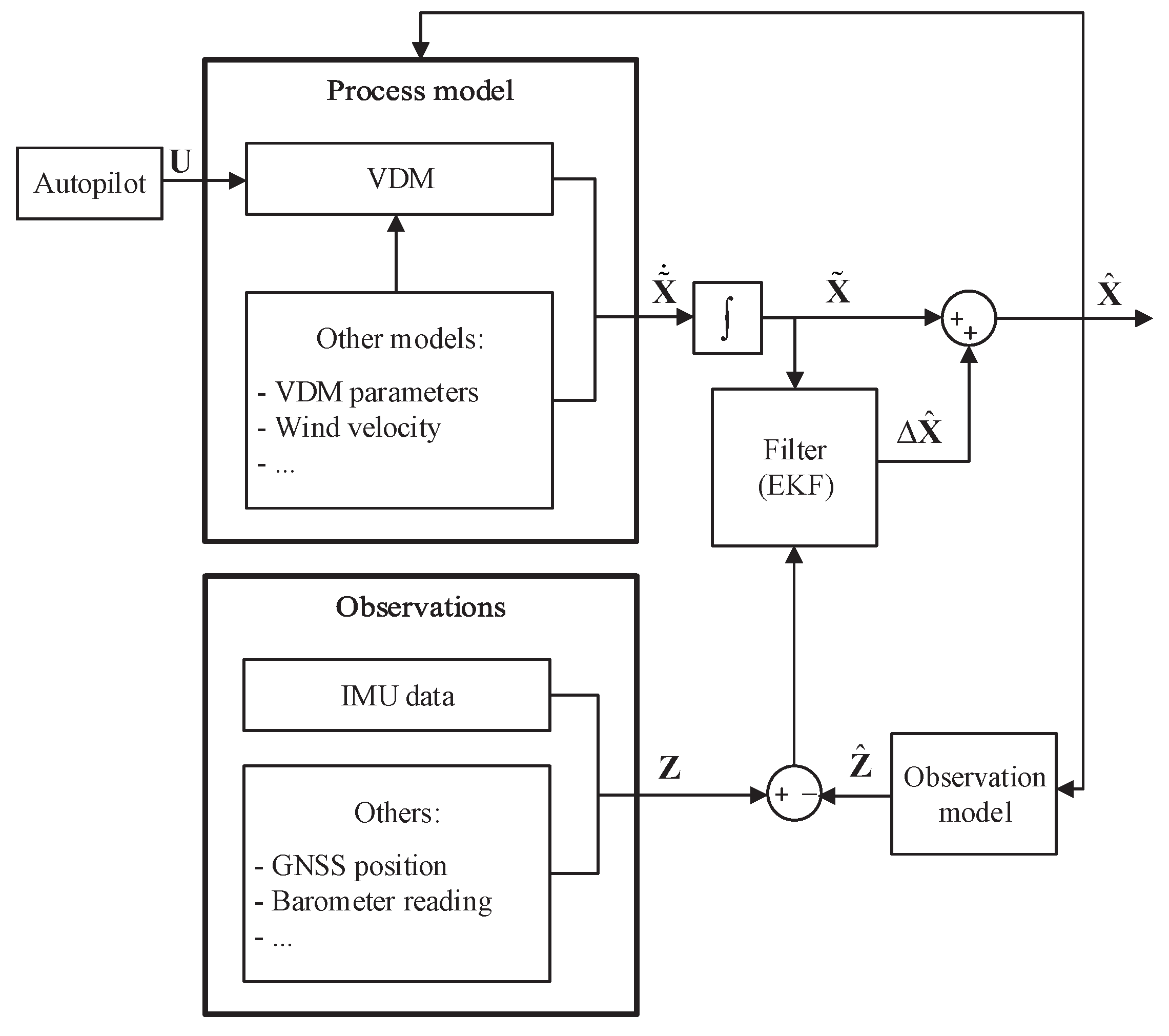
In the proposed navigation system, the VDM serves as the main process model within the filter. A standard extended Kalman filter (EKF) [9] is chosen in this paper to estimate corrections to the states ($\Delta \mathbf{X}$) and the associated covariance matrix (P). More detailed description of process models, observation models, and their linearization for proposed VDM-based navigation can be found in Reference [1].

As depicted in Figure 2, the VDM provides the navigation solution (${\mathbf{X}}_n$), which gets updated as a part of the augmented state vector $\mathbf{X}$ (introduced in Equation (24) based on the available observations. Since IMU data are treated as observations, in case of an IMU failure, the navigation system stops using IMU data and provides the navigation solution using only the VDM and other available observations. Observations from other sensors such as the airspeed sensor, optic flow sensor, and magnetometer can also be integrated within the navigation system.

The VDM is fed with the control input ($\mathbf{U}$) to the UAV as commanded by the autopilot and therefore is always available. Wind velocity (${\mathbf{X}}_w$) is also required, which can be estimated within the navigation system, even in the absence of airspeed sensors, which is the case here [10]. The required VDM parameters (${\mathbf{X}}_p$) can be pre-calibrated and used as fixed values in the navigation system or estimated in-flight/refined from them. The latter option is implemented to increase flexibility and accuracy of the proposed approach while minimizing design effort.

The augmented state vector $\mathbf{X}$ includes navigation states ${\mathbf{X}}_n$, VDM parameters ${\mathbf{X}}_p$, and wind velocity components ${\mathbf{X}}_w$.

$$\mathbf{X}={[{\mathbf{X}}_n^T,{\mathbf{X}}_p^T,{\mathbf{X}}_w^T]}^T$$

(23)

Mass $\left(m\right)$ and moments of inertia ${\mathbf{I}}^b$ are excluded from ${\mathbf{X}}_p$ since they appear as scaling factors in the model, which means they are completely correlated with the already included aerodynamic coefficients [1]. Geometric measures are also excluded, because they can be determined a priori with much lower uncertainty compared to aerodynamic coefficients. If IMU data are available, their error, such as their biases, can also be included within the augmented states vector [1].

3. Methodology

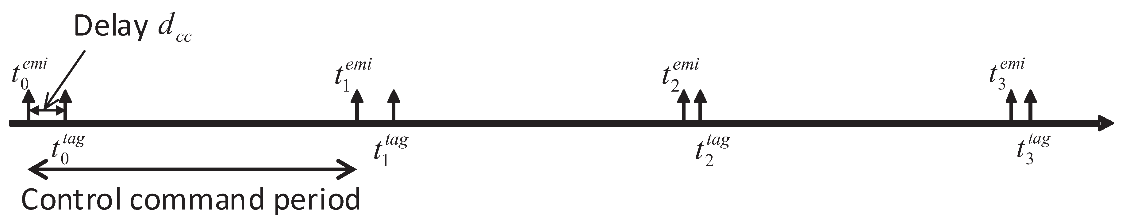
The control input (U), as depicted in Figure 2, is fed to the VDM. In an ideal real-time implementation, the control input data should be read directly from the microcontroller that commands those inputs. For the platform used in this research, the actuators include two servos for the ailerons, one servo for the rudder, one servo for the elevator, and one motor to spin the propeller. The control input (U) is the $5\times 1$ vector of the commands setting the defection of aileron (the two combined in a differential manner), elevator, and rudder, as well as the rotational speed of the propeller. In most systems, the control commands can only be accessed from the on-board computer that hosts the autopilot. The latter time-tags the data with its own system time. The data time-tagging operation requires its own processing time and depending on the system computational load, some delays can be expected between the time a control command is emitted $t_0^{emi}$ and the time when it is time-tagged $t_0^{tag}$. This is illustrated in Figure 3.

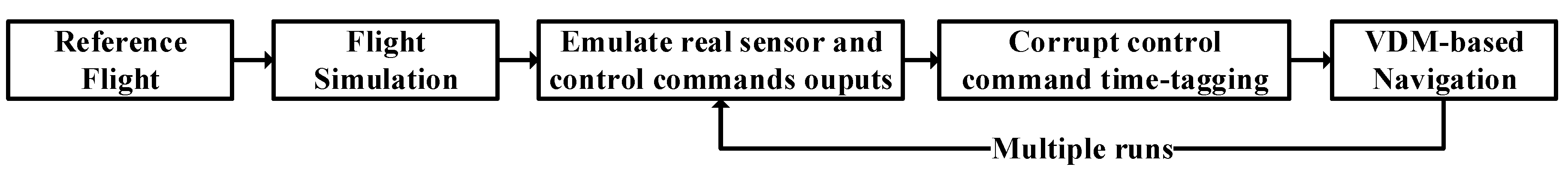
In order to assess the influence of imperfections in data time-tagging on the performance of VDM-based navigation, a simulation scenario was setup. The steps of this simulation are depicted in Figure 4 and are detailed as follows:

3.1. Reference and Flight Simulation

The UAV used for this study is a custom made airplane equipped with the open-source autopilot Pixhawk [11]. Its operational weight is around 2.5 kg, depending on the payload, and nominal airspeed is around 15 m/s. The geometrical details of the platform are given in Reference [1]. The navigation sensors include a MEMS IMU called Navchip [12] on a custom board with a barometer. A geodetic grade GNSS receiver is on board, capable of working in real time kinematic (RTK) mode, although only the stand-alone solution is used in navigation. The sampling frequencies are 100 Hz for the IMU, 10 Hz for the barometer, and 1 Hz for the stand-alone GNSS position and velocity data.

To obtain a realistic stochastic model for IMU errors, an in-house identification was performed, using the novel approach of generalized method of wavelet moments (GMWM) [13]. A summary of the IMU error parameters from the GMWM analysis is provided in

Table 1. MEMS inertial measurement unit (IMU) error statistics.

Sensor	Error Type	Parameter	Value	Unit
Accelero-meters	Bias	$\sigma$	8	mg
	White Noise	$\sigma$	67	$\mathsf{\mu }$g/$\sqrt{\mathrm{Hz}}$
	1st order Gauss–Markov	$\sigma$	0.15	mg
		T	200	s
Gyro-scopes	Bias	$\sigma$	720	${}^{\circ }$/h
	White Noise	$\sigma$	0.005	${}^{\circ }/\mathrm{s}/\sqrt{\mathrm{Hz}}$
	1st order Gauss–Markov	$\sigma$	31	${}^{\circ }$/h
		T	200	s

.

GNSS position and velocity errors are considered as Gaussian white noise with $\sigma$ = 1 m and $\sigma$ = 0.03 m/s, respectively, for each horizontal channel and $\sigma$ = 2 m and $\sigma$ = 0.04 m/s for the vertical channel. The error in barometric altitude data is also considered as a Gaussian white noise with $\sigma$ = 0.5 m. This noise level is determined based on experimental data when barometer output was compared to post processed cm-level GNSS position as the reference.

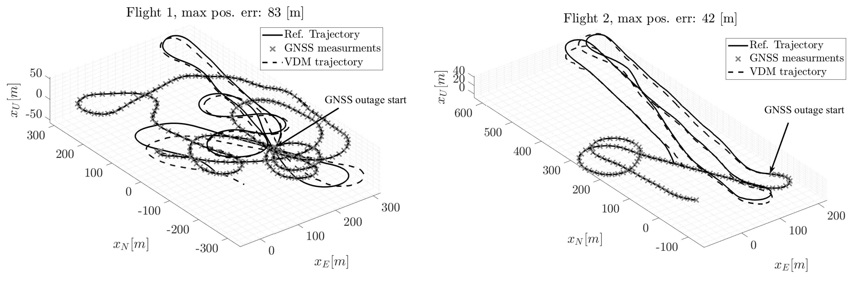
Two flights were considered, reference trajectories of which are shown in Figure 5. The first flight, denoted as Flight 1 hereinafter, lasted 425 s; while the second flight, hereinafter referred to as Flight 2, lasted 272 s. Both flights were performed using the custom fixed-wing UAV introduced in Section 3.1. PPK (PPK = Post-Processed Kinematic = carrier-phase differential GNSS) GNSS solution with cm-level accuracy was used to generate way points to emulate the flights in the simulations.

Once the way points were generated from real flight data, the flights were simulated using the model described in Section 2.2, and corresponding error-free sensor data (IMU, GNSS, and barometer) were emulated, as were the control commands. Sensor errors were added to the emulated data afterwards according to the description in Table 1. As this study aims to assess the effects of time-tagging errors in the control input only, emulated sensor readings were introduced to avoid mixing the effects with additional errors.

3.2. Time-Tagging Errors

At this point, the time-tagging of control input data was corrupted by adding some stochastic delay to simulate a realistic case. The nature of such delay in real cases depends on the internal properties of the system and is not known exactly. In this study, time delays of control command $d_{cc}$ were modeled as the sum of a constant bias b and a positive random delay w as

$$d_{cc}\left(n\right)=b+\left|w\left(n\right)\right|,$$

(24)

where $w\sim \mathcal{N}(0,{\sigma }^2)$. The impact of time-tagging on errors in VDM-based navigation was studied for different values of b and $\sigma$.

The control commands were separated into two groups: those related to motor propeller speed (rpm) and to the servos (for aileron, elevator, and rudder). The servo and motor rpm commands were assumed to be accessible at 10 Hz, which is the case on the employed UAV. The ideal time-tagging of the data was corrupted by delay $d_{cc}$ for each data set separately. The meaning of the emitted and tagged times is illustrated in Figure 3.

The navigation and filtering in the simulation was set to 100 Hz, but it also ran every time a new control input (with corrupted time-tagging) was available in the process. This guarantees that no additional delay was introduced by the processing scheme as a result of buffering.

3.3. VDM-Based Navigation

When the motor and servo time-tagging was corrupted for a particular fixed delay and absolute noise error level, VDM-based navigation was performed on the data. For both flights, 3 min long GNSS outage was considered before the trajectory ended. Maximum position errors were saved for each run with the same added timing error characteristics. For this research, there were 15 runs for every combination of fixed and random delays, each with a different noise realization.

4. Results and Discussion

This section analyzes the influence of time-tagging errors on VDM-based navigation for the two trajectories presented in Section 3.1.

First, VDM-based navigation with 3 min of GNSS outage without any time-tagging error was performed as the reference and presented as the solid line in Figure 5. Then, cases with different levels of delays were simulated separately for motor and servo commands. The corresponding maximum error in position at the end of 3 minute long autonomous navigation was 83 m for Flight 1 and 42 m for Flight 2. It can be observed that the autonomous VDM-based navigation solution drifted somewhat in both flights, though the resulting trajectory still qualitatively followed the reference one. INS-based navigation was not able to produce a result with nearly as competitive a result for the same level of noise in the inertial data.

4.1. Motor Data Time-Tagging Errors

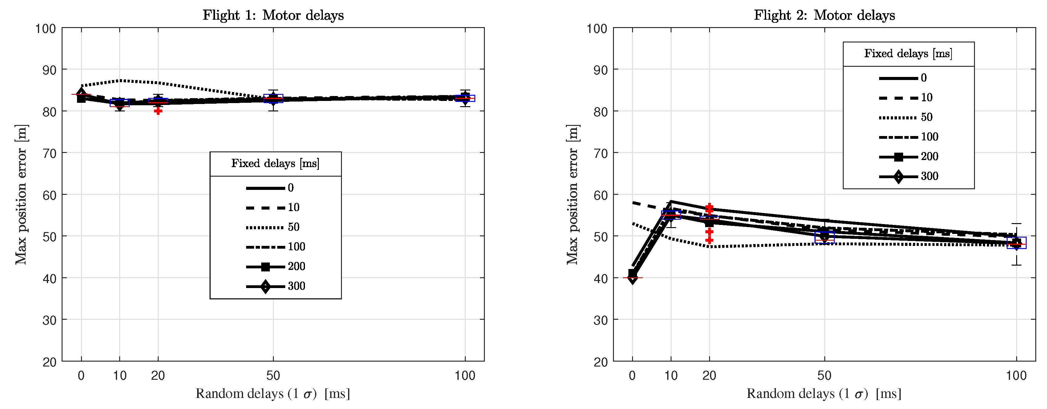
The investigated motor data time-tagging errors range from 0 to 300 ms of fixed delay plus a random noise delay of standard deviation from 0 to 100 ms. The considered values are presented in

Table 2. Fixed and random delays for motor data.

Fixed Delays [ms]	Random Delays [ms]
0	0
10	10
50	20
100	50
200	100
300	∅

.

Figure 6 depicts the average of the maximum position error for all runs. The max. error in position for all runs for the larger fixed delay considered (300 ms) are presented as a box-plot. In each box, the central mark indicates the median of all runs, and the bottom and top edges of the box indicate the 25th and 75th percentiles, respectively. The whiskers extend to the most extreme data points not considered outliers. The outliers are plotted individually using red ‘+’ symbol. The motor time-tagging errors seem not to introduce a noticeable deterioration of VDM-based navigation performance compared to the case with perfect time-tagging. A possible reason is the slow dynamic response of the UAV to the propeller speed, which creates the relatively small time-tagging errors (with respect to associated dynamic modes of the UAV) causing very little impact on navigation. Indeed, the absence of wind in the simulation and the nominal and almost constant velocity of the platform during both trajectories imply a very low dynamic in the change of propeller speed, simplifying the model. Larger errors in position are expected if those two conditions are different, i.e., wind is present or added in the simulation and the platform changes its velocity during the flight.

4.2. Servos Data Time-Tagging Errors

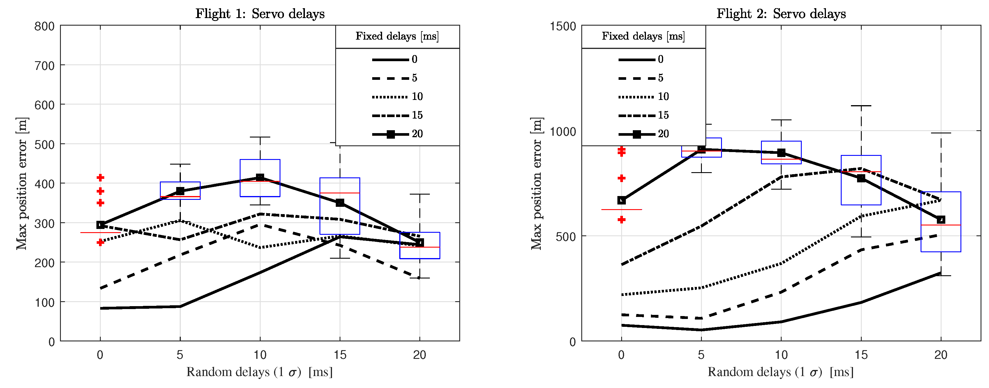
Considering the high sensitivity of UAV dynamic response to servo data time-tagging errors, the chosen fixed delay and random noise standard deviation were limited within a range from 0 to 20 ms as shown in

Table 3. Fixed and random delays for servos data.

Fixed Delays [ms]	Random Delays [ms]
0	0
5	5
10	10
15	15
20	20

. The effect of those errors on max. error in position is plotted in Figure 7.

The error growth in position is noticeable when time-tagging error of servo data increases. It is interesting to notice that the evolution of the errors with random delay follows a different trend per fixed delay. This may be due to relatively low number of runs per each (of many) combination. Despite larger delays also being tested, these are not presented as to stay with the main objective: identifying the main tendency of position error growth. A fixed delay of only 10 ms increases the max. error in position more than three times, even with no random delay. This reveals the importance of proper time-tagging of control input data for VDM-based navigation.

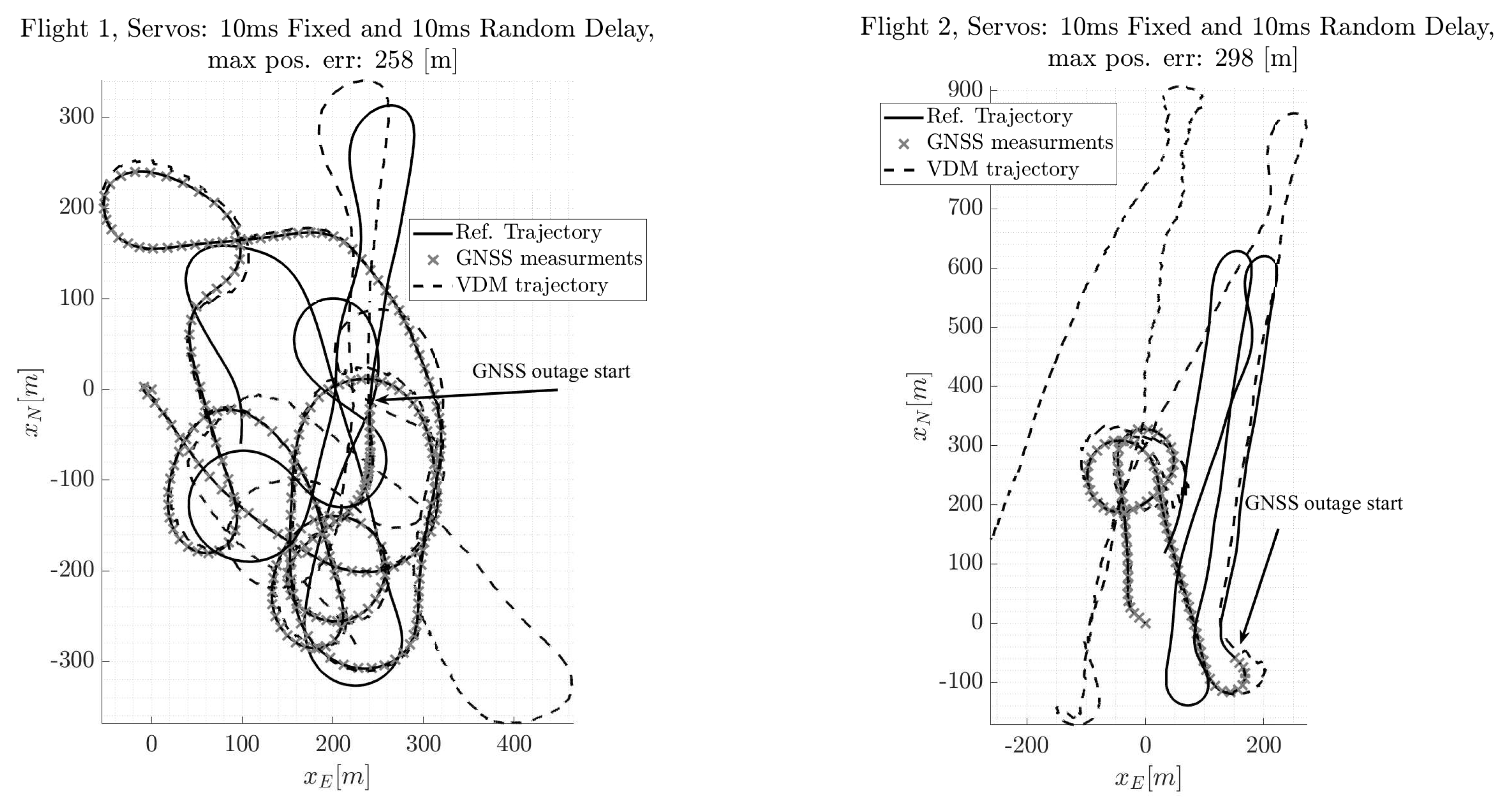
Figure 8 shows the VDM-based navigation solution both with an introduced fixed and random (standard deviation) delay of 10 ms in the servo data for a particular run. The maximum position error during a GNSS outage for both flights is around 300 m, i.e., about three times larger than the nominal scenario, although the trajectory dependency of dead reckoning methods makes the direct comparison between trajectories less relevant. Note that the magnitude of vertical errors are limited by the barometer measurements. In addition, as explained in Section 2.3, there is an in-flight refinement of the VDM parameters when GNSS data are available. Flight 1 lasted 152 s longer than Flight 2 and experienced more dynamic maneuvers, therefore it is reasonable to expect a finer estimation of the VDM parameters resulting in a slightly better performance in autonomous navigation.

Simulations were also performed combining time-tagging errors for both motor and servo data. However, when compared with servo errors only, the difference with the addition of time-tagging errors for the motor input was almost negligible. Therefore, these results are not presented.

5. Conclusions and Perspectives

This investigation assessed the influence of time-tagging errors in control input on VDM-based navigation of a fixed-wing UAV.

Two real flights were used to emulate sensor and control input data. The time-tagging of the latter was then corrupted by a combination of fixed (bias) and random (noise) delays and the effects analyzed via averaged simulations. Thereafter, the performance of VDM-based navigation was represented by the maximum position error after 3 min of GNSS outage. For both trajectories, time-tagging errors in the motor data were observed to have negligible influence on the maximum position error for all fixed and random delays considered. On the other hand, the impact of time-tagging errors in the servo data was indisputably higher. A rapid growth in the position error was observed even for delays as small as ten of milliseconds.

The results for both flights reveal a correlation with the trajectory characteristics, which is generally relevant for both kinematic as well as dynamic-based modeling. Therefore, maximum position error is not necessarily the most pertinent criterion to assess the performance of the VDM-based navigation solution. Nevertheless, it provides a bulk estimation for the engineering requirements on time-tagging realization in fixed-wing UAVs.

Further experiments could be run on rotary-wing UAVs. The influence of the motor time-tagging error for rotary-wings is expected to be more pronounced, as the speeds of propellers are the only control input for such platforms and directly affect both translation and rotational dynamics.

References

- Khaghani, M.; Skaloud, J. Assessment of VDM-based Autonomous Navigation of a UAV under Operational Conditions. Robot. Auton. Syst. 2018, 106, 152–164. [Google Scholar]
- Koifman, M.; Bar-Itzhack, I.Y. Inertial navigation system aided by aircraft dynamics. IEEE Trans. Control Syst. Technol. 1999, 7, 487–493. [Google Scholar] [CrossRef]
- Cork, L.R. Aircraft Dynamic Navigation for Unmanned Aerial Vehicles. Ph.D. Thesis, Queensland University of Technology, Brisbane, Australia, 2014. [Google Scholar]
- Bryson, M.; Sukkarieh, S. UAV Localization Using Inertial Sensors and Satellite Positioning Systems. In Handbook of Unmanned Aerial Vehicles; Springer: Dordrecht, The Netherlands, 2015; pp. 433–460. [Google Scholar]
- Crocoll, P.; Seibold, J.; Scholz, G.; Trommer, G.F. Model-Aided Navigation for a Quadrotor Helicopter: A Novel Navigation System and First Experimental Results. Navigation 2014, 61, 253–271. [Google Scholar] [CrossRef]
- NIMA WGS84 Update Committee. Department of Defense. World Geodetic System 1984, Its Definition and Relationships with Local Geodetic Systems, 3rd ed.; Technical Report; National Imagery and Mapping Agency: Springfield, VA, USA, 2000.
- Stebler, Y. Modeling and Processing Approaches for Integrated Inertial Navigation. Ph.D. Thesis, EPFL, Lausanne, Switzerland, 2013. [Google Scholar]
- Ducard, G. Fault-Tolerant Flight Control and Guidance Systems: Practical Methods for Small Unmanned Aerial Vehicles; Springer: London, UK, 2009. [Google Scholar]
- Gelb, A. (Ed.) Applied Optimal Estimation; The MIT Press: Cambridge, MA, USA, 1988. [Google Scholar]
- Khaghani, M.; Skaloud, J. Evaluation of Wind Effects on UAV Autonomous Navigation Based on Vehicle Dynamic Model. In Proceedings of the 29th International Technical Meeting of The Satellite Division of the Institute of Navigation (ION GNSS+ 2016), Portland, OR, USA, 12–16 September 2016; pp. 1432–1440. [Google Scholar]
- Meier, L.; Tanskanen, P.; Heng, L.; Lee, G.H.; Fraundorfer, F.; Pollefeys, M. PIXHAWK: A Micro Aerial Vehicle Design for Autonomous Flight using Onboard Computer Vision. Auton. Robots 2012, 33, 21–39. [Google Scholar] [CrossRef]
- Intersense. Navchip. Available online: http://www.intersense.com/pages/16/246 (accessed on 10 December 2015).
- Guerrier, S.; Skaloud, J.; Stebler, Y.; Victoria-Feser, M.P. Wavelet-Variance-based Estimation for Composite Stochastic Processes. J. Am. Stat. Assoc. 2013, 108, 1021–1030. [Google Scholar] [PubMed]
Figure 1.
Local level, body, and wind frames with airspeed , wind velocity , and unmanned aerial vehicle (UAV) velocity [1].
Figure 2.
Vehicle dynamic model (VDM)-based navigation filter architecture ().
Figure 3.
Time-tagging of the emitted control commands with delays.
Figure 4.
Flowchart of simulations to assess effect of time-tagging errors.
Figure 5.
Reference trajectory and navigation solution with perfect time-tagging.
Figure 6.
Maximum position error averaged over all runs with motor time-tagging errors.
Figure 7.
Maximum position error averaged over all runs with servo time-tagging errors.
Figure 8.
Reference trajectory and navigation solution with sample servos time-tagging error.