Towards a Model Based Sensor Measurement Variance Input for Extended Kalman Filter State Estimation
by
 , , and
Harry A. G. Pointon
1,* ,
,
Benjamin J. McLoughlin
1,
Christian Matthews
2 and
Frederic A. Bezombes
1,* 1
Engineering and Technology Research Institute, Liverpool John Moores University, 3 Byrom St, Liverpool L3 3AF, UK
2
Department of Maritime and Mechanical Engineering, Liverpool John Moores University, 3 Byrom St, Liverpool L3 3AF, UK
*
Authors to whom correspondence should be addressed.
Drones 2019, 3(1), 19; https://doi.org/10.3390/drones3010019
Submission received: 8 January 2019
/
Revised: 7 February 2019
/
Accepted: 12 February 2019
/
Published: 14 February 2019
(This article belongs to the Special Issue Drones Navigation and Orientation)
Abstract
:In this paper, we present an alternate method for the generation and implementation of the sensor measurement variance used in an Extended Kalman Filter (EKF). Furthermore, it demonstrates the limitations of a conventional EKF implementation and postulates an alternate form for representing the sensor measurement variance by extending and improving the characterisation methodology presented in the previous work. As presented in earlier work, the use of surveying grade optical measurement instruments allows for a more effective characterisation of Ultra-Wide Band (UWB) localisation sensors; however, in cluttered environments, the sensor measurement variance will change, making this method not robust. To compensate for the noisier readings, an EKF using a model based sensor measurement variance was developed. This approach allows for a more accurate representation of the sensor measurement variance and leads to a more robust state estimation system. Simulations were run using synthetic data in order to test the effectiveness of the EKF against the originally developed EKF; next, the new EKF was compared to the original EKF using real world data. The new EKF was shown to function much more stably and consistently in less ideal environments for UWB deployment than the previous version.
1. Introduction
Positional assurance is an imperative and heavily researched area within unmanned robotic systems and technology [1]. The ability to precisely estimate a robot position, or for the robot to be capable of localising itself within the environment, is a vital topic to consider prior to the integration of such autonomous systems into modern day operations [2]. The ability to assess the effectiveness of such a system is a direct requirement for Beyond Visual Line Of Sight (BVLOS) operation [3]. BVLOS is usually considered at ranges greater at 500 m. However, BVLOS operation may also be considered within short range, enclosed cluttered environments involving buildings or obstructions and/or where transitions between indoor and outdoor environments may occur [4]. A traditional and well-documented technique commonly deployed for this purpose is Global Navigation Satellite Systems (GNSS) [5,6,7]. However, GNSS experiences shortcomings in certain environments such as mountainous terrains and urban areas, where an agglomeration of tall structures can cause loss of signal or multi-path effects. Many other techniques have been implemented with the aim to estimate the state of a mobile robot, notable implementations include the deployment of vision-based techniques such as monocular and stereo visual odometry systems, where the former is usually accompanied with an additional sensor to scale the output [8]. Other implementations also include odometry estimation through acoustic, dead reckoning and laser odometry, where scan matching algorithms are used to estimate the motion of the robot through 2D feature tracking [2]. Different categories of sensors all function using differing variable measurements and measurement methods, therefore the performance of each category of sensor is also dissimilar depending upon external factors, such as environments and operating conditions [2].
State estimation systems such as the Kalman Filter (KF) and its many variants represent a common implementation of recursive state estimation systems [2,9]. These systems estimate an updated state based upon a kinematic model of the system, measurement inputs and measurement variance. The main aspect to consider within sensor performance in robotics is the issue of variance. Variance is a critical element of robotics and is generally affected by factors such as unpredictable environments, accumulated variance and inaccurate mathematical system modelling [9]. Therefore, it is common practice to integrate multiple sources of information in an attempt to compliment the errors and uncertainties of each source of information [2,10]. This area of robotics is known as sensor fusion, where data acquired from multiple sensors is fused within state estimation algorithms such as the Kalman Filter and its many variants for both linear and nonlinear system models. The Kalman Filter takes into account the variance metric in the form of a covariance matrix for all sources of information that is channelled into the filter. For this work, the variance metric for an Ultra-Wide-Band (UWB) localisation system is assessed. A challenge in the formulation of state estimation systems is the calculation or experimental determination of sensor variance.
As demonstrated in previous work, the use of a Robotic Total Station allows for a significantly more accurate means of empirical modelling of the sensor measurement variance of localisation systems [11]. From this, an effective EKF system was designed and shown to function well in its intended environment in comparison to the raw UWB positioning algorithm [11]. However, under circumstances where the UWB antenna placement is non-ideal, the variance of the measurements will suffer, therefore decreasing the effectiveness of the conventional EKF. Modelling the variance of a sensor as a transient variable rather than constant enables a more representative variance to be obtained, by taking into account the changing nature of the sensor measurement variance. This variable may be a function of environmental factors, a component of the agents state or range to the UWB anchor node. In conventional terms, the sensor measurement variance is defined as a constant either as a whole or for discrete dimensions [9]. This may be termed a generalised variance as it is invariant to changes in the environment and represents the general variance of the sensor. The work conducted in this paper presents the development of a model-based variance that is represented as a function of UWB rover-anchor node range. As the rover position varies, the variance of the UWB sensor network will shift in response to a change in UWB range [12]. This methodology is empirically verified against the previously formulated EKF in a simulated scenario, and a more challenging environment than previously used.
1.1. Ultra Wide-Band Positioning
The method of operation of the UWB system has been described variously in previous works [11,13,14]. For the purposes of the study presented in this paper, a UWB localisation system known as Pozyx is deployed. The Pozyx is a low cost UWB sensor network which deploys the Time of Flight (TOF) range measurement technique, where a mobile tag receives range measurements from anchors with known locations scattered in an environment [15]. Localisation from the Pozyx is accomplished through a lateration (three anchors) or multi-lateration (>3 anchors) process which is solved using a linear least squares (LLS) implementation [9].
As described in the previous work, the variance of the UWB range measurement may be characterised using an adequate Cartesian ground truth from which the actual anchor-rover node range may be calculated. However, the variance is not static, but in fact varies as a function of several environmental variables, such as background Radio Frequency (RF) variance and the materials and structures present [16]. Most importantly, the measurement variance may alter as a function of the range between the anchor and rover nodes as well as their relative pose. These factors have been observed independently in works investigating the implementation of UWB systems [14,16,17]. Other sources of error present in the UWB range measurements may be a result of manufacturing imperfections in the antenna, board, or due to poor power supply methods. This second set of conditions are node specific, therefore a degree of node specificity is implied when characterising the variance of UWB range measurements. One may therefore define the variance of a UWB localisation network in several ways. A “Generalised” implementation is that which was previously used, whereby the variance is characterised as a constant value specific to the environment and equipment, to be used in the sensor measurement variance. Another implementation is a “Specified” definition, where each anchor-rover node pair has its own associated variance, this method requires rigorous variance characterisation of every possible combination anchor-rover node pair. One alternative implementation is to identify a specific variable which is to have a dominant effect in the variance of the range measurements actively. This may be termed a “model based” variance, where a model is constructed, which may be used to predict the variance of the range measurements based upon a measurable variable. It was previously demonstrated that the relative orientation condition of the rover-anchor node pair has a definite effect upon the range error produced by the UWB system [13].
1.2. Robotic Total Station (RTS)
The RTS has been previously demonstrated as both an effective ground truth for the assessment of accuracy of state estimation systems, and also as a means of characterising the sensor variance variance [11]. These characterisation methods were used to generate a feasible sensor measurement variance for use in a EKF. In this work, the RTS is again used as a means of charactering the sensors used in an EKF; however, the RTS linked UWB measurements are used to generate a more in-depth description of the UWB variance.
1.3. Recursive State Estimation
Probabilistic robotic state estimation is defined as a process which computes belief distributions using a system motion model over possible states provided by measurements from on-board sensors, where this process is recursively operated. The family of Kalman Filters is an example of recursive state estimation processes. In mobile robotics applications, the KF uses a motion model of a system to allow for the time prediction of the system states when no sensor measurements are available, only linear or close to linear systems may be modelled using the KF. This also applies to the measurement model, therefore, even when applied to a linear motion model, a KF may be ineffective if the measurement model displays nonlinear behaviour. The nonlinearities of a system may be accounted for through the deployment of an EKF. The EKF implementation for a differential drive Unmanned Ground Vehicle (UGV) is described and demonstrated in our previous work. The system is again formulated as a range-based localisation problem. An overview of the algorithm may be seen below in pseudo code form. For the purposes of this study to allow for more robust comparison, a modified version of the demonstrated EKF used in a past study is implemented.
1.4. Sensor Measurement Variance
There are two main sensor measurement variance approaches currently in use. Firstly, in the case of conventional state estimation systems, using the extended Kalman filter form, a static variance value is used to define the measurement variance of a sensor [2]. The measurement variance may be different depending upon the dimension of the measurement for multi-dimensional sensing equipment such as accelerometer; however, the value will remain fixed.
Secondly, in many cases, the sensor measurement variance may vary during operation [6,18], which the system may not be capable of compensating for. In these circumstances, a proposed system defined as an “Adaptive” Kalman Filter (AKF) may be employed [19]. While there exist several other methods for actively varying the sensor measurement variance value such as the “Cuberature Kalman Filter”, the Adaptive is the most commonly employed in this formulation [18]. This state estimation system formulation records the sensor measurements and calculates the variance; this is then used as the sensor measurement variance [19]. Examples of this technique are the “ecl” EKF employed by the “Pixhawk 2.1” Multirotor flight controller [20]. This flight controller employs GNSS for positional stabilisation and navigation of multirotor airborne systems [20]. In this case, the sensor measurement variance of GNSS is a function of several variables including but not limited to the local RF environment, planetary, and solar weather [21]. These variables are difficult to monitor and predict with any accuracy, and can potentially lead to a high variation in the efficacy of the GNSS data [22]. By actively monitoring the variance of the GNSS, the expected variance can be reasonably assessed [19].
While the AKF sensor measurement Noise (SMN) will allow the tracking of variations in variance, it lacks the ground truth to show the global measurement variance mean. The SMN calculated by the AKF assumes a zero mean and is therefore highly dependent upon the number of samples collected.
1.5. Model-Based Sensor Measurement Variance
In conventional state estimation systems, a generalised, static sensor measurement variance may be used to approximate the expected sensor variance. However, for sensors sensitive to factors expected to vary during operation, such as range or environments like the Pozyx UWB system, this method may be unreliable. In this particular case, the variance has been shown to measurably vary over ranges of 40 m. For applications such as airborne platforms or ground rovers whose operation range is often on the same order of magnitude, a mitigation strategy is required.
Model based temperature compensation for the bias in Inertial Measurement Units (IMUs) has been implemented in systems such as those used by the Pixhawk flight controller; however, empirical studies of the sensor measurement variance are lacking for cases of deployed sensors. Previous investigations have shown that the generalised variance of the system exhibits a correlation between the range of the anchor node and the ranging node; this is corroborated by work completed by [9].
As previously described, although UWB positioning systems allow for improved localisation, the measurement accuracy varies widely depending upon a number of factors including range, environment and relative pose. One main factor in the variance of a UWB system is the relative pose between the anchor node and the rover node.This manifests itself in both less accurate readings and more frequent failed range measurements also known as dropouts. As the sensor measurement variance is now a function of the range and pose of the rover and reference anchor, it is now also dependent upon the state vector. As the SMN is related in a nonlinear way to the state vector, the SMN must be taken as non-additive rather than additive as before.
2. System Formulation
The process shown in Algorithm 1 outlines the operating flow of a generic EKF previously demonstrated to be sufficient in tracking a rover under ideal conditions. The initial stage defined as the Prediction shows how the future state is predicted ahead based on the motion model, the previous state and the most recent control input. It also shows the calculation of the state and control input Jacobians which are a result of the first order Taylor expansion process the EKF employs in order to approximate the linearization of the nonlinear motion model. The correction stage of the estimator seeks then to calculate a posterior state conditioned on a set of external sensor observations. This is achieved by mapping the state through a measurement model in order to calculate a measurement residual, which is then used as a weighting factor in the final calculation of the posterior state estimation.
An important aspect of this paper is to understand how the generalised range based EKF localisation algorithm in Algorithm 1 differs to that shown in Algorithm 2. Algorithm 2 contains the customised range based EKF which is the method implemented for state estimation in this paper. The underlying difference between Algorithm 1 and 2 is how the external sensor measurement variance R is incorporated. The traditional approach includes setting R to be a constant value throughout the cycle of the algorithm, as shown in Algorithm 1. However, the model based variant designed for this paper re-calculates R for each iteration of the EKF using a model that describes the variance of the external UWB range measurement. This can be seen at Step 9 in Algorithm 2. The main aim of this work is the formulation of the variance function V, and its incorporation into the filter system. In the following formulation sections, values denoted with ‘^’ and ‘’ represent estimated parameters and priori estimates, respectively. A priori estimate is defined as a predicted value prior to the integration of the measurement update.
| Algorithm 1: Conventional range EKF |
| 1: Prediction: 2: 3: 4: 5: 6: Correction: 7: 8: 9: 10: 11: 12: if measurement_is_available then 13: do Correction else 14: do Prediction |
| Algorithm 2: Model based range EKF |
| 1: Prediction: 2: 3: 4: 5: 6: Correction: 7: 8: 9: 10: 11: 12: 13: if measurement_is_available then 14: do Correction else 15: do Prediction |
2.1. Motion Model
For the motion model of this system, the previously implemented EKF is sufficient as the testing platform is different and the kinematics are the same, a fixed axle, and a differential drive rover [11]. The state vector containing the estimated states is represented as , representing the UGV position and heading. The state transition function may be seen below. Where the previous state is passed with representing the control inputs from the on board IMU and wheel encoders ,
2.2. Measurement Model
The observed sensor measurements collected from UWB devices are range measurements representing the Euclidean distances between the static reference anchors and the tag that is mounted to the rover. For each measurement update, the six anchors provide a range estimate, , which is then represented in the measurement function h below. Under many operating conditions, signal dropouts caused by longer ranges or non-clear line of sight (NCLOS) scenarios would necessitate that fewer anchors be used to perform the calculation. In the course of our investigation, due to the experimental environment, this was very rare. Variance within the measurements is represented by the variance R. and represent the Cartesian coordinated for anchor n, while and represent the priori estimate of the UGV x and y position.
and the Jacobian of the measurement model is obtained as:
The EKF uses the first-order Taylor expansion to linearly approximate the nonlinear state transition and measurement models. The Jacobian matrices and their inverse (used within the state transition and the measurement models) were generated symbolically using the MATLAB Symbolic toolbox (R2018a, Mathworks, Natick, MA, USA) prior to implementation. The three Jacobian matrices were then solved numerically upon each iteration of the filter. The filter was then run offline.
The content produced in Section 2 presented the aspects of process that both Algorithm 1 and Algorithm 2 had in common. This included the formulation of the motion and measurement models and all Jacobian matrices. However, the following section now presents the methodological approach that was carried out in order to acquire the model based variance function used to re-calculate the measurement variance value R through a set of characterisation procedures.
The system assumes the rover and UWB anchor nodes to be on the same plane, with the UGV operating with 3 Degrees Of Freedom (DOF) in a 2D plane. The cosine error incurred by this assumption was found to be nominally 3 cm. From our previous investigation, we know that the expected UWB ranging error may be an order of magnitude greater, therefore the assumption made was considered appropriate.
3. Methodology
3.1. Methodology Overview
The aims of this investigation are to first effectively characterise a UWB localisation sensor’s measurement variance as a function of the range between nodes. Second, a model of this sensor variance is to be constructed and implemented into the existing EKF developed in previous works. Tests of the model-based EKF formulation are to be run, first on synthetic UWB trajectory data using the experimentally obtained model of the UWB variance, then on experimentally obtained UWB trajectory data. As the system incorporates both a strapdown IMU, encoder system and an offboard UWB input, two frames of reference are needed. The layout of the testing environment is shown in Figure 1, which also describes the orientation of the axis of the inertial reference frame. There also exists a body frame where the IMU yaw and encoder measurements are taken. This is fixed to the frame of the rover, and contains . The experimental environment maintained a regular temperature throughout testing with a measured fluctuation of no more than ±2 C. Initial validation procedure concerning the state estimation output from the EKF was conducted using synthetically generated datasets. This was conducted to provide a foundation understanding of the algorithms’ behaviour prior to its integration with real experimental data. The final analysis was conducted with experimental data to verify the algorithm’s efficacy with noisy non-ideal real world data.
In order to acquire an accurate ground truth for assessment of the efficacy of the EKF and the characterisation of the UWB system, a Robotic Total Station (RTS) was used. To maintain the same reference frame throughout testing, the location of the RTS was taken as the origin. For clarity of the assessment of the results, the origin was taken as 100 m in x and y to retain positive locations in all dimensions over the expected operational range of the UGV. The RTS is mounted upon a survey grade tripod which is roughly levelled using a spirit level; then, fine adjustment is made using the onboard electronic levelling system of the Trimble S7. Definition of the axis is made using a backsight placed in the desired direction of Y and a measurement is made to align the reference frame. The RTS was linked to the Robot Operating System (ROS) [23] middleware via serial connection to a ground station. The ground station was equipped with a custom written software which interprets the RTS data and translates the readings into the format expected. The RTS is capable of tracking target prisms without the stated Infrea Red (IR) LEDs included in the Trimble active tracking prisms, for the purposes of these tests, a Leica GRZ101 miniature prism was deployed. This allowed for a less intrusive method of tracking the UGV without bulky mounting systems such as in previous works. Once locked onto the target prism, the RTS is set to output a Cartesian reading at its maximum rate of 1 Hz.
3.2. Robotic Total Station Configuration
In order to acquire an accurate ground truth for assessment of the efficacy of the EKF and the characterisation of the UWB system, a Robotic Total Station (RTS) was used. To maintain the same reference frame throughout testing, the location of the RTS was taken as the origin. For clarity of the assessment of the results, the origin was taken as 100 m in x and y to retain positive locations in all dimensions over the expected operational range of the UGV. The RTS is mounted upon a survey grade tripod which is roughly levelled using a spirit level; then, fine adjustment is made using the onboard electronic levelling system of the Trimble S7 this may be seen in Figure 2b. Definition of the axis is made using a backsight placed in the desired direction of y and a measurement is made to align the reference frame the backsight may be seen in Figure 2a. The RTS was linked to the Robot Operating System (ROS) [23] middleware via serial connection to a ground station. The ground station was equipped with a custom written software which interprets the RTS data and translates the readings into the format expected. The RTS is capable of tracking target prisms without the stated IR LEDs included in the Trimble active tracking prisms, for the purposes of these tests, a Leica GRZ101 miniature prism was deployed. This allowed for a less intrusive method of tracking the UGV without bulky mounting systems such as in previous works. Once locked onto the target prism the RTS is set to output a Cartesian x, y, z reading at it’s maximum rate of 1 Hz.
3.3. UWB Network Configuration
In order for the UWB system to localise a rover node in a space, the known locations of a number of anchor nodes are required. Although error in the setup of the anchors will be a factor in the variance of the measurement, the aim of this investigation is to characterise the variance of the UWB system due to the inherent characteristics of the localisation method. In order to reduce the errors associated with the initial setup, the RTS was used to obtain the locations of the anchor nodes. This has the added advantage of placing the UWB measurements into the same frame of reference as the RTS. Single direct range measurements were made at the same position on the UWB anchor antennas; this may be seen in Figure 3b. Previously demonstrated in [11], six anchor nodes allow for a full coverage of a 140 m environment; therefore, the same amount of anchors were used in this investigation. The six anchors were spread around the environment facing inwards to allow for better reception between the anchor and rover nodes Figure 1. The rover node was mounted on the UGV upper section on the black acrylic shelf; this may be seen in Figure 3a. The mounting location was a more realistic mounting point for a deployable system; however, it is a less ideal position; therefore, the UWB readings were less stable. For the purposes of the test, the channel, preamble length, bitrate and pulse repetition frequency were kept constant and at the values used in the first study conducted prior to this work [11].
3.4. Characterisation of UWB Range Variance
The main purpose of the use of the RTS is the ability to characterise the range measurement variance of the UWB system. Two methods for testing the variance of the UWB range measurements were employed for characterising the sensor variance using the RTS. First, a single anchor rover node pair was tested using tripods as mounting points, with a static anchor placed at a known location and a rover node translated over a range of 0.5 m to 25 m. Second, the UWB system was tested in the configuration intended for deployment, mounted on a UGV with the anchors placed around the experimental area. For the purposes of this investigation, a network of six UWB anchors were deployed around the testing space. In both cases, the rover node lingered at intervals to allow for the accumulation of range data. This allowed for a more developed representation of the expected range measurement distribution to be collected and anomalous variations to settle out. The required linger time was defined experimentally, based on observations of the range measurement samples of 150, 1500, and 15,000. The results of this testing will be used to define the loiter time which may be used to reliably ascertain the expected standard deviation.
4. Results and Analysis
4.1. UWB Variance Results
In order to effectively characterise the variance of the UWB range variance as previously stated, an adequate sample period was needed. Through experimentation, it was shown that a minimum sample size of 1500 samples would allow for a fully developed distribution to be gathered. Due to the nature of the UWB system, signal dropouts and erroneous readings were expected; therefore, a sample size of 5000 was chosen to avoid skewed readings. Initial testing of the measurement variance as a function of range between the anchor node and the rover node was carried out over a range of 18 m, with increments of 0.3 m. As the intended deployment environment of the UGV was an indoor space, a corridor with a similar wall, ceiling and floor construction was chosen as the testing environment. Results of the incremental testing, with dropouts removed may be seen in Figure 4. This graph demonstrates the relationship between the standard deviation of the measurement readings and the range said measurements were taken at. From this testing, an equation was generated to approximate the increase in variance as a function of the range. Testing of the UWB system deployed on its intended rover was carried out next, using the initial static testing as a means of verifying the results. The UWB anchor ranges with dropouts removed may be seen in Figure 5 and the relationship between standard deviation and range may be seen in Figure 6.
An important characteristic of the UWB system is the dependence of the variance upon the relative pose between the anchor and rover nodes [24]. As may be seen in Figure 7, poor positioning of the rover node on the UGV leads to more noisy UWB position estimates. Figure 7a shows the results of the UWB rover placed facing upwards, with the anchor nodes facing inwards towards the operating space as may be seen in Figure 3b. In order to initially assess the functionality of the model-based EKF under ideal operating conditions, a simulated data set was constructed using the RTS ground truth measurement as a reference. This data set was altered in frequency from 1 Hz to the usual Pozyx measurement frequency of 5 Hz; then, noise was applied to give a variance as stated by the manufacturer [25]. The simulated UWB data may be seen below in Figure 7b. Once this initial assessment was completed and the functionality of the model-based EKF established the experimentally obtained, noisy data was then used.
Figure 8 shows a histogram of the combined error in range readings over several tests at various anchor, node spacing. Conceptually, a more complete understanding of the variance of a UWB range system may be gathered by a larger data set over all possible operating distances; however, such an approach leads to a variance representation not conducive to modeling by a Bayesian filter, due to the non Gaussian nature of the data [2]. Figure 9, however, shows 5000 data points collected at one discrete range. This representation fulfills the assumptions of a Bayesian filter, and therefore will allow for a more robust state estimation. One issue with this method of variance testing is that it only models the sensor error at one discrete range, and therefore does not account for possible changes in the sensor behaviour. By modeling the sensor variance as a set of these discrete readings taken over the expected operating environment, one may carry the benefits of the smaller data sets, whilst still maintaining the full picture of the variance behavior.
4.2. Formulation and Implementation of the Model Based Variance for Range Variance
Once the variance of the range measurements is obtained, the process of constructing a model to allow the prediction of the variance may begin. In the case of this investigation, the variance of the range measurements is taken as a function of the range only. Further work will investigate the effectiveness of additional variables. However, for this work, a more direct comparison is used to investigate the effectiveness of the model based variance. This is because an effective means of measuring the other significant variables such as the relative poses of the anchors and rover nodes is not yet available. By simply defining the variance as a function of a single, well understood and measurable property, a clear assessment of the efficacy of a model based variance may be made. As the test data is collected in discrete points throughout the testing space, a model must be constructed to allow for estimation of the variance in areas with no data. To allow for this, an equation which may characterise the system was needed. A second order polynomial curve was used to approximate the variance change in relation to range over the tested samples.
To implement the model based variance in the existing EKF, the square of the generated polynomial equation representing the standard deviation is used as the Variance function V in each measurement iteration to recalculate the sensor variance for each anchor range reading. This leads to a sensor measurement variance matrix of the form , where n is the number of anchor nodes used. An example of this for a first order polynomial sensor measurement variance may be seen below, where and are the equation coefficients dependent upon the UWB system, obtained during the modeling process:
The nature of UWB range measurements can often include outliers due to effects that are previously mentioned. To avoid erroneous range readings from adversely affecting the sensor measurement variance, the predicted state is used post measurement function. The output of the measurement function is the predicted range measurements denoted as . is a set of readings with i dimensionality, in this case where i satisfies . This effectively acts as a damper to the volatile UWB range readings allowing for a more representative sensor measurement variance R.
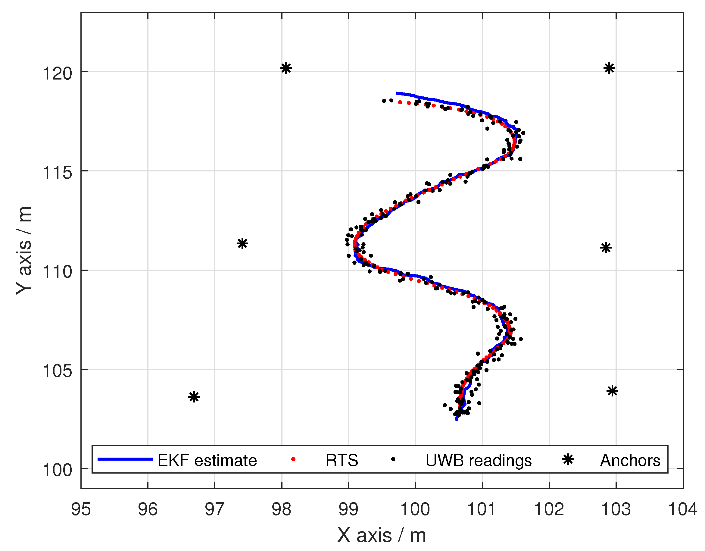
The results of the EKF with a modified, model based sensor measurement variance may be seen in Figure 10. By comparison with the RTS ground truth, this clearly demonstrates that the model based variance used in an EKF is capable of effectively fusing and filtering the states of a UGV.
4.3. Comparison of the Model Based Variance EKF Estimation to That of the Static Variance EKF Estimation
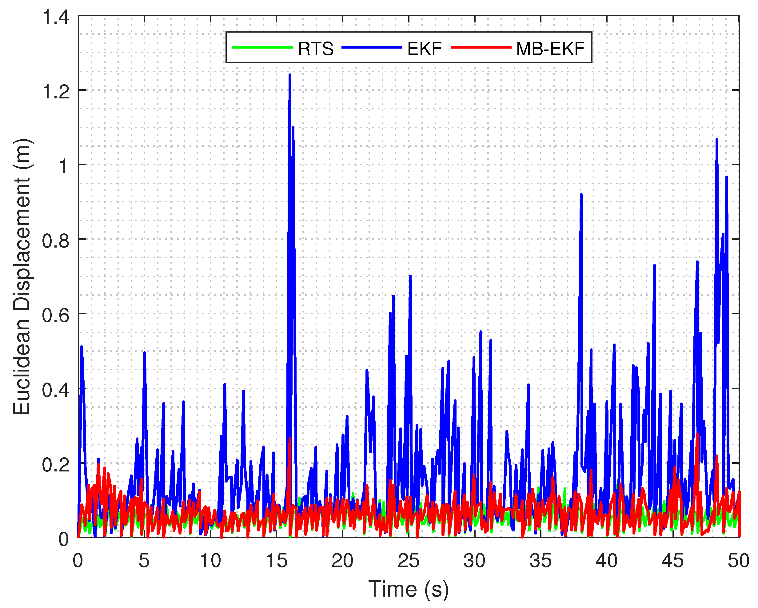
When comparing the conventional EKF demonstrated in the previous works to the model based modification, the tuned process variance was retained for both tests. Process variance tuning remains a constant task in the implementation of an EKF; however, as the model based measurement gives a defined sensor measurement variance, the tuning of this variance is not required. To verify the efficacy of the model based EKF under ideal circumstances, simulated data of a known 0.1 m standard deviation was fabricated and used. As can be seen in Figure 11, the model based EKF allows for a significantly smoothed and representative trajectory estimate, whereas the trajectory estimate of the conventional EKF, although close to the ground truth, is noisy. Testing of the conventional EKF in comparison to the model based EKF using the noisy UWB data taken from the non-ideal UWB platform and environment yielded similar results; however, as expected, due to the inaccurate UWB positional data, sections of the trajectories for both state estimators were off. Moreover, the model based EKF showed a noticeable reduction in the estimated trajectory variance over the conventional formulation. When observing Figure 12, it is evident that the model based EKF estimate provides a significantly more accurate and precise representation of the UGV motion with respect to the point-to-point Euclidean displacement. The main advantage of the model based EKF is its ability to reduce the noise of the estimations generated under non ideal UWB data input, therefore producing a more stable trajectory. The ground truth total displacement acquired from the RTS was calculated at 17.123 m compared to that of the EKF and model based EKF at 53.722 m and 21.1776 m, respectively. From the aforementioned metrics, it is clear that the model based variant of the EKF overall provides a more accurate total displacement estimation. This is primarily the result of the model based EKF possessing the ability to react to noisy and outlier UWB observations compared to that of the standard EKF. This is also observable through the standard deviations of error, where the model based EKF generated a metric of 0.0325 m compared to that of 0.1775 m for the standard EKF. We found that the EKF readings contained an offset to the “right” of the ground truth provided by the RTS. The main focus of the investigation was the improved “smoothness” of the estimate as shown by Figure 12; therefore, for clarity, we left the offset uncorrected. It is also likely that the trajectory used lead to increased liability for yaw errors to have an effect, leading to this offset. As the initial x and y pose of the UGV was taken from the RTS, the estimate uncertainty is low at ±2 mm; however, the heading of the UGV was not measured from a reliable ground truth source; therefore, this initial estimation may not be reliable.
5. Conclusions
In conclusion, this paper demonstrates a method for counteracting increased variance in sensors due to variable factors encountered during operation and presents an alternate method for representing the sensor measurement variance in a state estimation system. We also extend the sensor characterisation methods shown in previous work through the use of surveying grade optical measurement equipment to allow for more comprehensive modeling of localisation sensor variance. This application of a model based variance allows for a reduction in drift and also a reduced tuning period, requiring only the limited tuning of the process variance, in the system formulation presented here.
Future Works
The scope of this project is in the characterisation of the sensor variance as a function of a single dimensional range variable. An important factor for future investigation is the incorporation of the relative pose of the anchor, rover node pair and the effects of the increased dropout rates on localisation. Through the investigation and implementation of a model based variance into an EKF scheme, we have found a definite correlation between the dropout rates of the UWB ranging and the relative pose. In addition to this, a future development of this work is the expansion from two-dimensional, plane fixed systems such as UGVs to three-dimensional systems such as Unmanned Aerial Vehicles (UAVs).
Author Contributions
Conceptualization, H.A.G.P.; Data Curation, H.A.G.P. and B.J.M.; Formal Analysis, H.A.G.P.; Funding Acquisition, F.A.B.; Investigation, H.A.G.P. and B.J.M.; Methodology, H.A.G.P., B.J.M. and F.A.B.; Software, H.A.G.P.; Supervision, F.A.B. and C.M.; Validation, H.A.G.P. and B.J.M.; Visualization, H.A.G.P. and B.J.M.; Writing—Original Draft, H.A.G.P., B.J.M. and F.A.B.; Writing—Review and Editing, H.A.G.P., B.J.M., C.M. and F.A.B.
Funding
This research was funded by Horizon 2020, the EU Research and Innovation programme (Grant No. 660566).
Conflicts of Interest
The authors declare no conflict of interest.
Abbreviations
The following abbreviations are used in this manuscript:
| EKF | Extended Kalman Filter |
| RTS | Robotic Total Station |
| GNSS | Global Navigation Satellite System |
| IMU | Inertial Measurement Unit |
| UWB | Ultra-Wideband |
| UGV | Unmanned Ground Vehicle |
| UAV | Unmanned Aerial Vehicle |
| RFID | RADIO Frequency Identification |
| TOA | Time of Arrival |
| TOF | Time of Flight |
| SMN | Sensor Measurement Noise |
| ROS | Robot Operating System |
References
- Sundvall, P.; Jensfelt, P. Fault detection for mobile robots using redundant positioning systems. In Proceedings of the 2006 IEEE International Conference on Robotics and Automation, 2006, ICRA 2006, Orlando, FL, USA, 15–19 May 2006; pp. 3781–3786. [Google Scholar] [CrossRef]
- Thrun, S.; Burgard, W.; Fox, D. Probabilistic Robotics (Intelligent Robotics and Autonomous Agents); The MIT Press: Cambridge, MA, USA, 2005. [Google Scholar]
- Albrektsen, S.M.; Bryne, T.H.; Johansen, T.A. Phased array radio system aided inertial navigation for unmanned aerial vehicles. In Proceedings of the 2018 IEEE Aerospace Conference, Big Sky, MT, USA, 3–10 March 2018; pp. 1–11. [Google Scholar] [CrossRef]
- The Office of the General Counsel. The Air Navigation Order 2016 and Regulations; The Office of the General Counsel: Washington, DC, USA, 2016.
- Tan, K.M.; Law, C.L. GPS and UWB integration for indoor positioning. In Proceedings of the 2007 6th International Conference on Information, Communications and Signal Processing, ICICS, Singapore, 10–13 December 2007. [Google Scholar] [CrossRef]
- Tiemann, J.; Schweikowski, F.; Wietfeld, C. Design of a UWB indoor-positioning system for UAV navigation in GNSS-denied environments. In Proceedings of the 2015 International Conference on Indoor Positioning and Indoor Navigation, IPIN 2015, Banff, AB, Canada, 13–16 October 2015. [Google Scholar] [CrossRef]
- Vanegas, F.; Gonzalez, F. Enabling UAV navigation with sensor and environmental uncertainty in cluttered and GPS-denied environments. Sensors 2016, 16, 666. [Google Scholar] [CrossRef] [PubMed]
- Das, A.K.; Member, S.; Fierro, R.; Kumar, V.; Member, S.; Ostrowski, J.P.; Spletzer, J.; Taylor, C.J. A Vision-Based Formation Control Framework. IEEE Trans. Robot. Autom. 2002, 18, 813–825. [Google Scholar] [CrossRef]
- Conceição, T.; dos Santos, F.N.; Costa, P.; Moreira, A.P. Robot localization system in a hard outdoor environment. In Advances in Intelligent Systems and Computing; Springer: Cham, Switzerland, 2018; Volume 693, pp. 215–227. [Google Scholar] [CrossRef]
- Chaves, A.N.; Cugnasca, P.S.; Neto, J.J. Adaptive search control applied to Search and Rescue operations using Unmanned Aerial Vehicles (UAVs). IEEE Lat. Am. Trans. 2014, 12, 1278–1283. [Google Scholar] [CrossRef]
- McLoughlin, B.J.; Pointon, H.A.; McLoughlin, J.P.; Shaw, A.; Bezombes, F.A. Uncertainty characterisation of mobile robot localisation techniques using optical surveying grade instruments. Sensors 2018, 18, 2274. [Google Scholar] [CrossRef] [PubMed]
- Masiero, A.; Fissore, F.; Vettore, A.; Masiero, A.; Fissore, F.; Vettore, A. A Low Cost UWB Based Solution for Direct Georeferencing UAV Photogrammetry. Remote Sens. 2017, 9, 414. [Google Scholar] [CrossRef]
- McLoughlin, B.; Cullen, J.; Shaw, A.; Bezombes, F. Towards an Unmanned 3D Mapping System Using UWB Positioning. In Towards Autonomous Robotic Systems. TAROS 2018; Giuliani, M., Assaf, T., Giannaccini, M., Eds.; Lecture Notes in Computer Science; Springer: Cham, Switzerland, 2018; Volume 10965, pp. 416–422. [Google Scholar] [CrossRef]
- Guo, K.; Qiu, Z.; Miao, C.; Zaini, A.H.; Chen, C.L.; Meng, W.; Xie, L. Ultra-Wideband-Based Localization for Quadcopter Navigation. Unmanned Syst. 2016, 4, 23–34. [Google Scholar] [CrossRef]
- Fontana, R.J. Recent system applications of short-pulse ultra-wideband (UWB) technology. IEEE Trans. Microw. Theory Tech. 2004, 52, 2087–2104. [Google Scholar] [CrossRef]
- Liu, H.; Darabi, H.; Banerjee, P.; Liu, J. Survey of wireless indoor positioning techniques and systems. IEEE Trans. Syst. Man Cybern. Part C Appl. Rev. 2007, 37, 1067–1080. [Google Scholar] [CrossRef]
- Gigl, T.; Janssen, G.J.; Dizdarevic, V.; Witrisal, K.; Irahhauten, Z. Analysis of a UWB Indoor Positioning System Based on Received Signal Strength. In Proceedings of the 2007 4th Workshop on Positioning, Navigation and Communication, Hannover, Germany, 22 March 2007; pp. 97–101. [Google Scholar] [CrossRef]
- Arasaratnam, I.; Haykin, S. Cubature kalman filters. IEEE Trans. Autom. Control 2009, 54, 1254–1269. [Google Scholar] [CrossRef]
- Wang, H.; Deng, Z.; Feng, B.; Ma, H.; Xia, Y. An adaptive Kalman filter estimating process noise covariance. Neurocomputing 2017, 223, 12–17. [Google Scholar] [CrossRef]
- Schmitz, G.; Alves, T.; Henriques, R.; Freitas, E.; El’Youssef, E. A simplified approach to motion estimation in a UAV using two filters. IFAC-PapersOnLine 2016, 49, 325–330. [Google Scholar] [CrossRef]
- Kapoor, R.; Ramasamy, S.; Gardi, A.; Sabatini, R. UAV Navigation using Signals of Opportunity in Urban Environments: A Review. Energy Proc. 2017, 110, 377–383. [Google Scholar] [CrossRef]
- Viandier, N.; Nahimana, D.F.; Marais, J.; Duflos, E. GNSS performance enhancement in urban environment based on psuedo-range error model. In Proceedings of the Record—IEEE PLANS, Position Location and Navigation Symposium, Monterey, CA, USA, 5–8 May 2008; pp. 377–382. [Google Scholar] [CrossRef]
- Quigley, M.; Conley, K.; Gerkey, B.; Faust, J.; Foote, T.; Leibs, J.; Wheeler, R.; Ng, A.Y. ROS: An open-source Robot Operating System. In Proceedings of the ICRA Workshop on Open Source Software, Kobe, Japan, 12–17 May 2009; Volume 3, p. 5. [Google Scholar]
- Alarifi, A.; Al-Salman, A.; Alsaleh, M.; Alnafessah, A.; Al-Hadhrami, S.; Al-Ammar, M.A.; Al-Khalifa, H.S. Ultra wideband indoor positioning technologies: Analysis and recent advances. Sensors 2016, 16, 707. [Google Scholar] [CrossRef] [PubMed]
- Pozyx—Centimeter Positioning for Arduino. Available online: https://www.pozyx.io/ (accessed on 21 December 2018).
Figure 1.
Testing room layout.

Figure 2.
Setting the global testing operating frame (a) backsight setup with RTS (b) Unmanned ground testing platform P.E.R.C.I.
Figure 2.
Setting the global testing operating frame (a) backsight setup with RTS (b) Unmanned ground testing platform P.E.R.C.I.

Figure 3.
View of UGV (a) and RTS telescopic view of UWB anchor position (b).

Figure 4.
UWB range sample testing.

Figure 5.
Dynamic UWB range testing with RTS ground truth.

Figure 6.
Dynamic UWB range sample testing.

Figure 7.
Comparison of UWB rover node positioning (a) obscured rover node; (b) simulated un-obscured rover node.
Figure 7.
Comparison of UWB rover node positioning (a) obscured rover node; (b) simulated un-obscured rover node.

Figure 8.
Static UWB range accumulated sample testing.

Figure 9.
Static UWB range sample testing.

Figure 10.
Model-based EKF trajectory using simulated UWB data.

Figure 11.
Comparison of EKF with a generalised variance to an EKF using a model based one, with an obstructed UWB rover node. (a) generalised variance; (b) model based variance.
Figure 11.
Comparison of EKF with a generalised variance to an EKF using a model based one, with an obstructed UWB rover node. (a) generalised variance; (b) model based variance.

Figure 12.
Comparison between Euclidean distance estimations.

© 2019 by the authors. Licensee MDPI, Basel, Switzerland. This article is an open access article distributed under the terms and conditions of the Creative Commons Attribution (CC BY) license (http://creativecommons.org/licenses/by/4.0/).
Share and Cite
MDPI and ACS Style
Pointon, H.A.G.; McLoughlin, B.J.; Matthews, C.; Bezombes, F.A. Towards a Model Based Sensor Measurement Variance Input for Extended Kalman Filter State Estimation. Drones 2019, 3, 19. https://doi.org/10.3390/drones3010019
AMA Style
Pointon HAG, McLoughlin BJ, Matthews C, Bezombes FA. Towards a Model Based Sensor Measurement Variance Input for Extended Kalman Filter State Estimation. Drones. 2019; 3(1):19. https://doi.org/10.3390/drones3010019
Chicago/Turabian StylePointon, Harry A. G., Benjamin J. McLoughlin, Christian Matthews, and Frederic A. Bezombes. 2019. "Towards a Model Based Sensor Measurement Variance Input for Extended Kalman Filter State Estimation" Drones 3, no. 1: 19. https://doi.org/10.3390/drones3010019