
A Method for Forest Canopy Height Inversion Based on UAVSAR and Fourier–Legendre Polynomial—Performance in Different Forest Types


1
College of Forestry, Southwest Forestry University, Kunming 650224, China
2
Forestry 3S Engineering Technology Research Center, Southwest Forestry University, Kunming 650224, China
*
Author to whom correspondence should be addressed.
Drones 2023, 7(3), 152; https://doi.org/10.3390/drones7030152
Submission received: 28 December 2022
/
Revised: 13 February 2023
/
Accepted: 20 February 2023
/
Published: 22 February 2023
(This article belongs to the Special Issue Drone-Based Information Fusion for Agricultural and Forestry Applications)
Abstract
:Mapping forest canopy height at large regional scales is of great importance for the global carbon cycle. Polarized interferometric synthetic aperture radar is an efficient and irreplaceable remote sensing tool. Developing an efficient and accurate method for forest canopy height estimation is an important issue that needs to be addressed urgently. In this paper, we propose a novel four-stage forest height inversion method based on a Fourier–Legendre polynomial (FLP) with reference to the RVoG three-stage method, using the multi-baseline UAVSAR data from the AfriSAR project as the data source. The third-order FLP is used as the vertical structure function, and a small amount of ground phase and LiDAR canopy height is used as the input to solve and fix the FLP coefficients to replace the exponential function in the RVoG three-stage method. The performance of this method was tested in different forest types (mangrove and inland tropical forests). The results show that: (1) in mangroves with homogeneous forest structure, the accuracy based on the four-stage FLP method is better than that of the RVoG three-stage method. For the four-stage FLP method, R2 is 0.82, RMSE is 6.42 m and BIAS is 0.92 m, while the R2 of the RVoG three-stage method is 0.77, RMSE is 7.33 m, and bias is −3.49 m. In inland tropical forests with complex forest structure, the inversion accuracy based on the four-stage FLP method is lower than that of the RVoG three-stage method. The R2 is 0.50, RMSE is 11.54 m, and BIAS is 6.53 m for the four-stage FLP method; the R2 of the RVoG three-stage method is 0.72, RMSE is 8.68 m, and BIAS is 1.67 m. (2) Compared to the RVoG three-stage method, the efficiency of the four-stage FLP method is improved by about tenfold, with the reduction of model parameters. The inversion time of the FLP method in a mangrove forest is 3 min, and that of the RVoG three-stage method is 33 min. In an inland tropical forest, the inversion time of the FLP method is 2.25 min, and that of the RVoG three-stage method is 21 min. With the application of large regional scale data in the future, the method proposed in this study is more efficient when conditions allow.
1. Introduction
Forest height is key information for forest ecosystems, and estimating forest height is a timely and important research topic for improving forest management activities and researching the role of forests as carbon sinks or sources in the global carbon cycle [1]. Synthetic aperture radar (SAR) and laser ranging (LiDAR) are important remote sensing techniques for forest height estimation and have strong penetration capability in forests. Usually, LiDAR can achieve high accuracy forest height estimation [2]. However, few available satellite-based data and the high cost of airborne data acquisition limit its wide application in the field of remote sensing estimation of forest height [3]. Microwave radar is an advanced active remote sensing technology that is less susceptible to climatic factors such as clouds, fog, and solar radiation, allowing for all-weather and large-scale Earth observations [4,5,6].
In microwave remote sensing, polarimetric synthetic aperture radar interferometry (PolInSAR) has been extensively studied in the last two decades and has proven to be an effective tool for forest height estimation because it is sensitive to the vertical structure and physical properties of the scattering medium [7,8,9]. According to microwave theory, it is possible to invert forest height directly from interferograms of ground and volume regimes, which is the simplest application but not very accurate [10,11,12]. Another method is the physical scattering model-based method for forest height estimation [13,14,15], of which the most classical and widely used is the two layer random volume of ground (RVoG) coherence scattering model [16]. In the RVoG model, the forest medium is described as a homogeneous volume layer on the ground, which describes the forest scattering process as a forest volume scattering layer and a ground layer, treating the volume scattering layer as an isotropic homogeneous medium of thickness hv and describing the scattering and absorption losses of electromagnetic waves in it by an average attenuation coefficient σ [8,16,17], which treats the volume coherence as a function of four main parameters: forest height, extinction coefficient, ground to volume amplitude ratio, and ground phase. Based on the RVoG model, Cloude and Papathanassiou [17] first proposed a three-stage algorithm for tree height retrieval, which is simple to implement, time-saving, and widely used to transform PolInSAR measurements into forest parameters.
For PolInSAR data obtained at low frequencies (e.g., L- and P-band), the main scatterers of the forest are massive tree trunks and branches, which are not randomly and homogeneously distributed in the vertical direction. In this case, it is not reasonable to use the homogeneous assumption of the RVoG model to describe the scattering process of the forest. Therefore, related studies have proposed an improved RVoG model [18], an RVoG model with different extinction, and a Gaussian vertical backscattering model as an expression function of the vertical distribution of forest scatterers [19,20,21]. In fact, because of the high complexity of the vertical structure in the forest, it is difficult to accurately express the scattering process of PolInSAR data by a specific function. To solve this problem, the tomographic SAR (TomoSAR) technique was used to estimate the vertical distribution of forest scatterers without relying on any scattering model [22]. However, to ensure, a favorable inversion, a large and homogeneously distributed baseline of SAR images is required, which limits the scope of application of this technique. On this basis, Cloude [23,24,25], and Cloude and Papathanassiou [26] proposed the polarization coherence tomography (PCT) technique to characterize the microwave scattering process based on the Fourier–Legendre (FL) level under the condition that the a priori forest height and surface height are known, which is applicable to both single-baseline and multi-baseline PolInSAR. Ideally, the order of the FLP should be set as high as possible because higher-order FLP can detect the forest’s vertical structure at high resolution. However, in practice, higher order FLP are more sensitive to observation errors, such as temporal decorrelation, signal-to-noise decorrelation, and spatial baseline decorrelation, which may lead to significant estimation bias in FLP model inversion. Previous studies have demonstrated that third-order FLP are sufficient to describe vertical forest structure for biomass estimation [27,28,29]. Because of the direct relationship between forest biomass and forest height, third-order FLP have also been used for forest height inversion. Compared with the RVoG model, the scattering based on the FL level is an approximation to the real forest scene, but the prerequisite is that a priori forest height and phase letter inputs are needed to estimate the FLP coefficients for each pixel cell, which limited the application of the method in forest height estimation. As mentioned in Cloude’s study [25], the FLP coefficients are related to the ground-to-volume magnitude ratio of the polarization channel, which will directly affect the accuracy of the vertical structure function, while previous studies usually assume that the ground-to-volume magnitude ratio of the polarization channel for the volume scattering is close to 0. This assumption holds when the forest structure is homogeneous, and we can use a fixed FLP coefficient to construct the vertical structure function to replace the exponential function of the RVoG model, which not only reduces the model parameters, but also improves the model accuracy. However, the applicability of using fixed FLP coefficients to represent the whole scene when the forest structure varies widely is another question worth exploring.
To answer the above questions, we propose a four-stage forest canopy height inversion method based on FLP. The first and second stages of the RVoG three-stage method were used to solve the ground phase and volume coherence; the third-order FLP was used as the vertical structure function, and a small number of samples from the LiDAR canopy height and ground phase of the RVoG three-stage method were used as input to solve the FLP coefficients to construct the vertical structure function for forest canopy height inversion using the look-up table method. The performance of this method in mangrove and inland tropical forests was tested to verify the potential and conditions of using the fixed FLP coefficients method for canopy height estimation in different types of forests. The purpose of this study is to develop an accurate and efficient forest height inversion method at the regional scale, using FLP and fixed polynomial coefficients to replace the exponential function in the RVoG three-stage method. Currently, a large number of laser samples have been acquired by GEDI and ICEsat-2. With the arrival of TanDEM-L and BIOMASS satellites and the NISAR program, efficient monitoring of global forest ecosystems will be further improved.
2. Materials and Methods
2.1. Study Area and Data
In this study, both the airborne multi-baseline UAVSAR data and the LiDAR-RH100 validation data are derived from the publicly available datasets of the AfriSAR project (see Table 1). In 2016, NASA, ESA and the Gabonese Space Agency collaborated on the AfriSAR campaign, where NASA’s unmanned aerial vehicle synthetic aperture radar (UAVSAR) and airborne LiDAR sensors acquired L-band multi-baseline fully polarized PolInSAR data and full-waveform LVIS LiDAR datasets, respectively, which is part of NASA-ESA’s BIOMASS, GEDI, and NISAR calibration and validation activities. The UAVSAR dataset is processed for polarization calibration, baseline fine coregistered and spectral filtering, and is provided as a single-look complex [30], with each track containing SLC data for four polarization channels (HH, HV, VH and VV). In this paper, Lope and Pongara, located in the Gabonese Republic on the west coast of Africa, were selected as the test areas (see Figure 1), where the forest type of Lope is an inland tropical forest and Pongara is a mangrove forest. The number of tracks in the Lope test area is eight, and the number of tracks in Pongara is five. In this study, 2 × 8 SLC data were used, and the PD coherence optimization algorithm [31] was used to calculate the complex coherence under different baseline combinations for forest canopy height inversion, which was geocoded at 25 m resolution size.
The relative height variable RH100 derived from LVIS LiDAR data was used as the true value to evaluate the accuracy of canopy height estimation. In this study, the RH100 canopy height product used was from the Oak Ridge National Laboratory (ORNL) Distributed Active Archive Center (DAAC), with a spatial resolution of 25 m [32].
2.2. RVoG Coherence Scattering Model
The RVoG coherence scattering model describes the forest scattering process as a forest volume scattering layer and a ground layer that cannot be penetrated, assumes the volume scattering as an isotropic homogeneous medium of thickness hv, and uses an extinction coefficient σ to describe the scattering and absorption losses of electromagnetic waves in the volume layer [8,13,16]. The theory is as follows:
where m(ω) is the effective ground-to-volume amplitude ratio, φ0 indicates the ground phase, and γv indicates the “pure” volume coherence, expressed as Equation (2).
where σ is the average extinction coefficient, hv is the forest height, kz is the vertical effective wave number, kz denotes the phase change corresponding to a height change of 1 m. The height of ambiguity (hoa) denotes the interference phase change of 2π producing a height change, R is the slant distance, B⊥ is the vertical baseline length, and n depends on the acquisition mode of the radar image [33].
2.3. Baseline Selection Method
In the RVoG model, the distribution of the complex coherence points under ideal conditions is approximately elliptical. In this paper, multiple baseline datasets are used, so the most suitable pair of baseline combinations from multiple baselines can be selected for forest canopy height inversion, and the best combination of baselines that fits the assumptions of the RVoG model is chosen based on the degree of separation of the complex coherence and the coherence magnitude information. In this study, baselines were selected using the PROD method (Equation (3)), which uses the product of the coherence separation and the average coherence amplitude as an evaluation index, and the baseline combination was obtained by baseline selection when the PROD value within each observation unit was maximum [34,35,36].
where γl denotes the complex coherence near the surface, γh denotes the complex coherence near the top of the canopy.
2.4. RVOG Three-Stage Method
The three-stage forest height inversion method, proposed by Cloude and Papathanassiou [13], solves the ground phase by fitting a coherence line and uses the look-up table method for forest height inversion in a three-stage process.
First stage: Fitting the coherence line. In this study, the PD coherence optimization algorithm is used to calculate the complex coherence under different baseline combinations [36], and the interferometric complex coherence (γh, γl) under the best baseline combination is obtained by baseline selection, and fitting the coherence line where the two coherence points are located, which intersects with the unit circle to obtain two potential ground phase points (Figure 2a).
The second stage: Determining the ground phase φ0 from the two potential ground phases. The complex coherence farthest from the ground phase is selected as the volume scattering complex coherence (Figure 2b).
The third stage: The estimation of forest height (hv) and extinction coefficient (σ). A two-dimensional look-up table is created (LUT) by setting reasonable hv and σ according to the relationship between γv and (hv and σ) in Equation (2), and the inversion process is used to search the forest height (hv) and extinction coefficient (σ) corresponding to the γv with the smallest distance from γh in the look-up table (Equation (4)).
2.5. FLPMethod
This method represents the interferometric complex coherence as the integration of the vertical structure function in the height direction and expands this function in the form of an FL order, which is then solved for the FLP coefficients based on the a priori forest height and topographic phase. Based on the RVoG model, the pure volume coherence is expanded by the FL order [25], expressed as Equation (5). Previous studies have demonstrated that third-order FLP are sufficient to describe vertical forest structure for biomass estimation [27,28,29]. Because of the direct relationship between forest biomass and forest height, third-order FLP have also been used for forest height inversion.
where an is the Legendre coefficient. f0, f1, f2 denotes the i-th order FLP.
2.6. Fixed FLP Coefficients
In the study of cloud [13], it is mentioned that the FLP coefficients are related to the ground-to-volume magnitude ratio of the polarization channel, as shown in Figure 3, where the FLP coefficients change with the ground-to-volume magnitude ratio. Previous studies have usually assumed that the ground-to-volume magnitude ratio of complex coherence dominated by volume scattering is 0. When the structure of forest conditions changes greatly, differences in forest cover within different observation units can lead to inconsistent ground-to-volume magnitude ratios, in which case the use of fixed FLP coefficients to represent the whole study area is subject to error. We designed a four-stage forest height inversion method to test this hypothesis using fixed FLP coefficients.
2.7. A Novel Four-Stage Forest Canopy Height Inversion Method Based on FLP
Since the FLP is mainly used for tomographic techniques, the solution of the polynomial coefficients requires an a priori forest height and ground phase corresponding to each pixel cell, which can limit the extension of the method. Therefore, we propose solving and fixing the FLP coefficients representing the whole scene by a small number of training samples and comparing this approach’s applicability in different forests.
The four-stage forest canopy height inversion method based on the FLP, which is based on the RVoG three-stage method, uses a third-order FLP as the vertical structure function of forest height and is solved by the following procedure.
First and second stages: solving the ground phase and volume coherence using the first and second stages of the RVoG three-stage method.
Third stage: a limited amount of a priori data of ground phase φ0 and RH100 is used as input to solve the FLP coefficients a10 and a20 using nonlinear least squares (Equation (6)) and applied to the whole experimental area to obtain the vertical structure function expressions.
γ(w) denotes the complex coherence of the arbitrary polarization channel.
Fourth stage: Inversion the forest height (hv) using the look-up table method. According to Equation (5), a reasonable range of forest height hv is set as input to construct a look-up table. From Equation (7), it can be found that the method no longer relies on the extinction coefficient; the unknowns become only hv.
3. Results
To validate the four-stage forest canopy height inversion method based on FL and its applicability, two different forest types were selected for validation in this study, the first being a mangrove forest with a homogeneous structure and the second being an inland tropical forest with a complex structure.
3.1. Estimation Results in Mangroves
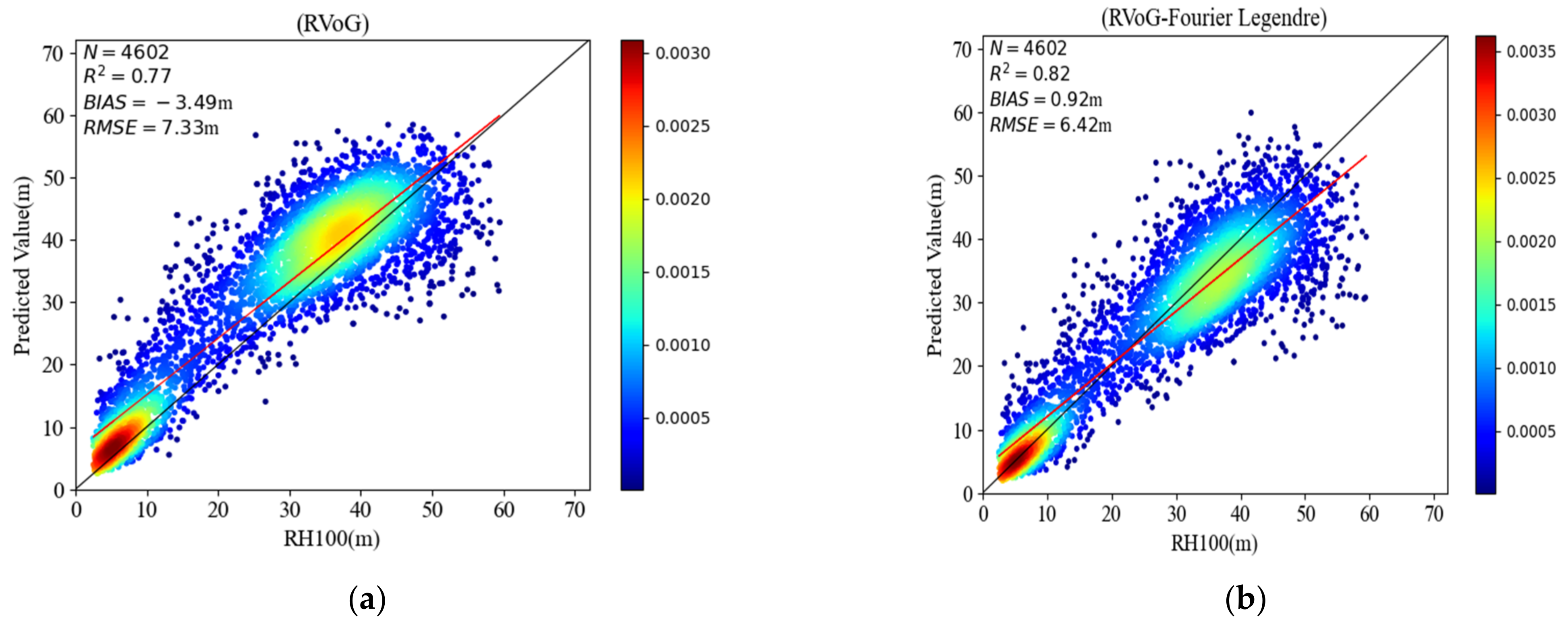
In the mangrove test area of Pongara, 4602 sample points of LIDAR canopy height RH100 were selected to validate the inversion results, and the results are shown in Figure 4 and Figure 5. The R2 of the RVoG three-stage method inversion results is 0.77, the RMSE is 7.33 m, and the BIAS is −3.49 m. The scatter plot (Figure 4a) shows that the sample points show an overall overestimation, the fitted trend line is above the 1:1 line, and a small number of sample points are underestimated when the forest height is greater than 40 m. The inversion results (Figure 5a,d) also show that the forest canopy height values based on the RVoG three-stage method are greater than RH100 overall. The inversion accuracy based on the four-stage FLP method was better than that of the RVoG model, and the R2 is 0.82, the RMSE is 6.42 m, and the BIAS is 0.92 m. From the scatter plot (Figure 4b), it was found that the overestimation phenomenon was improved compared with the RVoG model, and the fitted trend line was closer to the 1:1 line. However, there is still a small number of samples with underestimation when the forest height is greater than 45 m. From the inversion results (Figure 5b,e), it can be found that the inversion results are closer to RH100 based on the four-stage FLP method.
3.2. Estimation Results in Inland Forests
In the Lope test area of the inland tropical forest, the inversion results were verified with 6436 samples of LIDAR canopy height RH100. The results are shown in Figure 6 and Figure 7. The R2 of the inversion results in the RVoG three-stage method is 0.72, the RMSE is 8.68 m, and the BIAS is 1.67 m. From the scatter plot (Figure 6a), it is found that the overestimation phenomenon is obvious when the forest height is lower than 25 m, and the underestimation phenomenon is more significant when the forest height is greater than 35 m, and this phenomenon can also be seen in the inversion result Figure 5a,d. The inversion accuracy based on the four-stage FLP method is lower than that of the RVoG model; the R2 is 0.50, the RMSE is 11.54 m, and the BIAS is 6.53 m. From the scatter plot (Figure 6a), it is found that when the forest height is lower than 20 m, there is still overestimation of lower forests, which is consistent with the inversion results of the RVoG three-stage method, and the underestimation is more obvious when the forest height is higher than 25 m, and the underestimation is more serious than that of the RVoG three-stage method, which is also shown in the inversion results in Figure 5b,e. Moreover, a small number of outlier sample points exists in the inversion results of both methods.
3.3. Model Efficiency Comparison
In constructing the look-up table for forest height estimation, the input parameter of the four-stage FLP method is forest height hv, but the RVoG three-stage method is forest height hv and extinction coefficient σ. Therefore, the solution speed of the FLP method is greatly improved with the reduction of model parameters (Figure 8), and the inversion elapsed time is significantly reduced. The inversion time of the FL method in the mangrove forest is 3 min, and that of the RVoG three-stage method is 33 min, while that of the FL method in the inland tropical forest is 2.25 min, and that of the RVoG three-stage method is 21 min. The efficiency is improved by about tenfold.
4. Discussion
In the mangrove forest, the inversion results based on the four-stage FLP method were better than those of the RVoG three-stage method, but in the inland tropical forest, the inversion results of the RVoG three-stage method were better than those of the four-stage FLP method (Table 2). We will analyze the reasons for the difference in results between the two forest types from the following aspects.
4.1. Differences in Forest Types
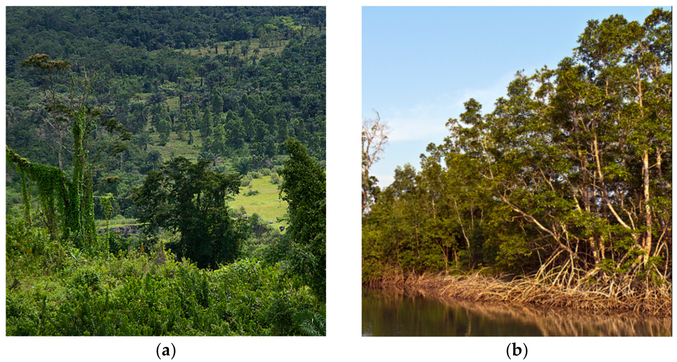
As mentioned in the cloud [13] study, the FLP coefficients are related to the ground-to-volume magnitude ratio of the polarization channel. According to the scattering mechanism of SAR, since the ground-to-volume magnitude ratio is close to 0 for the complex coherence γH dominated by volume scattering, it can be assumed that the ground-to-volume magnitude ratio is consistent in a structurally homogeneous forest, and thus a fixed FLP factor can be used to represent the whole study area. According to Figure 9, it can be seen that mangrove forests are broadleaf forests, the structure in mangrove forests is more homogeneous, in this area, the canopy cover is larger, and there is no other vegetation on the forest ground surface, in which case the condition is valid for fixed FLP coefficients. However, in the inland tropical forest, the tree species composition is diverse, and the underground vegetation is complex. In the scatter plot in Figure 6a and Figure 9a, it can be seen that the forest height in Lope shows a polarization phenomenon, with more tall and low forests. Under the condition of low forest cover, the contribution of surface scattering is larger, and the dry surface in the inland forest reflects electromagnetic waves more strongly compared with the mangrove forest, so the assumption that the ground-to-volume magnitude ratio of the whole study area is 0 is not fully valid; therefore, it is not feasible to use a fixed FLP coefficient in the inland forest, which leads to the FLP method having a lower inversion accuracy. In the next step of the study, the performance of this method in other forest types is explored to draw a more definite conclusion.
4.2. Impact of the Baseline Selection Method
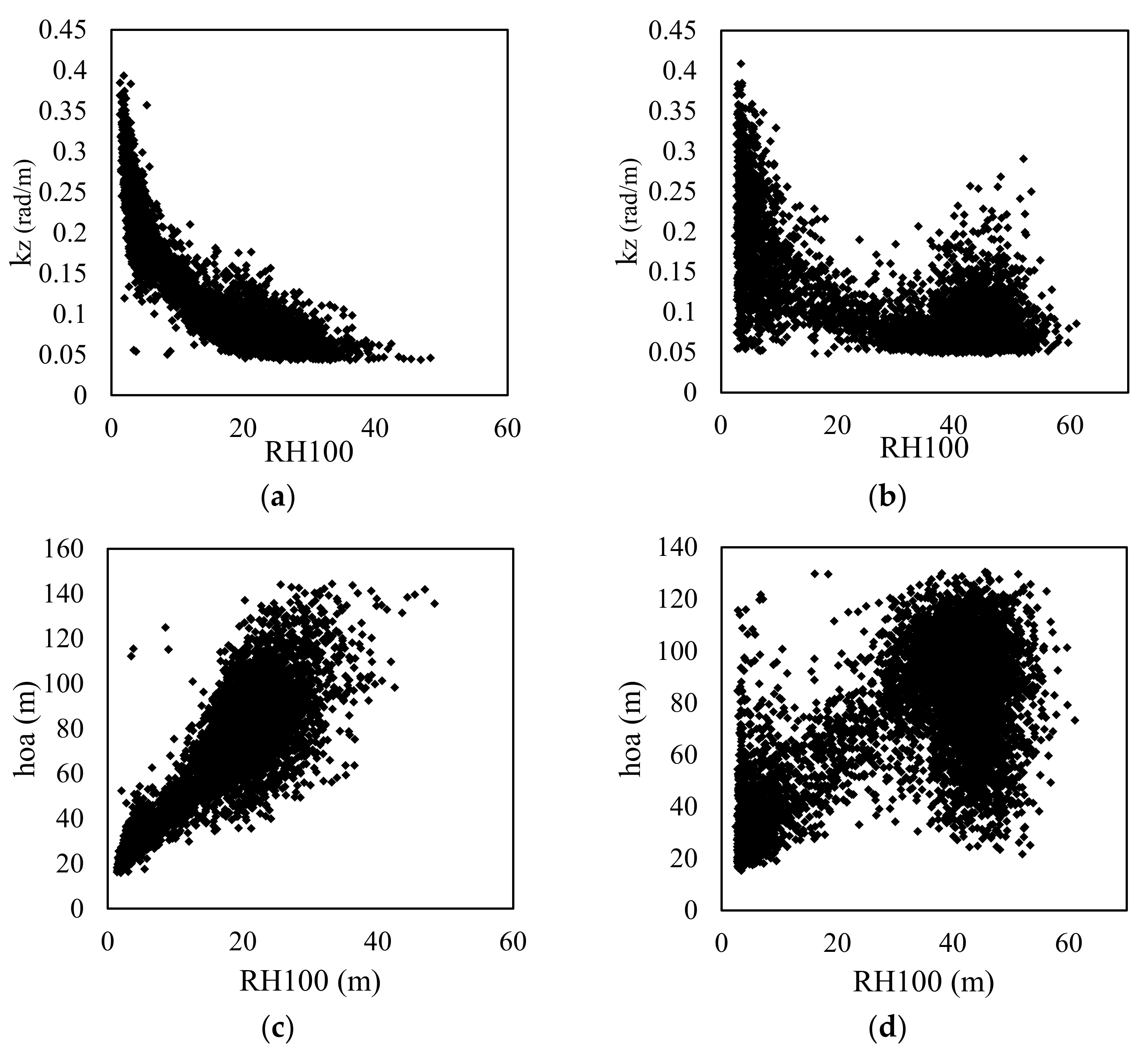
Another important parameter related to forest canopy height inversion is the vertical effective wave number kz and the 2π height of ambiguity (hoa). Long baselines produce smaller ambiguity heights corresponding to larger kz, which are sensitive to low forests, and short baselines produce larger ambiguity heights and smaller kz. Kugler and Schlund’s study shows that baseline size has an important effect on forest height inversion [33,37], with short baselines reducing sensitivity to forest height and long baselines reducing coherence and thus limiting forest height inversion. Previous studies have shown that when the product of forest height and vertical wave number is less than hoa (kz × hv < hoa), the inversion results are more accurate, and either too large or too small values of kz would increase the interference of decorrelation [38,39], while the spatial baseline is an important parameter for determining kz. Despite our study’s use of multi-baseline PolInSAR and baseline selection, it was impossible to fully overcome the baseline effects. From the scatter plots Figure 10a,c, it can be seen that Hoa increases with forest height in mangrove forests, which is consistent with the requirement of forest height on hoa size. However, in the inland forest, the hoa is much larger than the forest height when the forest height is less than 20 m. Moreover, when the forest height is larger than 30 m, many sample points correspond to Hoa much smaller than the forest height (Figure 10b,d), so the overestimation and underestimation are more serious in the canopy height inversion results of the inland forest. As mentioned above, the forest structure in mangroves is homogeneous and closer to the RVoG model hypothesis, and the baseline selection results are more reasonable, while the structural composition of inland tropical forests is complex, with more interference factors, and relying only on the product of coherence separation and average coherence amplitude as the baseline selection criteria does not reflect the true forest height information, which was also verified in the study of Denbina [35], and the optimization and improvement of baseline selection methods in the next study is also a new research problem.
4.3. The Impact of Temporal Decorrelation
There is a temporal interval in the acquisition of airborne SAR data, and the mangrove area in the Pongara experiment area is more affected by dielectric constants such as wind and water. Hence the effect of temporal decorrelation is more obvious. Lee [40,41,42] found that temporal decorrelation reduced the coherence coefficient and increased the coherence phase volatility in vegetation areas. Moreover, the effect of temporal decorrelation is more severe in low vegetation areas, which caused the higher height of the center of volume coherence phase, resulting in overestimation of low vegetation, which is a common problem in PolInSAR forest height estimation. It was consistent with the findings of Lee [42], but our study showed that the FLP method could improve the overestimation of lower forests.
4.4. The Impact of Microwave Penetration
PolInSAR is an active remote sensing method, and the electromagnetic wave signals penetrate the forest to a certain extent. Compared with X-band and C-band, the larger wavelength makes the L-band SAR signals penetrate the forest more deeply, causing the interference phase center to be located at the top lower part of the canopy [16,43,44]. The scatter plots from both test areas in this paper show that the overestimation is more obvious at higher forest height; the use of microwave penetration to improve this defect may be considered in future studies.
4.5. Limitations of This Method
In this study, we propose a method to improve forest canopy height estimation using FLP instead of the vertical structure function of the RVoG model, which presupposes a homogeneous forest structure and requires the support of a priori forest height data, which is an important factor limiting the extension of this method, and still cannot overcome the overestimation problem in low and sparse vegetation areas. The next research question is how to improve the usability of this method in complex structured forests.
5. Conclusions
The PolInSAR technique is an important remote sensing tool in forest height estimation, and among the current PolInSAR-based forest height estimation methods, the RVoG three-stage method is the most classical and widely used method. However, it is difficult to accurately express the scattering process of the PolInSAR signal by a specific function due to the high complexity of the vertical structure of the forest. To solve this problem, a third-order FLP was used to replace the exponential function in the RVoG three-stage method, and a small number of LiDAR height samples was used to solve the coefficients of the polynomial to construct a four-stage forest height inversion method. The results show that the inversion accuracy of the four-stage FLP-based method is higher in mangroves with homogeneous forest structures, but this conclusion is reversed in the complex structure of inland tropical forests, and the applicability conditions of the two models are different. In the four-stage FLP method, the model inversion time is greatly reduced, and the efficiency is improved by about tenfold compared with the RVoG three-stage method. With the realization of TanDEM-L and BIOMASS satellites and the NISAR program, it is essential to develop an efficient forest height inversion method to obtain forest structure parameters on a global scale.
Author Contributions
H.L. designed the experiments, completed the data analysis, and wrote the paper; C.Y. provided important guidance for the experimental design, data analysis, and writing of the paper; H.Y. assisted with the experiments; N.W. assisted with data processing; and S.C. assisted with the development of the graphs. All authors have read and agreed to the published version of the manuscript.
Funding
This research was funded by the Major Science and Technology Special Project of Yunnan Provincial Science and Technology Department “Forest Resources Digital Development and Application in Yunnan” (Grant No. 202002AA100007-015); the National Natural Science Foundation of China “Multi-frequency SAR polarized interferometric data for forest tree height inversion” (Grant No. 42061072); and the Scientific Research Fund Project of Yunnan Provincial Education Department “Forest height inversion from starborne microwave data TanDEM-X combined with topographic data” (Grant No. 2022Y579).
Data Availability Statement
UAVSAR data and LiDAR-RH100 were obtained from NASA’s Oak Ridge National Laboratory Biogeochemical Dynamics Distributed Active Archive Center (https://daac.ornl.gov/cgi-bin/dataset_lister.pl?p=38 (accessed on 19 October 2021)) and Jet Propulsion Laboratory (https://uavsar.jpl.nasa.gov (accessed on 24 December 2021)).
Acknowledgments
Thanks to NASA for providing all the publicly available free datasets to support this work.
Conflicts of Interest
No conflict of interest exists in association with the submission of this manuscript, and the manuscript has been approved for publication by all authors.
References
- Bonan, G.B. Forests and Climate Change: Forcings, Feedbacks, and the Climate Benefits of Forests. Science 2008, 320, 1444–1449. [Google Scholar] [CrossRef] [PubMed] [Green Version]
- Sexton, J.O.; Bax, T.; Siqueira, P.; Swenson, J.J.; Hensley, S. A comparison of lidar, radar, andfield measurements of canopy height in pine and hardwood forests of southeastern North America. Forest Ecol. Manag. 2009, 257, 1136–1147. [Google Scholar] [CrossRef]
- Qi, W.; Lee, S.K.; Hancock, S.; Luthcke, S.; Tang, H.; Armston, J.; Dubayah, R. Improved forest height estimation by fusion of simulated GEDI Lidar data and TanDEM-X InSAR data. Remote Sens. Environ. 2019, 221, 621–634. [Google Scholar] [CrossRef] [Green Version]
- Sinha, S.; Jeganathan, C.; Sharma, L.K.; Nathawat, M.S. A review of radar remote sensing for biomass estimation. Int. J. Environ. Sci. Technol. 2015, 12, 1779–1792. [Google Scholar] [CrossRef] [Green Version]
- Soja, M.J.; Quegan, S.; D’Alessandro, M.M.; Banda, F.; Scipal, K.; Tebaldini, S.; Ulander, L.M.H. Mapping above-ground biomass in tropical forests with ground-cancelled P-band SAR and limited reference data. Remote Sens. Environ. 2021, 253, 112153. [Google Scholar] [CrossRef]
- Vafaei, S.; Soosani, J.; Adeli, K.; Fadaei, H.; Naghavi, H.; Pham, T.D.; Bui, D.T. Improving accuracy estimation of forest aboveground biomass based on incorporation of ALOS-2 PALSAR-2 and Sentinel-2A imagery and machine learning: A case study of the Hyrcanian Forest area (Iran). Remote Sens. 2018, 10, 172. [Google Scholar] [CrossRef] [Green Version]
- Cloude, S.R.; Papathanssiou, K.P. Polarimetric optimization in radar interferometry. Electron. Lett. 1997, 33, 1176–1178. [Google Scholar] [CrossRef]
- Papathanassiou, K.; Cloude, S.R. Single-baseline polarimetric SAR interferometry. IEEE Trans. Geosci. Remote Sens. 2001, 39, 2352–2363. [Google Scholar] [CrossRef] [Green Version]
- Cai, H.; Zou, B.; Lin, M. Parameter inversion model base on PolInSAR images. In Proceedings of the Asian and Pacific Conference on Synthetic Aperture Radar (APSAR-2007), Huangshan, China, 5–9 November 2007. [Google Scholar]
- Neumanm, M.; Famil, L.F.; Reigber, A. Estimation of forest structure, ground and canopy layer characteristics from multi-baseline polarimetric interferometric SAR data. IEEE Trans. Geosci. Remote Sens. 2010, 48, 1086–1103. [Google Scholar] [CrossRef] [Green Version]
- Varvia, P.; Lahivaara, T.; Maltamo, M.; Packalen, P.; Seppanen, A. Gaussian Process Regression for Forest Attribute Estimation from Airborne Laser Scanning Data. IEEE Trans. Geosci. Remote Sens. 2019, 57, 3361–3369. [Google Scholar] [CrossRef] [Green Version]
- Thieu, H.C.; Pham, M.N.; Le, V.N. Forest parameters inversion by mean coherence set from single-baseline polinsar data. Adv. Space Res. 2021, 68, 2804–2818. [Google Scholar] [CrossRef]
- Cloude, S.R.; Papathanassiou, K.P. Polarimetric SAR interferometry. IEEE Trans. Geosci. Remote Sens. 1998, 36, 1551–1565. [Google Scholar] [CrossRef]
- Tayebe, M.; Maghsoudi, Y.; Zoej, M.J.V. A Volume Optimization Method to Improve the Three-Stage Inversion Algorithm for Forest Height Estimation Using PolInSAR Data. IEEE Geosci. Remote Sens. Lett. 2018, 15, 1214–1218. [Google Scholar]
- Cuong, T.H.; Nghia, P.M.; Minh, T.X.; Le, V.N.; Dang, C.H. An improved volume coherence optimization method for forest height estimation using PolInSAR images. In Proceedings of the IEEE International Conference on Recent Advances in Signal Processing, Telecommunications & Computing (SigTelCom2019), Hanoi, Vietnam, 21–22 March 2019. [Google Scholar]
- Treuhaft, R.N.; Moghaddam, M.; van Zyl, J.J. Vegetation characteristics and underlying topography from interferometric radar. Radio Sci. 1996, 31, 1449–1485. [Google Scholar] [CrossRef]
- Cloude, S.R.; Papathanassiou, K.P. Three-stage inversion process for polarimetric SAR interferometry. IEE Proc.-Radar Sonar Navig. 2003, 150, 125–134. [Google Scholar] [CrossRef] [Green Version]
- Cloude, S.R.; Woodhouse, I.H.; Hope, J.; Minguez, S.; Osborne, P.; Wright, G. The Glen Affric Project: Forrest mapping using dual baseline polarimetric radar interferometry. In Proceedings of the 3rd International Symposium on Retrieval of Bio- and Geophysical Parameters from SAR Data for Land Applications, Sheffield, UK, 11–14 September 2001. [Google Scholar]
- Garestier, F.; Le, T.T. Forest modeling for height inversion using single-baseline InSAR/Pol-InSAR data. IEEE Trans. Geosci. Remote Sens. 2010, 48, 1528–1539. [Google Scholar] [CrossRef]
- Fu, W.; Guo, H.; Song, P.; Tian, B.; Li, X.; Sun, Z. Combination of PolInSAR and LiDAR techniques for forest height estimation. IEEE Geosci. Remote Sens. Lett. 2017, 14, 1218–1222. [Google Scholar] [CrossRef]
- Fu, H.; Wang, C.; Zhu, J.; Xie, Q.; Zhang, B. Estimation of pine forest height and underlying DEM using multi-baseline P-band PolInSAR data. Remote Sens. 2016, 8, 820. [Google Scholar] [CrossRef] [Green Version]
- Nannini, M.; Scheiber, R.; Moreira, A. Estimation of the minimum number of tracks for SAR tomography. IEEE Trans. Geosci. Remote Sens. 2009, 47, 531–543. [Google Scholar] [CrossRef]
- Cloude, S.R. Polarization coherence tomography. Radio Sci. 2006, 41, 1113–1114. [Google Scholar] [CrossRef]
- Cloude, S.R. Dual-baseline coherence tomography. IEEE Geosci. Remote Sens. Lett. 2007, 41, 127–131. [Google Scholar] [CrossRef]
- Cloude, S.R. Polarisation Applications in Remote Sensing; Oxford University Press: New York, NY, USA, 2009. [Google Scholar]
- Cloude, S.R.; Papathanassiou, K.P. Forest vertical structure estimation using coherence tomography. In Proceedings of the IEEE International Geoscience and Remote Sensing Symposium IGARSS, Boston, MA, USA, 7–11 July 2008. [Google Scholar]
- Caicoya, A.T.; Kugler, F.; Papathanassiou, K.; Biber, P.; Pretzsch, H. Biomass estimation as a function of vertical forest structure and forest height—Potential and limitations for Radar Remote Sensing. In Proceedings of the European Conference on Synthetic Aperture Radar (EUSAR), Aachen, Germany, 7–10 June 2010. [Google Scholar]
- Nafiseh, G.; Valentyn, T.; Alfred, S. A modified model for estimating tree height from polinsar with compensation for temporal decorrelation. Int. J. Appl. Earth Obs. Geoinf. 2018, 73, 313–322. [Google Scholar]
- Zhang, B.; Fu, H.; Zhu, J.; Peng, X.; Xie, Q.; Lin, D.; Liu, Z. A multibaseline polinsar forest height inversion model based on fourier–legendre polynomial. IEEE Geosci. Remote Sens. Lett. 2021, 18, 687–691. [Google Scholar] [CrossRef]
- Fore, A.G.; Chapman, B.D.; Hawkins, B.P.; Hensley, S.; Jones, C.E.; Michel, T.R.; Muellerschoen, R.J. UAVSAR polarimetric calibration. IEEE Trans. Geosci. Remote Sens. 2015, 53, 3481–3491. [Google Scholar] [CrossRef]
- Xie, Q.H.; Wang, C.C.; Zhu, J.J.; Fu, H.Q. Forest height inversion by combining S-RVOG model with terrain factor and PD coherence optimization. Acta Geod. Et Cartogr. Sinica. 2015, 44, 686. [Google Scholar]
- Armston, J.; Tang, H.; Hancock, S.; Marselis, S.; Duncanson, L.; Kellner, J.; Hofton, M.; Blair, J.; Fatoyinbo, T.; Dubayah, R. Forest biomass estimation over three distinct forest types using TanDEM-X InSAR data and simulated GEDI lidar data. Remote Sens. Environ. 2019, 232, 111283. [Google Scholar]
- Kugler, F.; Schulze, D.; Hajnsek Pretzsch, H.; Papathanassiou, K.P. TanDEM-X Pol-InSAR performance for forest height estimation. IEEE Trans. Geosci. Remote Sens. 2014, 52, 6404–6422. [Google Scholar] [CrossRef]
- Lee, S.K.; Kugler, F.; Papathanassiou, K.; Hajnsek, I. Multibaseline polarimetric SAR interferometry forest height inversion approaches. In Proceedings of the ESA POLinSAR Workshop, Frascati, Italy, 24–28 January 2011. [Google Scholar]
- Luo, H.B.; Zhu, B.D.; Yue, C.R.; Wang, N. Forest Canopy Height Inversion Based On Airborne Multi-Baseline PolInSAR. J. Geomat. 2022, 48, 1–7. [Google Scholar]
- Denbina, M.; Simard, M.; Hawkins, B. Forest Height Estimation Using Multibaseline PolInSAR and Sparse Lidar Data Fusion. IEEE J. Sel. Top. Appl. Earth Obs. Remote Sens. 2018, 11, 3415–3433. [Google Scholar] [CrossRef]
- Liao, Z.; He, B.; van Dijk, A.I.; Bai, X.; Quan, X. The impacts of spatial baseline on forest canopy height model and digital terrain model retrieval using P-band PolInSAR data. Remote Sens. Environ. 2018, 210, 403–421. [Google Scholar] [CrossRef]
- Chen, H.; Cloude, S.R.; Goodenough, D.G.; Hill, D.A.; Nesdoly, A. Radar forest height estimation in mountainous terrain using Tandem-X coherence data. IEEE J. Sel. Top. Appl. Earth Obs. Remote Sens. 2018, 11, 3443–3452. [Google Scholar] [CrossRef]
- Du, K.; Lin, H.; Wang, G.; Long, J.; Li, J.; Liu, Z. The Impact of Vertical Wavenumber on Forest Height Inversion by PolInSAR. In Proceedings of the 2018 Fifth International Workshop on Earth Observation and Remote Sensing Applications (EORSA), Xi’an, China, 18–20 June 2018. [Google Scholar]
- Lee, S.K.; Kugler, F.; Hajnsek, I.; Papathanassiou, K. The impact of temporal decorrelation over forest terrain in polarimetric SAR interferometry. In Proceedings of the International Workshop on Applications of Polarimetry and Polarimetric Interferometry (Pol-InSAR), ESA, Frascati, Italy, 26–30 January 2009. [Google Scholar]
- Lee, S.K.; Kugler, F.; Papathanassiou, K.; Moreira, A. Forest height estimation by means of Pol-InSAR limitations posed by temporal decorrelation. In Proceedings of the 11th ALOS Kyoto & Carbon Initiative, Tsukuba, Japan, 28 December 2009. [Google Scholar]
- Lee, S.-K.; Kugler, F.; Papathanassiou, K.P.; Hajnsek, I. Quantifying temporal decorrelation over boreal forest at L-and P-band. In Proceedings of the 7th European Conference on VDE, Friedrichshafen, Germany, 2–5 June 2008. [Google Scholar]
- Dall, J. InSAR elevation bias caused by penetration into uniform volumes. IEEE Trans. Geosci. Remote Sens. 2007, 45, 2319–2324. [Google Scholar] [CrossRef] [Green Version]
- Schlund, M.; Baron, D.; Magdon, P.; Erasmi, S. Canopy penetration depth estimation with TanDEM-X and its compensation in temperate forests. ISPRS J. Photogramm. Remote Sens. 2019, 147, 232–241. [Google Scholar] [CrossRef]
Figure 1.
Location of the test area.

Figure 2.
RVoG three-stage method solution schematic, (a) indicates the first stage, (b) indicates the second stage.
Figure 2.
RVoG three-stage method solution schematic, (a) indicates the first stage, (b) indicates the second stage.

Figure 3.
Schematic representation of the relationship between the FLP coefficients and the ground-to-volume magnitude ratio (Figure cited in reference [25]).
Figure 3.
Schematic representation of the relationship between the FLP coefficients and the ground-to-volume magnitude ratio (Figure cited in reference [25]).

Figure 4.
Scatterplot of validation results for the Pongara test area: (a) is the RVoG method, (b) is the FLP method (black line indicates 1:1 line, red line is the fitted trend line of the scatter plot).
Figure 4.
Scatterplot of validation results for the Pongara test area: (a) is the RVoG method, (b) is the FLP method (black line indicates 1:1 line, red line is the fitted trend line of the scatter plot).

Figure 5.
Forest canopy height inversion results of the Pongara test area: (a) is the inversion result of the RVoG three-stage method, (b) is the inversion result of the FL four-stage method, (c) is the LIDAR canopy height, and (d,e) are the local inversion results of the RVoG and FL methods, respectively.

Figure 6.
Scatterplot of validation results for the Lope test area: (a) is the RVoG method, (b) is the FLP method (black line indicates 1:1 line, red line is the fitted trend line of the scatter plot).
Figure 6.
Scatterplot of validation results for the Lope test area: (a) is the RVoG method, (b) is the FLP method (black line indicates 1:1 line, red line is the fitted trend line of the scatter plot).

Figure 7.
Forest canopy height inversion results of the Lope test area: (a) is the inversion result of the RVoG three-stage method, (b) is the inversion result of the FL four-stage method, (c) is the LIDAR canopy height, and (d,e) are the local inversion results of the RVoG and FL methods, respectively.

Figure 8.
Comparison of inversion efficiency for different methods.

Figure 9.
Schematic representation of different forest scenes of different forest types: (a) is mangrove and (b) is inland tropical forests.
Figure 9.
Schematic representation of different forest scenes of different forest types: (a) is mangrove and (b) is inland tropical forests.

Figure 10.
kz and hoa after baseline selection for different test areas: (a,c) indicate kz and hoa for Pongara test area, and (b,d) indicate kz and hoa for Lope test area.
Figure 10.
kz and hoa after baseline selection for different test areas: (a,c) indicate kz and hoa for Pongara test area, and (b,d) indicate kz and hoa for Lope test area.


Table 1.
Data set description.
| Dataset | Description | Lope (Inland Tropical) | Pongara (Mangroves) |
|---|---|---|---|
| SAR data acquisition | Acquisition Mode | PolSAR | |
| Steering Angle | 90 (deg) | ||
| Steering Angle | 40 (us) | ||
| Bandwidth | 80 (MHz) | ||
| Center Wavelength | 23.84 (cm) | ||
| Look Direction | Left | ||
| Range Resolution | 3.33 (m) | ||
| Azimuth Resolution | 4.80 (m) | ||
| Polarization Type | Full polarization | ||
| Average Along Track Velocity | 224.76 (m/s) | 224.97 (m/s) | |
| Look Angle | 21.48–65.43 (deg) | 21.87–65.34 (deg) | |
| Number of Tracks | 8 | 5 | |
| Vertical Baseline(m) | 0, 20, 40, 60, 80, 100, 120 (m) | 0, 20, 45, 105 (m) | |
| Longitude | 11°25′53″ E~11°49′31″ E | 9°17′40″ E~10°0′29″ E | |
| Latitude | 0°3′58″ N~0°20′40″ S | 0°1′27″ N~0°14′15″ S | |
| RH100 (LiDAR) | Resolution | 25 m | |
| Height Range | 1.94–84.28 (m) | 1.80–65.11 (m) | |
Table 2.
Comparison of results for different forest types.
| Test Area (Forest Type) | Inversion Model | R2 | RMSE | BIAS |
|---|---|---|---|---|
| Lope (Inland tropical forests) | RVoG | 0.72 | 8.68 | 1.67 |
| FL | 0.50 | 11.54 | 6.53 | |
| Pongara (Mangroves) | RVoG | 0.77 | 7.33 | −3.49 |
| FL | 0.82 | 6.42 | 0.92 |
Disclaimer/Publisher’s Note: The statements, opinions and data contained in all publications are solely those of the individual author(s) and contributor(s) and not of MDPI and/or the editor(s). MDPI and/or the editor(s) disclaim responsibility for any injury to people or property resulting from any ideas, methods, instructions or products referred to in the content. |
© 2023 by the authors. Licensee MDPI, Basel, Switzerland. This article is an open access article distributed under the terms and conditions of the Creative Commons Attribution (CC BY) license (https://creativecommons.org/licenses/by/4.0/).
Share and Cite
MDPI and ACS Style
Luo, H.; Yue, C.; Yuan, H.; Wang, N.; Chen, S. A Method for Forest Canopy Height Inversion Based on UAVSAR and Fourier–Legendre Polynomial—Performance in Different Forest Types. Drones 2023, 7, 152. https://doi.org/10.3390/drones7030152
AMA Style
Luo H, Yue C, Yuan H, Wang N, Chen S. A Method for Forest Canopy Height Inversion Based on UAVSAR and Fourier–Legendre Polynomial—Performance in Different Forest Types. Drones. 2023; 7(3):152. https://doi.org/10.3390/drones7030152
Chicago/Turabian StyleLuo, Hongbin, Cairong Yue, Hua Yuan, Ning Wang, and Si Chen. 2023. "A Method for Forest Canopy Height Inversion Based on UAVSAR and Fourier–Legendre Polynomial—Performance in Different Forest Types" Drones 7, no. 3: 152. https://doi.org/10.3390/drones7030152