
Toward Smart Air Mobility: Control System Design and Experimental Validation for an Unmanned Light Helicopter

 , ,
, ,
Abstract
:1. Introduction
2. Mission Requirements and System Architecture
2.1. Mission Requirements
- Ground segment or Ground Control Station (GCS): the complete set of ground-based systems used to control and monitor the flight segment. The main components include the human-machine interface, computer, telemetry, and aerials for the control, video, and data link to and from the unmanned vehicle.
- Flight segment: the helicopter is equipped with the necessary avionics to perform a remotely–piloted flight. The main components include sensors, actuators for rotor blade pitch angle control, an onboard computer, and aerials for the control, video, and data links to and from the ground segment.
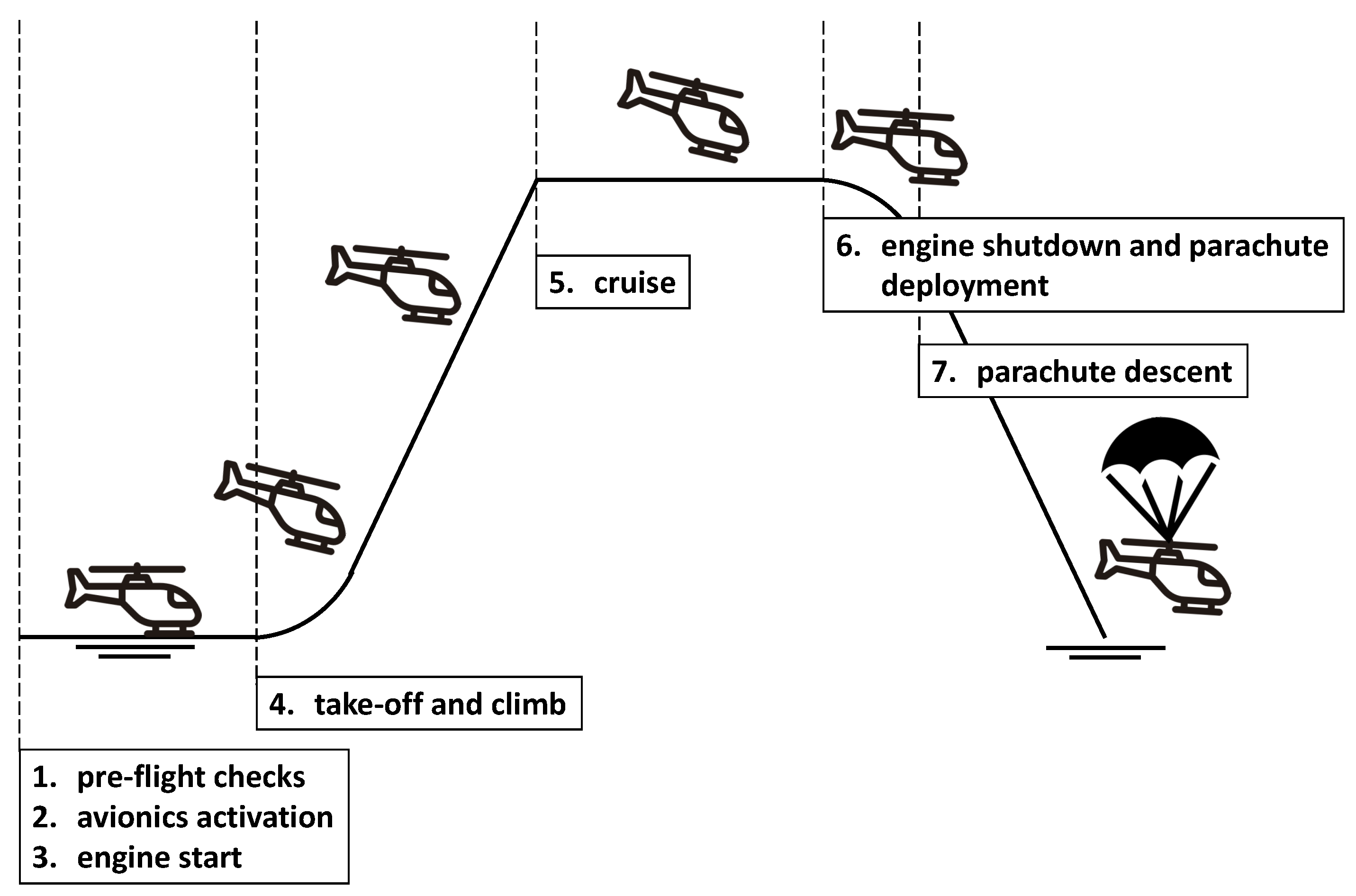
- Pre-flight checks: the systems involved in the mission are prepared and visually checked. The helicopter is placed on flat terrain at a safety distance from the GCS. The airfield is required to be clear of obstacles while the mission airspace is circumscribed by a radius of 5 km and a height of 500 m with respect to the GCS.
- Avionics power-on: both the ground and the flight segment subsystems are activated. Telemetry data are received by the GCS, and software/hardware verification checks are performed. The pilot validates the correct actuation of control commands.
- Engine start: the ignition procedure is started by the pilot’s action and the turbine reaches the idle condition.
- Take-off and climb: the helicopter takes-off and climbs out of ground effect at a controlled rate until reaching 300 m above the airfield.
- Cruise: the helicopter is stabilized in steady level flight at about 30 kts.
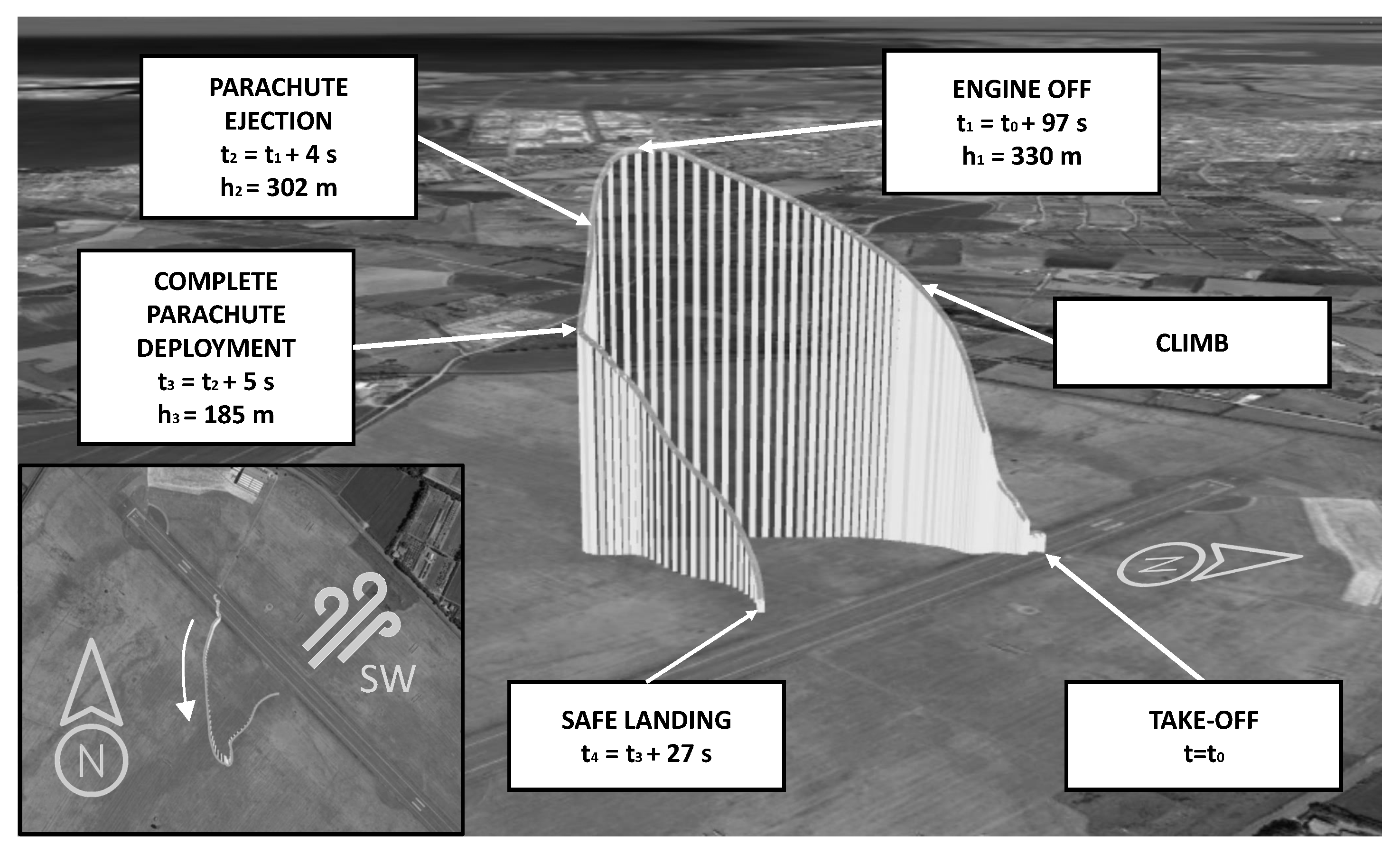
- Engine shutdown and parachute ejection: the pilot performs the termination procedure, which includes engine shutdown and parachute ejection.
- Descent: the helicopter descends with a stabilized speed and lands within the prescribed area.
2.2. System Architecture
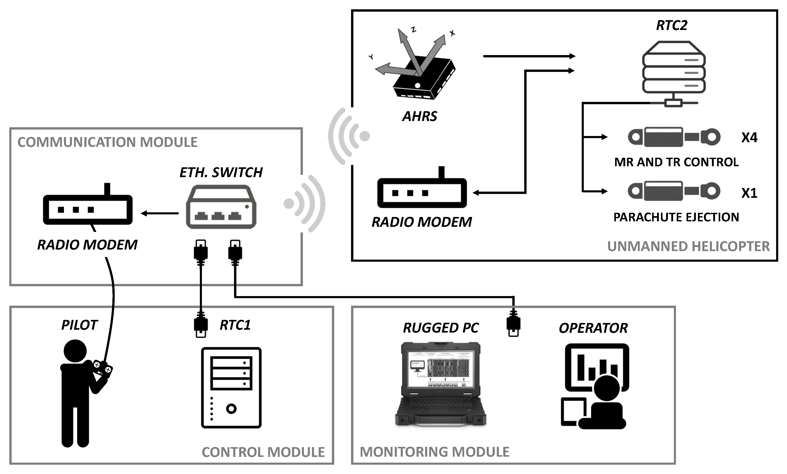
- the control module, where a modified commercial-off-the-shelf Radio Controller (RC) is used as a human-machine interface. Commands from the pilot, represented by stick deflections and switch activation inputs, are generated as Pulse-Width Modulated (PWM) signals and collected via the Pulse-Position Modulation (PPM) protocol. The PPM signal is finally provided to an integrated micro-controller board and output to the communication module according to serial protocol;
- the monitoring module, represented by a rugged laptop, where a graphical user interface is designed to display telemetry data, plan the mission, and send high-level commands via an Ethernet TCP/IP connection to a Real-Time Computer (RTC1) for data acquisition and processing;
- the communication module, which provides an RX/TX radio link to the flight segment. An ethernet switch is used to collect data from the monitoring module, while a ground-based radio modem is connected to a pair of 8 dBi GHz directional patch antennas (respectively characterized by right-hand circular and vertical polarization).
- a corresponding radio modem. Data are output via serial protocol and converted to a widespread standard industrial bus for communication with the Flight Management System (FMS);
- a Real-Time Computer (RTC2) performing FMS data acquisition and control tasks;
- a combined navigation and Attitude and Heading Reference System (AHRS) to estimate attitude information in a dynamic environment, along with position and velocity. Data are output via serial protocol and converted to a standard industrial bus for communication with the FMS;
- a set of 4 EMAs controls the collective, lateral, and longitudinal blade pitches of the MR and the collective pitch of the TR. An additional EMA is used for parachute deployment actuation. An FTS, based on a separate 868 MHz radio system, allows the Fuel Shut-Off Valve (FSOV) to close for emergency engine shutdown. The EMA and FTS selected for the experiment are devices available in the civil market.
3. System Modeling
3.1. Reference Frames
- an Earth-fixed North-East-Down frame, : the origin, , is arbitrarily fixed to a point on the Earth’s surface, aims in the direction of the geodetic North, points downwards along the Earth’s ellipsoid normal, and completes a right-handed triad. This frame is assumed to be inertial under the assumption of a flat and non-rotating Earth;
- a Local Vertical-Local Horizontal frame, : the origin is located at the vehicle’s center of gravity, . Under the hypothesis of a flat Earth, has axes parallel to ;
- a body-fixed frame, : the –axis is positive out the nose of the rotorcraft in its plane of symmetry, is perpendicular to in the same plane of symmetry, pointing downwards, and completes a right-handed triad;
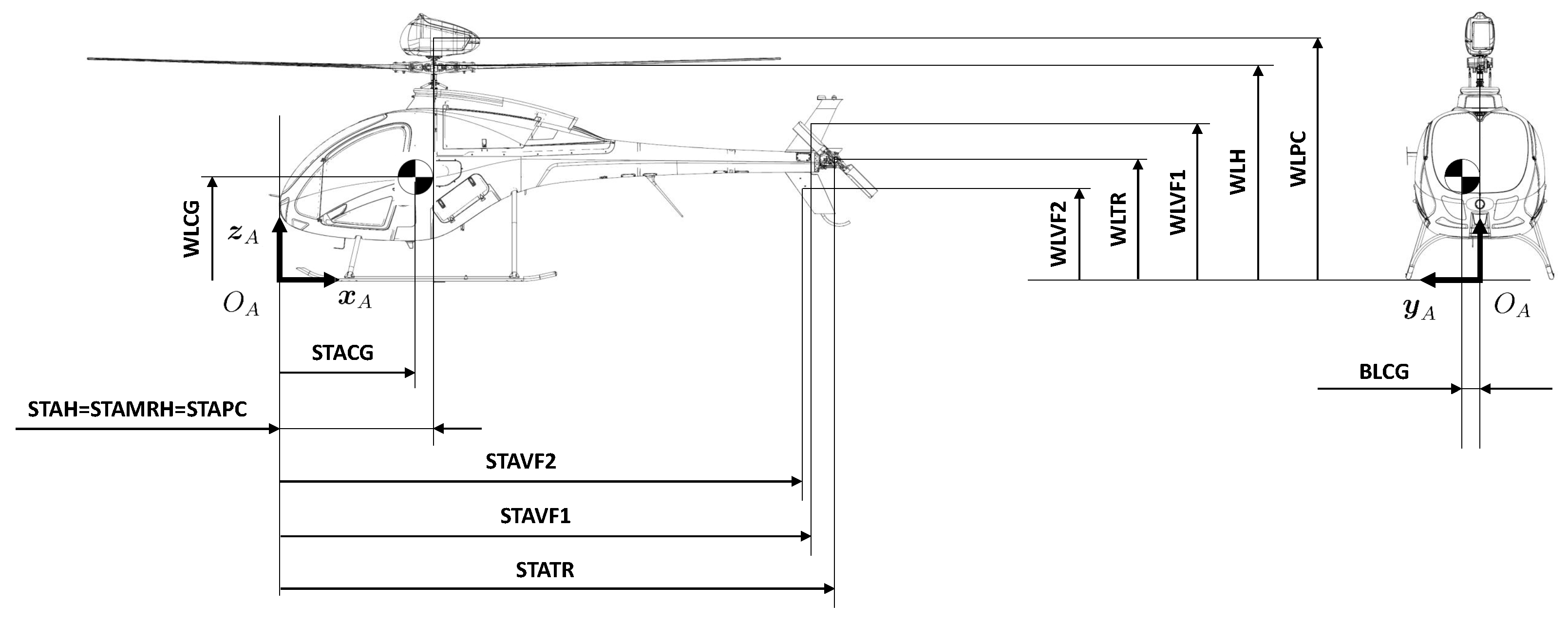
- an aircraft reference frame, , used to locate and all helicopter components: axes are parallel to the body-fixed frame axes, such that , , and . The origin is located ahead and below the rotorcraft at some arbitrary point within the plane of symmetry. Stations () are measured positive aft along the longitudinal axis. Buttlines () are lateral distances, positive to the pilot’s right, and waterlines () are measured vertically, positive upwards. A sketch of the rotorcraft, including the selected frame, is reported in Figure 4. The positions of the main components, expressed in , are listed in Table 1 and Table 2, together with relevant helicopter data.
3.2. Rigid Body Dynamics
3.3. Aerodynamic Forces and Moments
3.3.1. MR and TR Modeling
3.3.2. Fuselage, Empennages, and Miscellaneous Components
4. Trim and Stability Analysis
4.1. Trim Analysis
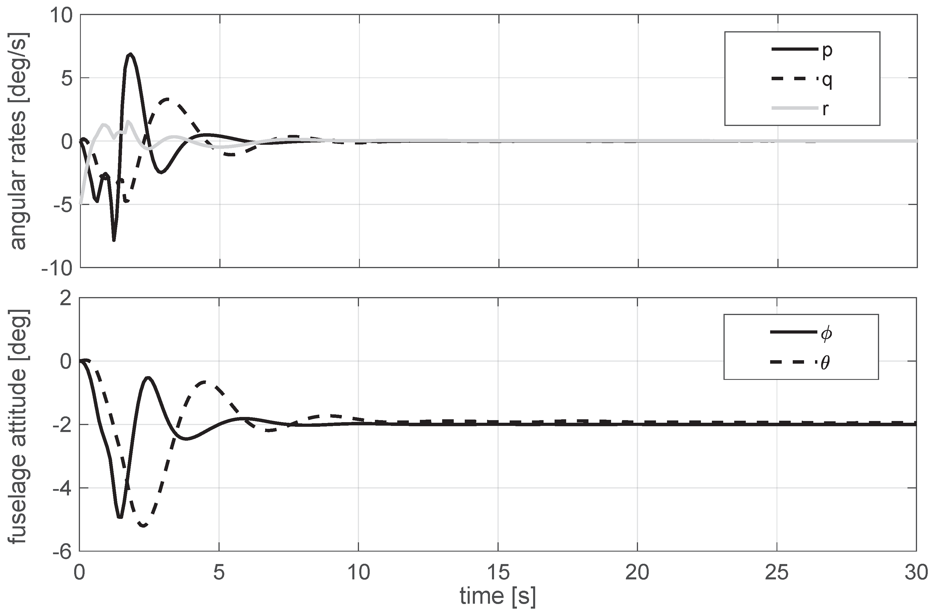
4.2. Dynamic Analysis
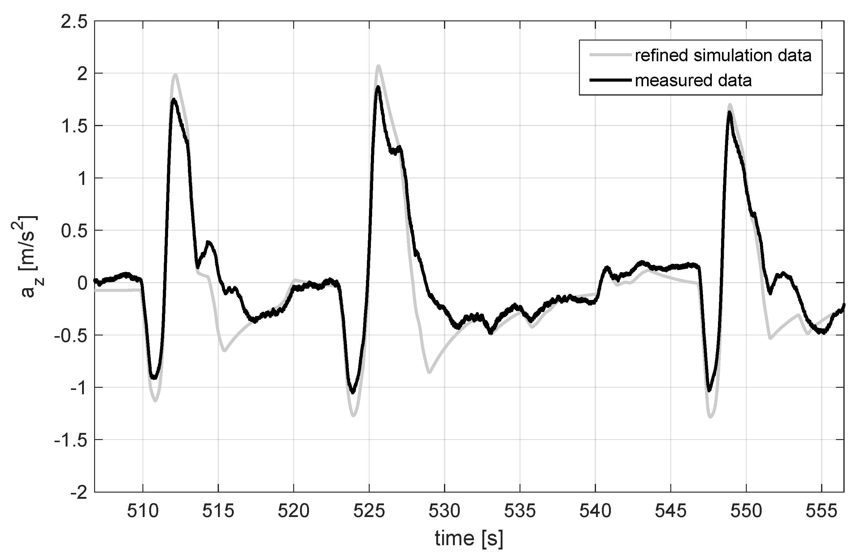
4.3. Model Validation
5. Control System Design and Test
5.1. Model–in–the–Loop Validation
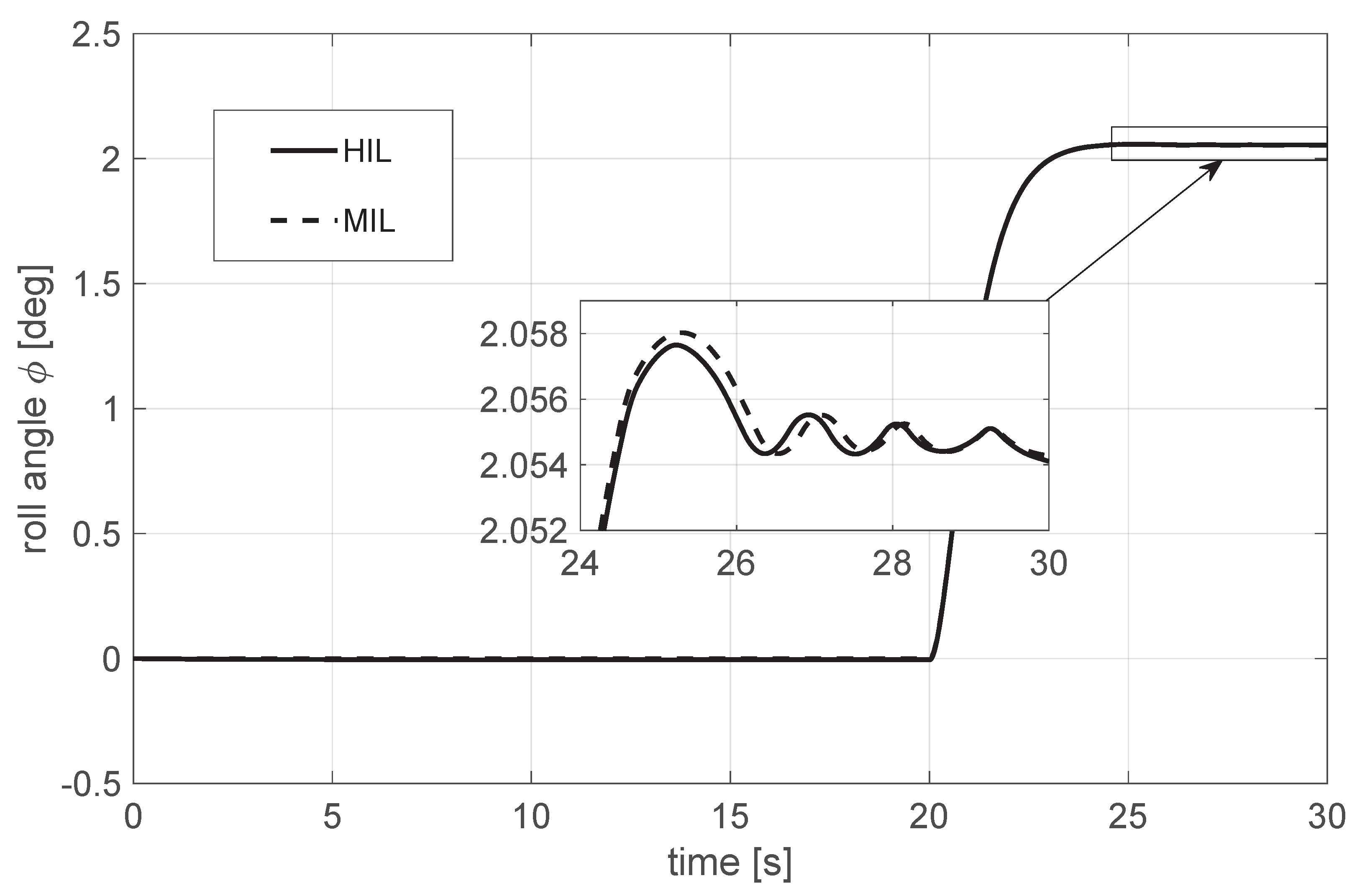
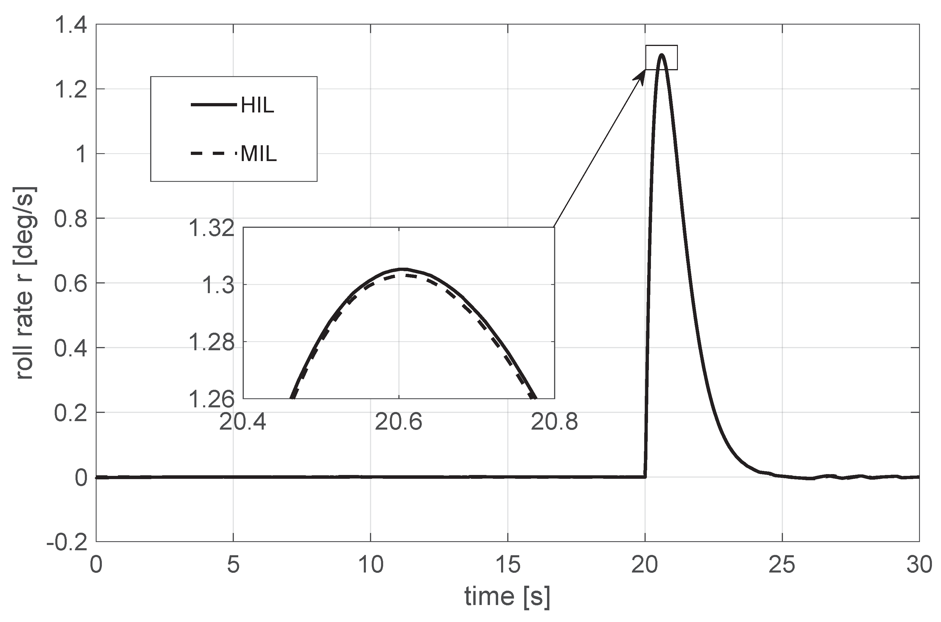
5.2. Hardware–in–the–Loop Validation
- The software developed in Matlab/Simulink for the mathematical modeling of helicopter dynamics and AHRS devices is automatically coded and deployed to a high-performance Real-Time Target Machine (RTTM) by Simulink Real-TimeTM tools. Solver frequency is set at 20 kHz, while AHRS model data are generated at 100 Hz. Software coding and deployment are performed through a host desktop PC, where the FlightGear open-source application is used to represent simulation data through a 3D graphical interface.
- The output of RTTM is provided via a dedicated standard industrial bus I/O module with two isolated ports. The first port is used to output the emulated AHRS data. The second port is used to generate repeatable control commands for HIL validation only, as if they were provided by the pilot on the ground.
- AHRS data and pilot commands from the RC device are the inputs to the onboard computer. At the time of the HIL experiments the RTC2, was already mounted on the helicopter as a pure acquisition device for an extensive campaign of manned flight tests. Hence, laboratory HIL tests were performed by arranging the RTC1 as an onboard computer. To emulate the presence of the radio modem, signals from the RC are converted from serial to standard industrial protocol by a micro-controller board equipped with a dedicated conversion shield. The control laws designed in Matlab/Simulink are coded and deployed to the RTC1 through the rugged laptop. The code developed for the onboard computer makes use of proprietary libraries for PID control implementation, acquisition and processing of input signals (including the application of Butterworth filters with order 1 and a cut-off frequency of 5 Hz to measured data), and real-time monitoring of selected variables.
- Control signals are acquired through a terminal board by a dedicated I/O module, a 16 bit analog input device selected to close the control loop. An ad hoc test bench is also provided where 1 EMA is controlled, in turn, by a voltage signal. Information about the linear motion are acquired and made available to evaluate the actuation performance.
6. Flight Tests with the Unmanned Helicopter
- Step 1. Direct control of onboard actuators by remote pilot commands, such that , , , and . This piloting configuration allows for validation of the overall actuation setup and represents a reversion mode in case of AHRS failure (manual mode).
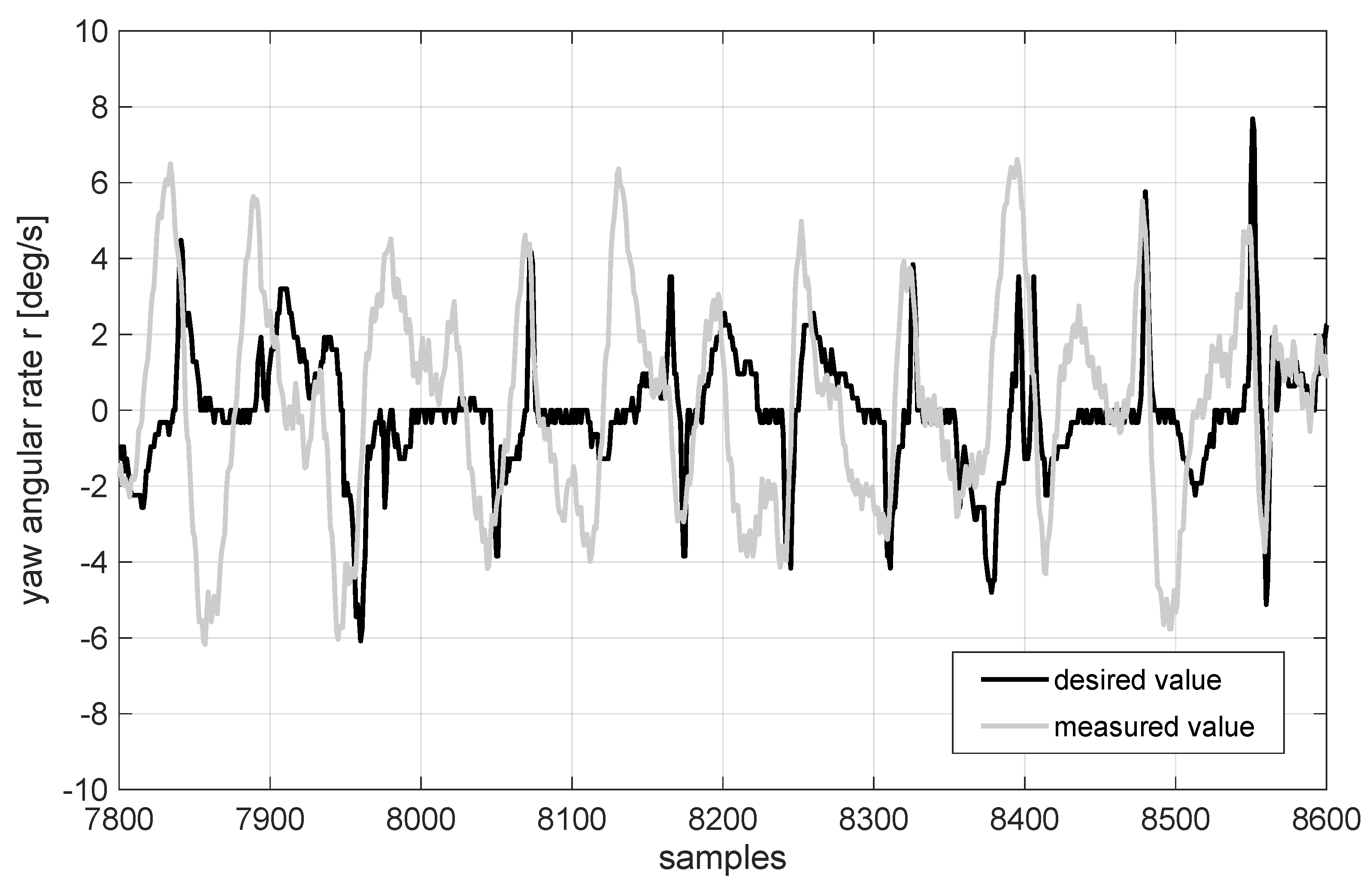
- Step 2. The controller in Equation (27) is activated in order to stabilize the yaw rate. Different flight tests are performed and control gains are refined according to remote pilot recommendations, such that and are respectively increased by about and with respect to the first-guess values in Section 5.1.
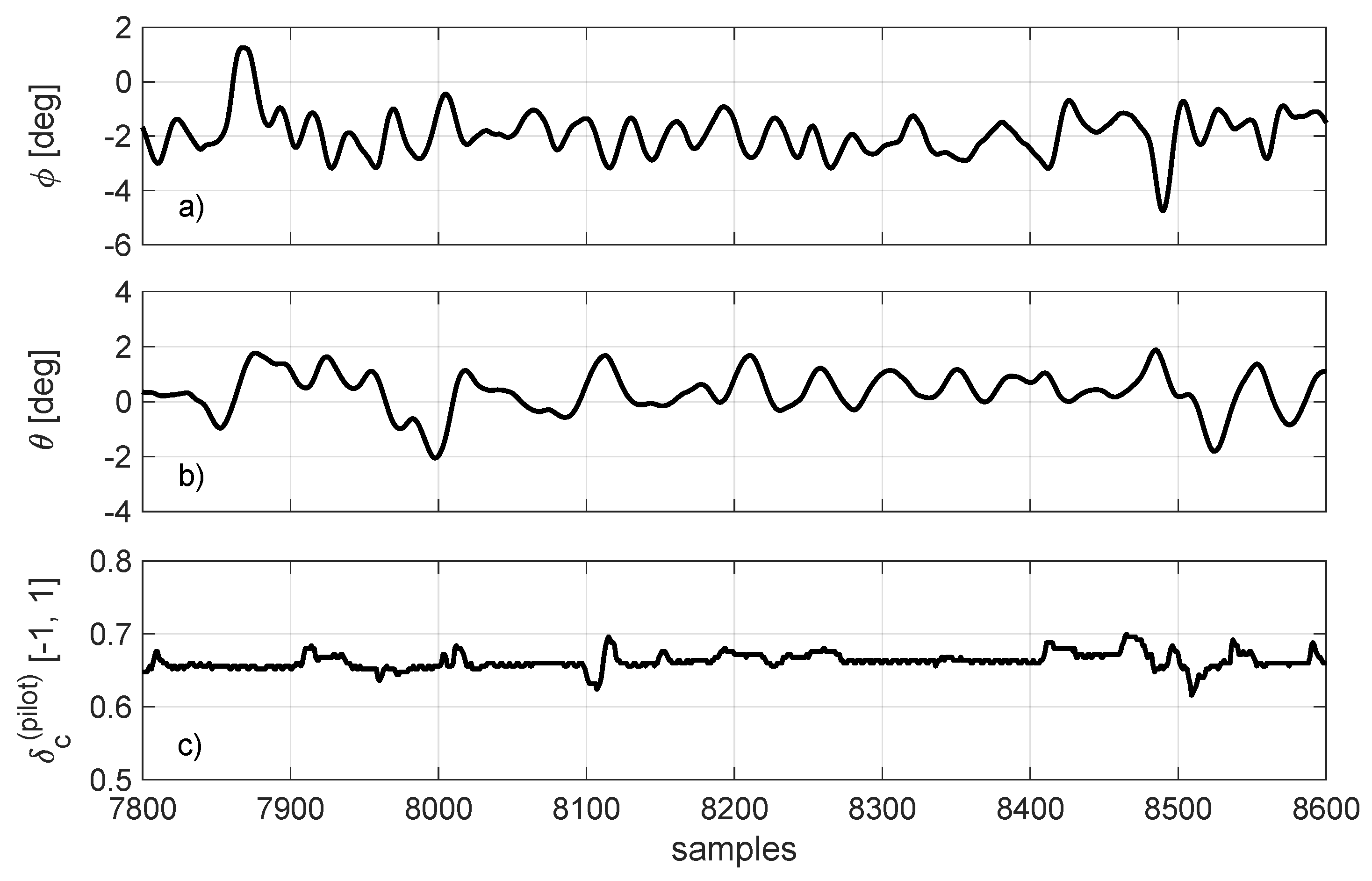
- Step 3. Before activating the controllers in Equations (28) and (29), an intermediate test is performed in order to evaluate the damping contribution only provided by gains and to the flying qualities about the roll and the pitch axis, respectively. To this end, the yaw rate is stabilized as in Step 2, while the direct control action of the pilot on lateral and longitudinal cyclic commands is supported by roll and pitch damper controllers, configured as follows:At the end of Step 3, control gains are fine-tuned such that and are respectively increased by about and with respect to the first-guess values.
- Step 4. The attitude controllers in Equations (28) and (29) are investigated, leaving the pilot with direct control of MR collective pitch only. Control gains are corrected such that and are respectively increased by and with respect to the precautionary small values proposed in Section 5.1. Finally, and are left unaltered.
7. Conclusions
Author Contributions
Funding
Data Availability Statement
Acknowledgments
Conflicts of Interest
References
- Garrow, L.A.; German, B.J.; Leonard, C.E. Urban air mobility: A comprehensive review and comparative analysis with autonomous and electric ground transportation for informing future research. Transp. Res. Part. C Emerg. Technol. 2021, 132, 1–31. [Google Scholar] [CrossRef]
- de Angelis, E.L.; Giulietti, F. Dynamic stability and control of rotorcraft for suspended load transportation: An analytical approach. In Proceedings of the 48th European Rotorcraft Forum, Winterthur, Switzerland, 6–8 September 2022; pp. 1–14. [Google Scholar]
- Schneider, D. The delivery drones are coming. IEEE Spectrum 2020, 57, 28–29. [Google Scholar] [CrossRef]
- de Angelis, E.L.; Giulietti, F.; Pipeleers, G. Swing angle estimation for multicopter slung load applications. Aerosp. Sci. Technol. 2019, 89, 264–274. [Google Scholar] [CrossRef]
- Causa, F.; Fasano, G. Multiple UAVs trajectory generation and waypoint assignment in urban environment based on DOP maps. Aerosp. Sci. Technol. 2021, 110, 1–15. [Google Scholar] [CrossRef]
- Dai, W.; Pang, B.; Low, K.H. Conflict-free four-dimensional path planning for urban air mobility considering airspace occupancy. Aerosp. Sci. Technol. 2021, 119, 1–17. [Google Scholar] [CrossRef]
- Schweiger, K.; Knabe, F.; Korn, B. An exemplary definition of a vertidrome’s airside concept of operations. Aerosp. Sci. Technol. 2022, 125, 107144. [Google Scholar] [CrossRef]
- Le Tallec, C.; Joulia, A.; Harel, M. A personal plane air transportation system-The PPlane Project. SAE Int. J. Aerosp. 2011, 4, 1281–1292. [Google Scholar] [CrossRef]
- Hlinka, J.; Trefilova, H. Identification of major safety issues for a futuristic personal plane concept. Aviation 2014, 18, 120–128. [Google Scholar] [CrossRef]
- Shihab, S.A.M.; Wei, P.; Ramirez, D.S.J.; Mesa-Arango, R.; Bloebaum, C. By Schedule or on Demand?—A Hybrid Operation Concept for Urban Air Mobility. In Proceedings of the AIAA Aviation 2019 Forum, Dallas, TX, USA, 17–21 June 2019; pp. 1–13. [Google Scholar] [CrossRef]
- Boelens, J.H. The Road-Map to Scalable Urban Air Mobility, Volocopter White Paper 2021; Chapter 4. Available online: https://www.volocopter.com/content/uploads/Volocopter-WhitePaper-2-0.pdf (accessed on 23 November 2021).
- de Angelis, E.L.; Giulietti, F.; Pipeleers, G.; Rossetti, G.; Van Parys, R. Optimal autonomous multirotor motion planning in an obstructed environment. Aerosp. Sci. Technol. 2019, 87, 379–388. [Google Scholar] [CrossRef]
- de Angelis, E.L.; Giulietti, F.; Avanzini, G. Optimal cruise performance of a conventional helicopter. Proc. Inst. Mech. Eng. Part G J. Aerosp. Eng. 2021, 263, 865–878. [Google Scholar] [CrossRef]
- Hardesty, M.; Guthrie, D.; Cerchie, D. Unmanned Little Bird Testing Approach. In Proceedings of the 2009 American Helicopter Society International Technical Specialists Meeting on Unmanned Rotorcraft Systems, Phoenix, AZ, USA, 20–22 January 2009; pp. 1–12. [Google Scholar]
- Downs, J.; Prentice, R.; Dalzell, S.; Besachio, A.; Ivler, C.M.; Tischler, M.B.; Mansur, M.H. Control System Development and Flight Test Experience with the MQ–8B Fire Scout Vertical Take-Off Unmanned Aerial Vehicle (VTUAV). In Proceedings of the American Helicopter Society 63rd Annual Forum, Virginia Beach, VA, USA, 1–3 May 2007; pp. 1–27. [Google Scholar]
- Mansur, M.H.; Tischler, M.B.; Bielefield, M.D.; Bacon, J.W.; Cheung, K.K.; Berrios, M.G.; Rothman, K.E. Full flight envelope inner–loop control law development for the unmanned K–MAX. In Proceedings of the American Helicopter Society 67th Annual Forum, Virginia Beach, VA, USA, 3–5 May 2011; pp. 1–17. [Google Scholar]
- Perry, D. Eurocopter Demonstrates Unmanned EC145. Flight Global. 2013. Available online: https://www.flightglobal.com/video-eurocopter-demonstrates-unmanned-ec145/109550.article (accessed on 23 November 2021).
- Adams, E. A Tap–to–Fly Helicopter Shows How Flying Cars Might Take Off. Wired. 2019. Available online: https://www.wired.com/story/sikorsky-sara-helicopter-autonomous-flying-car-air-taxi-tech/ (accessed on 23 November 2021).
- Curti Costruzioni Meccaniche, The New Zefhir Helicopter by Curti Aerospace Division. Available online: https://www.zefhir.eu (accessed on 23 November 2021).
- Bertolani, G.; Ryals, A.D.; Pollini, L.; Giulietti, F. L1 adaptive speed control of a helicopter. In Proceedings of the 48th European Rotorcraft Forum, Winterthur, Switzerland, 6–8 September 2022; pp. 1–11. [Google Scholar]
- Pavel, M.D.; Bertolani, G.; Giulietti, F. Non–linear (incremental) backstepping control applied to helicopter flight. In Proceedings of the 48th European Rotorcraft Forum, Winterthur, Switzerland, 6–8 September 2022; pp. 1–14. [Google Scholar]
- Huber, M. Zefhir Successfully Tests Whole Helicopter Parachute. AINonline. 2018. Available online: https://www.ainonline.com/aviation-news/general-aviation/2018-09-28/zefhir-successfully-tests-whole-helicopter-parachute (accessed on 23 November 2021).
- Head, E. How Curti Put a Parachute on Its Zefhir Helicopter. Vertical. 2019. Available online: https://verticalmag.com/news/curti-parachute-zefhir-helicopter/ (accessed on 23 November 2021).
- Abdelmaksoud, S.I.; Mailah, M.; Abdallah, A.M. Control Strategies and Novel Techniques for Autonomous Rotorcraft Unmanned Aerial Vehicles: A Review. IEEE Access 2020, 8, 195142–195169. [Google Scholar] [CrossRef]
- Talbot, P.D.; Tinling, B.E.; Decker, W.A.; Chen, R.T. A Mathematical Model of a Single Main Rotor Helicopter for Piloted Simulation; NASA TM 84281; NASA: Washington, DC, USA, 1982; pp. 1–55.
- Department of Defense. World Geodetic System 1984—Its Definition and Relationship with Local Geodetic Systems; DMA TR 8350.2; Department of Defense: Arlington, VA, USA, 1991; Chapter 5.
- U.S. Government Printing Office. U.S. Standard Atmosphere; NOAA-S/T 76-1562; U.S. Government Printing Office: Washington, DC, USA, 1976; Chapter 2.1.
- Leishman, J.G. Principles of Helicopter Aerodynamics, 2nd ed.; Cambridge University Press: New York, NY, USA, 2006; Chapters 2 and 5. [Google Scholar]
- Padfield, G.D. Helicopter Flight Dynamics, 2nd ed.; Blackwell Pub.: Oxford, UK, 2007; Chapter 3. [Google Scholar]
- Scavo, T.R.; Thoo, J.B. On the geometry of Halley’s method. Am. Math. Mon. 1995, 102, 417–426. [Google Scholar] [CrossRef]
- Jewel, J.W.; Heyson, H.H. Charts of the Induced Velocities Near a Lifting Rotor; NASA TM 4-15-59L; NASA: Washington, DC, USA, 1959; pp. 1–68.
- Dormand, J.R.; Prince, P.J. A family of embedded Runge-Kutta formulae. J. Comput. Appl. Math. 1980, 6, 19–26. [Google Scholar] [CrossRef]
- Tischler, M.B. Advances in Aircraft Flight Control, 1st ed.; Taylor & Francis: London, UK, 1996; Chapter 2. [Google Scholar] [CrossRef]
- Tischler, M.B.; Fletcher, J.W.; Diekmann, V.L.; Williams, R.A.; Cason, R.W. Demonstration of Frequency Sweep Testing Technique Using a Bell 214–ST Helicopter; NASA TM 89422; NASA: Washington, DC, USA, 1987; Chapters 5 and 6.
- Ljung, L. Prediction error estimation methods. Circuits Syst. Signal Process. 2002, 21, 11–21. [Google Scholar] [CrossRef]
- Cai, G. Design and implementation of a hardware–in–the–loop simulation system for small–scale UAV helicopters. In Proceedings of the 2008 IEEE International Conference on Automation and Logistics, Qingdao, China, 1–3 September 2008; pp. 29–34. [Google Scholar] [CrossRef]


| Parameter | Symbol | Computer Mnemonic | Value | Units |
|---|---|---|---|---|
| Main Rotor | ||||
| MR radius | ROTOR | 3.8 | m | |
| MR chord | CHORD | 0.195 | m | |
| MR rotational speed | OMEGA | 528.5 | rpm | |
| MR Lock number | GAMMA | 4.25 | - | |
| MR hinge offset | EPSLN | 0 | percent/100 | |
| MR flapping spring constant | AKBETA | 0 | N m/rad | |
| MR tangent of | AKONE | 0 | - | |
| MR solidity | SIGMA | 0.0327 | - | |
| MR hub stationline | STAH | 2 | m | |
| MR hub buttline | BLH | 0 | m | |
| MR hub waterline | WLH | 2.4 | m | |
| Tail Rotor | ||||
| TR radius | RTR | 0.57 | m | |
| TR chord | cTR | 0.12 | m | |
| TR rotational speed | OMTR | 3 061.8 | rpm | |
| TR tangent of | FKITR | 1 | - | |
| TR solidity | STR | 0.0382 | - | |
| MR hub stationline | STATR | 6.4 | m | |
| MR hub buttline | BLTR | −0.25 | m | |
| MR hub waterline | WLTR | 1.34 | m |
| Parameter | Symbol | Computer Mnemonic | Value | Units |
|---|---|---|---|---|
| Fuselage (Fus.) | ||||
| Fus. aerodynamic ref. point stationline | STARPF | 0 | m | |
| Fus. aerodynamic ref. point buttline | BLRPF | 0 | m | |
| Fus. aerodynamic ref. point waterline | STARPF | 0 | m | |
| Horizontal stabilizer (HS) | ||||
| HS stationline | STAHS | 6.199 | m | |
| HS buttline | BLHS | 0.435 | m | |
| HS waterline | WLHS | 1.394 | m | |
| Upper vertical fin (VF1) | ||||
| VF1 stationline | STAVF1 | 6.1 | m | |
| VF1 buttline | BLVF1 | 0.052 | m | |
| VF1 waterline | WLVF1 | 1.683 | m | |
| Lower vertical fin (VF2) | ||||
| VF2 stationline | STAVF2 | 6.069 | m | |
| VF2 buttline | BLVF2 | 0.048 | m | |
| VF2 waterline | WLVF2 | 0.996 | m | |
| Main rotor hub (MRH) | ||||
| MRH stationline | STAMRH | 2 | m | |
| MRH buttline | BLMRH | 0 | m | |
| MRH waterline | WLMRH | 2.4 | m | |
| Parachute canopy (PC) | ||||
| PC stationline | STAPC | 2 | m | |
| PC buttline | BLPC | 0 | m | |
| PC waterline | WLPC | 2.468 | m |
| Parameter | Symbol | Value | Units | Est. Error |
|---|---|---|---|---|
| Main Rotor | ||||
| Long. first–harmonic flapping coeff. | 2.92 | deg | N/A | |
| Lat. first–harmonic flapping coeff. | −1.10 | deg | N/A | |
| Induced speed | 7.79 | m/s | N/A | |
| Aerodynamic torque | Q | 1 579.5 | Nm | 3.1% |
| Tail Rotor | ||||
| Long. first–harmonic flapping coeff. | 0.24 | deg | N/A | |
| Lat. first–harmonic flapping coeff. | −0.24 | deg | N/A | |
| Induced speed | 11.64 | m/s | N/A | |
| Aerodynamic torque | 26.1 | Nm | 4.4% | |
| Fuselage | ||||
| Roll angle | −2 | deg | 17.6% | |
| Pitch angle | −1.96 | deg | 6.7% | |
| Control Pitch Angles | ||||
| MR lat. cyclic pitch | −1.10 | deg | 4.8% | |
| MR lon. cyclic pitch | −2.91 | deg | 42.0% | |
| MR collective pitch | 12.62 | deg | 2.1% | |
| TR collective pitch | 8.28 | deg | 2.1% |
Disclaimer/Publisher’s Note: The statements, opinions and data contained in all publications are solely those of the individual author(s) and contributor(s) and not of MDPI and/or the editor(s). MDPI and/or the editor(s) disclaim responsibility for any injury to people or property resulting from any ideas, methods, instructions or products referred to in the content. |
© 2023 by the authors. Licensee MDPI, Basel, Switzerland. This article is an open access article distributed under the terms and conditions of the Creative Commons Attribution (CC BY) license (https://creativecommons.org/licenses/by/4.0/).
Share and Cite
de Angelis, E.L.; Giulietti, F.; Rossetti, G.; Turci, M.; Albertazzi, C. Toward Smart Air Mobility: Control System Design and Experimental Validation for an Unmanned Light Helicopter. Drones 2023, 7, 288. https://doi.org/10.3390/drones7050288
de Angelis EL, Giulietti F, Rossetti G, Turci M, Albertazzi C. Toward Smart Air Mobility: Control System Design and Experimental Validation for an Unmanned Light Helicopter. Drones. 2023; 7(5):288. https://doi.org/10.3390/drones7050288
Chicago/Turabian Stylede Angelis, Emanuele Luigi, Fabrizio Giulietti, Gianluca Rossetti, Matteo Turci, and Chiara Albertazzi. 2023. "Toward Smart Air Mobility: Control System Design and Experimental Validation for an Unmanned Light Helicopter" Drones 7, no. 5: 288. https://doi.org/10.3390/drones7050288