Chattering Reduction of Sliding Mode Control for Quadrotor UAVs Based on Reinforcement Learning

Abstract

Sliding mode control, an algorithm known for its stability and robustness, has been widely used in designing robot controllers. Such controllers inevitably exhibit chattering; numerous methods have been proposed to deal with this problem in the past decade. However, in most scenarios, ensuring that the specified form and the parameters selected are optimal for the system is challenging. In this work, the reinforcement-learning method is adopted to explore the optimal nonlinear function to reduce chattering. Based on a conventional reference model for sliding mode control, the network output directly participates in the controller calculation without any restrictions. Additionally, a two-step verification method is proposed, including simulation under input delay and external disturbance and actual experiments using a quadrotor. Two types of classic chattering reduction methods are implemented on the same basic controller for comparison. The experiment results indicate that the proposed method could effectively reduce chattering and exhibit better tracking performance.

1. Introduction

Unmanned aerial vehicles (UAVs) have been widely integrated into industrial production and civil use, such as aerial photography, plant protection, and military operations, owing to their simple structure and high mobility. However, UAVs represent a highly intricate system characterized by complicated coupling and nonlinear behaviors. Additionally, environmental factors such as wind, air pressure, and temperature changes can further introduce interference. Over the past decades, numerous methods have been proposed to address these challenges.

Nonlinearity and unknown external disturbances are inherent in UAV systems. To enhance the robustness of proportional–integral–derivative control (PID) [1], several robust methods, such as intelligent control [2,3,4], fuzzy control [5,6,7], model predictive control [8], and sliding mode control (SMC) [9,10,11,12,13], have been proposed. Among them, SMC is a model-based method with strong robustness to external disturbances and uncertainties, including equivalent control for realizing target tracking and switching control for suppressing nonlinear parts. The switching control can drive the system state to slide on the sliding surface according to the state error, and the nonlinear part can be shown as a linear behavior near the sliding surface, hence realizing the suppression and control of the nonlinear part [14].

Thus, this algorithm is effective for nonlinear systems and can fit well with UAVs. However, unmodeled higher-order dynamics and input delays are not conducive to the nonlinear output from tiny switching. They render it difficult to keep the state entirely at the sliding surface and are manifested as state transfer between the two sides of the sliding surface; this phenomenon is called chattering [15].

The chattering frequency is related to the controller, and the high-frequency switching output will harm the system. Over the years, numerous solutions have been proposed to deal with this problem.

Matouk et al. proposed a super twist algorithm based on a second-order SMC to design the UAV’s position and attitude controller [16]. Jayakrishnan et al. [17] used a cascaded inner and outer structure and a super-torsional SMC to design a quadrotor controller and demonstrated its superiority by comparing it with the linear quadratic regulator PD method. Adaptive methods are often used to deal with chattering. Lei and Li [18] used the sigmoid function to design an adaptive gain-tuning law that can effectively relax restrictions on prior information about system uncertainty. Yang and Yan [19] proposed a fuzzy system based on Gaussian membership functions to adaptively tune the switching gain in the attitude controller. Additionally, disturbance observers are widely used in controller design [20]. To deal with the external disturbances, Zhang et al. proposed a chattering-free discrete SMC based on disturbance observers [21]. Xu et al. combined an extended state observer and fast terminal SMC, thereby proposing a composite method to improve tracking performance while reducing chattering [22]. Subsequently, the symbolic function was replaced with a smoothing function to resolve chattering [23]. Le and Kang proposed a terminal SMC to guarantee that the tracking error converged to zero in finite time [24]. However, this method is limited by a low convergence rate and singularity. Consequently, fast TSMC [25], nonsingular TSMC [26], and nonsingular fast TSMC [27] were proposed to overcome these problems.

Nonetheless, these approaches commonly encounter a challenge: identifying the optimal mechanism for a specific system. For instance, in various methods, challenges arise in designing adaptive rules, determining the symbolic function strategy, and choosing optimal parameters for each mechanism. Consequently, intelligent learning methods were considered to explore the optimal mechanisms applicable to the system. By employing intelligent learning methods, these studies aim to overcome the aforementioned challenges and identify the most suitable agents for the determined system.

Reinforcement learning (RL) is a mechanism that learns to map states to actions for maximum rewards. It has been widely used in many fields [28,29,30]. As the potential of learning algorithms is explored, some learning-based methods have been proposed to solve the chattering in SMC. Farjadian et al. [31] introduced an adaptive gradient saturation function to replace the discontinuous switching function and used RL to adjust the slope to trade off control accuracy for a decrease in chattering. Their study is based on the saturation function and uses RL to realize adaptive control; however, the selected saturation function limits the final effect. Another study [32] proposed a method to solve the optimal control under constraints by applying the hyperbolic tangent and symmetry radial basis functions to design the saturating function. Subsequently, integral Q-learning was used to approximate it to reduce chattering. However, the Q-learning algorithm relies on the Q table, which limits the state’s dimension and makes the algorithm unsuitable for complex systems. Existing intelligent chattering reduction methods always accompany custom functions. This results in the network being limited by the selected function, which restricts the advantage of reinforcement learning.

Based on the above discussion, to avoid the problems of state dimension limitation [32] and auxiliary function limitation [31] in the existing works, this study combines a policy-based RL method to solve the chattering problem in SMC. Specifically, a reference model-based SMC was adopted as the base controller. In the nonlinear part, the reward function is designed based on the state tracking error, and the network output that produces the maximum reward is directly involved in the controller as the switching control. Notably, no additional functions are employed to restrict the network output. The contributions of this study can be summarized as follows:

• A method using RL to reduce chattering in SMC was proposed. The reference model-based SMC was designed and implemented based on the easy-obtained fitted model.
• The policy-based DDPG algorithm was employed to explore optimal switching control and produce continuous nonlinear outputs. In contrast to [31], no auxiliary function was utilized; the actions generated by the network were regarded as switching outputs and contributed to the final control output.
• Two classical methods were selected to improve the same basic SMC and compared with the proposed method. Experiment results revealed that the proposed method can solve chattering well and better tolerate the delay and disturbance of the system compared to the two classical methods.

The remainder of this paper is organized as follows: Section 2 analyzes the dynamics of the UAV system. Section 3 describes the proposed RL-based controller design process in detail. Section 4 demonstrates the validation of the proposed algorithm. Finally, the conclusions are summarized in Section 5.

2. Chattering Problem and Attitude Dynamics

2.1. Chattering in Sliding Mode Control

In UAV systems, external disturbances inevitably exist, and the controller output is also relatively delayed owing to the system’s inertia, making the chatter more likely. Subsequently, chattering causes vibrations in the UAV and leads to the heating of the rotor, which increases energy consumption and reduces the service life of the power system.

According to the studies mentioned in Section 1, the classic methods to reduce chattering can be mainly classified into the following categories:

Class A: These methods design a time-varying switching gain, whereby the controller’s sensitivity to external disturbances is reduced by changing the switching gain, consequently reducing chattering, such as in [18,19].

Class B: These methods replace the symbolic functions with the self-defined functions and use switch control outside the boundary layer, whereas linear feedback control is used inside, such as in [23,24,25,26,27].

Class C: These methods estimate the disturbance and compensate for it, such as in [21,22].

Methods in Class A need to formulate suitable adaptive laws, whereas Class B needs to select the appropriate nonlinear function, and Class C must design reasonable observers for the system. In different method design processes, the mechanism and the parameters used are influenced by the subjective factors of the researchers. Thus, verifying whether the proposed method is optimal for the specific system is challenging.

2.2. Attitude Dynamics

Owing to the underactuated characteristics of the classic quadrotor, the control system is generally developed based on the cascade structure. Taking the horizontal direction as an example, the control system can be divided into position control, attitude control, and stability control. The attitude control is based on attitude feedback and is crucial to maintaining the balance of the UAV. The accuracy and stability of the controller can significantly affect the performance of the UAV in practical applications.

Newton–Euler equations usually express UAV models; however, accurate parameters are generally difficult to obtain. Therefore, ignoring the coupling effect and sacrificing the model’s accuracy, a simple and easy-to-obtain approximate model based on fitting data is an excellent alternative. Considering attitude dynamics, the controller’s output ${\omega }_r$ is the input of the inner stabilize controller. Considering the attitude system with input ${\omega }_r$ and output $\mu$, a second-order transfer function (1) can well characterize the behavior of the system  [23,33,34].

$$G\left(s\right)=\frac{b_0}{s^2+a_{0}s+a_1}$$

(1)

where $a_0$, $a_1$, and $b_0$ can be obtained according to the pre-collected flight data of the UAV. The pre-collected data can be obtained and recorded by operating the actual UAV under stabilize control; ${\omega }_r$ was given directly from the remote control during the collection process. According to the fitted model, the target attitude rate and the feedback satisfy.

$$\ddot{\omega }=-a_0\dot{\omega }-a_1\omega +b_0{\omega }_r.$$

(2)

According to [35], the motion in each axis can be neglected if the changes in UAV amplitude are less than 0.45 rad. Assume that the UAV satisfies the following conditions: the altitude does not change when the UAV moves in the horizontal direction; the heading always remains unchanged. Then, the attitude variables $\mu$ and $\omega$ can be approximated as $\dot{\mu }=\omega$.

Considering $X={[\dot{\omega },\omega ,\mu ]}^T$, and $\mu$ as the output, (2) can be rewritten as follows:

$$\left\{\begin{array}{c}\dot{X}=AX+Bu,\\ Y=CX.\end{array}\right.$$

(3)

The specific forms of A, B, and C in (3) are as follows:

$$\begin{array}{c}A=\left[\begin{array}{ccc}-a_0& -a_1& 0\\ 1& 0& 0\\ 0& 1& 0\end{array}\right],B=\left[\begin{array}{c}{b}_0\\ 0\\ 0\end{array}\right],C=\left[\begin{array}{ccc}0& 0& 1\end{array}\right]\hfill \end{array}$$

(4)

3. Controller Design

3.1. System Overview

In this study, a reference model sliding mode controller was adopted as the basic controller; its outstanding performance was verified in our previous work [34]. The proposed method consists of a reference model, Kalman filter, neural network, and sliding mode controller; its structure is shown in Figure 1.

The reference model can expand the set of target states beyond the given original target, such as the target of attitude rate and acceleration. The attitude model used herein is based on the fitted system; thus, the attitude acceleration is considered in the controller. However, as directly measuring the attitude acceleration is difficult, a steady Kalman filter was adopted herein to estimate the difficult-to-measure state. Finally, the reference signal and the estimate feedback states were used to calculate the equivalent control $u_{eq}$, combined with the $u_{sw}$ output of the neural network; thus, the target could be well-tracked without chattering.

The significant advantage of this structure is that it separates the tracking and regulation stages. The time domain evaluation indicators, such as the rise time and settling time, and the general indicators, such as stability and tracking performance, can be designed individually by the reference model and the controller.

3.2. Reference Model

The reference model is closely related to the UAV model. According to the attitude model expressed in (3), the reference model can be designed as follows:

$$\left\{\begin{array}{c}{\dot{X}}_m=A_m{X}_m+B_m{r}_m,\hfill \\ Y_m=C_m{X}_m.\hfill \end{array}\right.$$

(5)

$r_m$ is the original attitude target, $X_m={[{\dot{\omega }}_m,{\omega }_m,{\mu }_m]}^T$ is the reference of each state, and its structure is similar to X, and the output matrix $C_m=C$. Similar to (4), the structure of $A_m$ in the reference model can be expressed as follows:

$$A_m=\left[\begin{array}{ccc}{a}_{m0}& a_{m1}& a_{m2}\\ 1& 0& 0\\ 0& 1& 0\end{array}\right],$$

(6)

where $a_{m0}$, $a_{m1}$, and $a_{m2}$ are negative constants that are tuned to realize the desired target trajectory. It is assumed that the designed reference model converges to the target within a finite time and that the state of the reference model remains constant after convergence. Moreover, the output of (5) equals the input. Then,

$$\left\{\begin{array}{c}{\dot{X}}_m=A_m{X}_m+B_m{r}_m=0,\hfill \\ Y_m=C_m{X}_m=r_m.\hfill \end{array}\right.$$

(7)

Assume that $A_m$ and $B_m$ satisfy the conditions expressed in (8) and (9),

$$B_m=B{K}_1,$$

(8)

$$A_m-A=B{K}_2.$$

(9)

When (8) is combined with (7), $K_1$ can be expressed as follows:

$$K_1={(-C_m{A}_m^{-1}B)}^{-1}.$$

(10)

Then, the input matrix $B_m$ in the reference model can be calculated by

$$B_m=B{(-C_m{A}_m^{-1}B)}^{-1}.$$

(11)

3.3. RL-Based Controller Design

The output of the neural network is directly utilized as a nonlinear control part to contribute to the total control output. Hence, the base controller should be introduced.

If the tracking error of the feedback and reference states is denoted as $E=X-X_m$, then the switching function can be designed.

$$\sigma =S_{c}E.$$

(12)

The selection parameter $S_c$ is a three-dimensional column vector corresponding to each state error. By combining the time derivative of the switching function, $\dot{\sigma }=S_c\dot{E}$, with Equations (3) and (5), and subject to the conditions (8) and (9), the resulting expression is

$$\begin{array}{c}\dot{\sigma }=S_c\dot{E},\\ =S_c(-B{K}_{2}X+A_{m}E+Bu-B{K}_{1}r).\end{array}$$

(13)

When the condition of the sliding mode is satisfied, the system states switch near the sliding surface; once the sliding surface is reached, the states remain on it and satisfy $\sigma =\dot{\sigma }=0$. The equivalent control, denoted by $u_{eq}$, can be calculated as follows:

$$u_{eq}=-{\left(S_{c}B\right)}^{-1}{S}_c{A}_{m}E+K_{2}X+K_{1}r.$$

(14)

Herein, the optimum theory was used to calculate $S_c$. The optimal feedback gain was chosen as the hyperplane $S_c=B^{T}P$, which satisfied the condition $S_{c}B>0$. The matrix P could be calculated using the Riccati equation, while Q is a designed positive diagonal matrix.

$$PA+A^{T}P-PB{B}^{T}P+Q=0.$$

(15)

Switching control (16) was introduced to suppress the nonlinear parts in the system, such as model error, interference, and uncertainty.

$$u_{sw}=K_{sw}f\left(\sigma \right),$$

(16)

where $K_{sw}=-c{\left(S_{c}B\right)}^{-1}$ is the gain coefficient, $c>0$ is the adjustable gain related to the unknown disturbance and model error, and $f\left(\sigma \right)=sign\left(\sigma \right)$ is typically adopted in the conventional scheme.

By combining (14) and (16), the result of reference model-based SMC can be obtained as follows:

$$u=u_{eq}+u_{sw}.$$

(17)

To reduce chattering in a specific system, the selection of $f\left(\sigma \right)$ always depends on the researchers’ experience. In this work, the RL method was combined with powerful exploration abilities to obtain the optimal output. Note that the output of the neural network is denoted as $\mathsf{\Phi }\left(\sigma \right)$, and the RL-improved nonlinear control $u_{sw}$ is

$$u_{sw}=K_{sw}\mathsf{\Phi }\left(\sigma \right).$$

(18)

By combining (14) and (18), the proposed RL-based sliding mode controller with improved chattering reduction can be expressed as follows:

$$u=-{\left(S_{c}B\right)}^{-1}{S}_c{A}_{m}E+K_{2}X+K_{1}r+K_{sw}\mathsf{\Phi }\left(\sigma \right).$$

(19)

The method of obtaining $\mathsf{\Phi }\left(\sigma \right)$ for the nonlinear control $u_{sw}$ is described in detail, as follows:

3.4. Nonlinear Output by RL

RL algorithms are often described in the context of the Markov decision process (MDP), which can be represented by a quadruple $(S,A,P,R,\gamma )$, the elements of which are a set of states, actions in the corresponding state, transition probability between states, reward after state transition, and decay factor, respectively.

Under policy $\pi$ and state s, the cumulative discounted return obtained during the period of taking a series of actions to reach the terminal state is called the value function $V^{\pi }\left(s\right)=E\left(R_t\right|S_t=s)$, and $E(\ast )$ reflects the expectation. According to $\pi$, starting from s and performing a, the expected return of all possible decision sequences is recorded as an action-value function $Q^{\pi }(s,a)=E\left(R_t\right|S_t=s,A_t=a)$. Each $\pi$ corresponds to a value function and state value function, whereas the optimal strategy ${\pi }^{*}$ corresponds to the optimal value function $V^{*}\left(s\right)$ and the optimal state-action value function $Q^{*}(s,a)$. Let ${\ast }^{\prime }$ be the next moment of ∗, then the Bellman equation can be expressed as follows:

$$\begin{array}{c}{V}^{*}\left(s\right)=maxE[r\left(s\right)+\gamma V^{*}\left(s^{\prime }\right)]\hfill \\ Q^{*}(s,a)=E[r(s,a)+\gamma \underset{a^{\prime }}{max}{Q}^{*}(s^{\prime },a^{\prime })].\hfill \end{array}$$

(20)

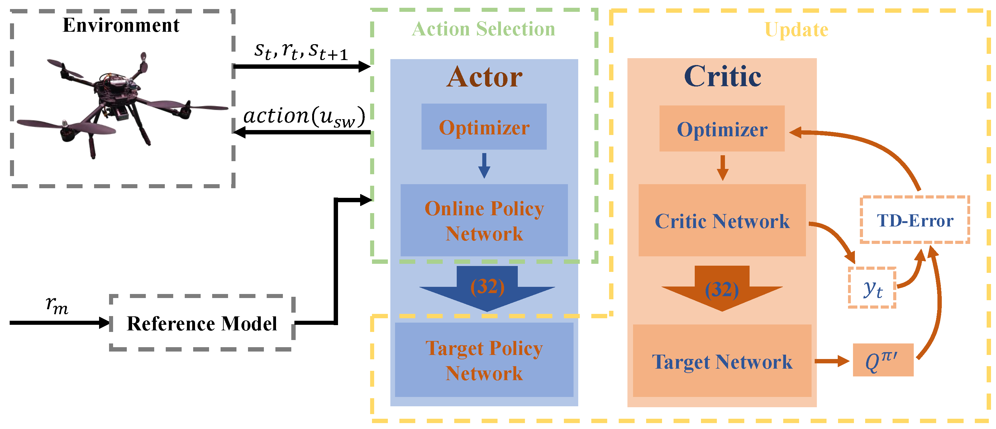
As the research object, the UAV system is characterized as complex and continuously time-varying, and the output of each controller must be deterministic and unique during the operation. Under such severe conditions, the deep deterministic policy gradient (DDPG) [36] algorithm, which performs well in continuous systems, is typically used. Based on actor-critic architecture, an RL scheme that includes an actor-network, an actor-target network, a critic-network, and a critic-target network was designed herein. A simplified training structure diagram is shown in Figure 2.

Combined with the reference state, the reward corresponding to the current action can be calculated according to the designed reward function (21). The aim of this study was to track the state of the target as quickly as possible and reduce chattering. Therefore, in the process of designing the reward, in addition to the attitude, the attitude rate, which is more sensitive to changes, deserves more of our attention. Among them, $Ref\left(s_k\right)$ represents the target value of the state, which is $Y_m$ in Section 3.2; $s_k$ means Y, and ${\lambda }_k>0$ is the weight represented by each state.

$$r_i=-\sum _{k=1}^n{\lambda }_k\left|Ref\left(s_k\right)-s_k\right|$$

(21)

In the DDPG, the network update is based on the difference between predicted and actual values. Under the deterministic strategy ${\pi }^{\prime }$, the Bellman equation can be rewritten as follows:

$$\begin{array}{c}\begin{array}{c}{Q}^{{\pi }^{\prime }}(s_t,a_t)=E_{{\pi }^{\prime }}[R(s_t,a_t)+\gamma E_{a_{t+1\sim {\pi }^{\prime }}}\left[Q^{{\pi }^{\prime }}(s_{t+1},a_{t+1})\right]].\hfill \end{array}\end{array}$$

(22)

To facilitate the distinction, ${\theta }^Q$ and ${\theta }^{\mu }$ are used to represent the parameters of the critic and actor-networks, respectively. Regarding the critic, the update of the neural network parameter adopts the temporal difference (TD)-error method, which is realized by the mean square error. Its loss function is defined as follows:

$$L\left({\theta }^Q\right)=\frac{1}{N}\sum _{t=1}^N{(Q(s_t,a_t|{\theta }^Q)-y_t)}^2,$$

(23)

where $y_t$ represents the output of the critic-target network with action reward, calculated as expressed in (24).

$$y_t=r(s_t,a_t)+\gamma Q(s_{t+1},\mu \left(s_{t+1}\right){\theta }^Q)$$

(24)

Thus, the gradient descent method is used to solve the gradient of the loss function in (23); subsequently, the critic-network parameters are updated according to the calculation results, as shown in (26), where $a_{{\theta }^Q}$ is the critic-network learning rate.

$$\begin{array}{c}{\nabla }_{{\theta }^Q}L\left({\theta }^Q\right)=\frac{1}{N}{\displaystyle \sum _{t=1}^N}[(y_t-Q(s_t,a_t|{\theta }^Q))\ast {\nabla }_{{\theta }^Q}Q(s_t,a_t|{\theta }^Q)],\end{array}$$

(25)

$$\begin{array}{c}{{\theta }^Q}_{t+1}={{\theta }^Q}_t+a_{{\theta }^Q}{\nabla }_{{\theta }^Q}L\left({\theta }^Q\right).\end{array}$$

(26)

Similarly, the actor-network is updated as shown in (27) and (28), where $a_{{\theta }^{\mu }}$ is the update rate of the actor-network.

$$\begin{array}{c}{\nabla }_{{\theta }^{\mu }}J\left({\theta }^{\mu }\right)=\frac{1}{N}{\displaystyle \sum _{t=1}^N}[{\nabla }_{{\theta }^{\mu }}\mu \left(s_t\right|{\theta }^{\mu })\ast {\nabla }_{a}Q(s_t,a_t|{\theta }^Q){|}_{a_t=\mu \left(s_t\right)}]\end{array}$$

(27)

$$\begin{array}{c}{{\theta }^{\mu }}_{t+1}={{\theta }^{\mu }}_t+a_{{\theta }^{\mu }}{\nabla }_{{\theta }^{\mu }}J\left({\theta }^{\mu }\right)\end{array}$$

(28)

Selecting the appropriate soft update rate $\tau$, the actor- and critic-target networks can be soft-updated by their respective non-target networks in the manner shown in (29).

$$\left\{\begin{array}{c}{\theta }^{Q^{\prime }}\leftarrow \tau {\theta }^Q+(1-\tau ){\theta }^{Q^{\prime }}\hfill \\ {\theta }^{{\mu }^{\prime }}\leftarrow \tau {\theta }^{\mu }+(1-\tau ){\theta }^{{\mu }^{\prime }}\hfill \end{array}\right.$$

(29)

The pseudocode of the entire reinforcement learning training process is presented in Algorithm 1.

Algorithm 1 Training process of the RL-based reference model SMC

Initialize the four network weights and replay buffer Load the UAV model and the reference model     while episode < MaxEpisode do    Initialize noise process    Initialize UAV states    Initialize reference model states        while timestep < MaxTimeStep do      Calculate the reference states $X_m$      Select action $a_t={\pi }^{\mu }\left(s_t\right)+n_t$      Calculate $u_s{}_w$, $u_e{}_q$ and run the model      Obtain $r_t$ and $s_{t+1}$      Save quadruple to D      Sample quadruple from D randomly      Critic-network updated using (25) and (26)      Actor-network updated using (27) and (28)      Target network updated using (29)      if $s_{t+1}$ not safe then         Break      end if    end while end while

4. Simulation and Experiment

The chattering reduction effect of the proposed RL-based SMC was verified by simulation and actual flight experiments.

4.1. Experimental Verification Platform

The experimental platform for the proposed algorithm application was a positive X-type quadrotor UAV with a 0.5 m wheelbase, and a self-developed flight control system based on the STM32F4 was adopted. The overall system, shown in Figure 3, consisted of a main control module, an inertial measurement unit (IMU) module, a global navigation satellite system (GNSS) module, and a data logging module.

The power system was composed of four 900 KV U2810 rotors and 11-inch propellers.

By collecting the attitude, attitude rate, and target attitude rate during flight, an approximate model can be fitted. The fitted model of the attitude model is $a_0=-49.5940$, $a_1=-891.0671$, $b_0=5.1682$, and the reference model is designed as $a_{m0}=-49.5940$, $a_{m1}=-320$, $a_{m2}=-700$.

4.2. RL Network Training

Deep, fully connected networks were selected to build the networks. The actor-network used the reference and feedback states as input, and its output was a single value. Given that the actor-network is set up for the control system, the computational burden must be considered.

Considering that the network contains four inputs, and the environment is simple, a network with two hidden layers with an eight-neuron structure was selected. The trained network took only 0.003 s to complete the calculation in STM32F4.

The rectified linear unit (Relu) function connects the transfer between the hidden layers, and the Tanh function was used in the output. The Relu function speeds up convergence during training and is robust to hyperparameter changes. The output interval of the Tanh function was one and centered on zero; thus, it could well limit the network output. The number of hidden layer neurons in training, which depends on the complexity of the environment and is related to the input number of the network, was set to 64 layers.

The training was implemented in an Ubuntu 20.04 environment, and Python and PyTorch were used to complete the network and model construction. The simulation environment was equipped with an AMD Ryzen 7 5800X processor @ 3.8 GHz 8 cores with an Nvidia 2080Ti graphics card to accelerate neural network calculations. The parameters used in the training are presented in

Table 1. Training parameters.

Parameter	Value
$a_{{\theta }^Q}$	0.001
$a_{{\theta }^{\mu }}$	0.003
Batch size	64
Replay buffer size	100,000
Discount factor	0.9
$\tau$	0.002
Noise variance	0.1
Time step	0.02
Maximum step	300

.

‘$a_{{\theta }^Q}$’ and ‘$a_{{\theta }^{\mu }}$’ correspond to the update rates of the actor and critic-networks, which are set to small constants to pursue stability to reduce network instability and parameter fluctuations; similarly, the parameter selection of ‘$\tau$’ share the same consideration. The ‘Batch size’ needs to consider various factors, such as hardware resources and environmental complexity, and it is usually set to range from tens to hundreds. ‘Replay buffer’ stores state and action experience, and its size determines how much experience can be saved. In the case of abundant computing resources, a larger size is usually selected. ‘Discount factor’ is a number between 0 and 1. In our case, it is set to 0.9 because more emphasis is placed on long-term cumulative rewards, which means stable attitude tracking of the entire process. ‘Noise variance’ in RL introduces randomness and exploratory behavior, and the parameter selection needs to affect the system without destroying the system’s stability. ‘Time step’ and ‘Maximum step’ are the control cycle and the maximum step size, which means that 6 s tracking is considered in our case.

Following the parameters, 4000 training episodes were conducted, depending on the complexity of the training environment and the network size. The average cumulative reward in each episode is shown in Figure 4.

In Figure 4, the training system uses the random output to generate initial samples in 0–170 episodes: according to the defined reward function, the random output results in a large error, corresponding to a small reward. It is worth noting that for the designed reward function (21), the opposite number of the cumulative result of the absolute tracking error is considered, which means that a more significant cumulative tracking error has a smaller reward. A small cumulative tracking error has a large reward. In the ideal situation, when there is no tracking error, the reward function reaches a maximum value of 0. The reward increases obviously during 700–1000 episodes. In the process of 1500–4000, the reward is still increasing and gradually approaching 0. Therefore, the network training is complete.

Subsequently, the trained network was imported into the simulation environment. Based on a standard step signal of 0.3 rad, the simulation results were compared with those of conventional SMC, as shown in Figure 5.

The attitude and attitude rate tracking are presented in Figure 5a,b, respectively. In Figure 5a, the green line is the original target signal, whereas the pink line represents the reference value calculated from the reference model. Evidently, both the proposed and conventional methods could adequately track the reference model output. However, in Figure 5b, the traditional method encountered a noticeable chattering in the attitude rate during tracking. By contrast, this phenomenon did not occur with the proposed method. The same conclusion can be drawn from Figure 5c, which indicates the output of the controller.

4.3. Comparison Schemes Implement

Numerous studies have been proposed to reduce chattering, as described in Section 1. This work selected two types of chattering reduction methods, Classes A and B, to compare with the proposed method. Considering the diversity of different objects and SMC methods, we summarized their improved parts and then applied them to the same basic controller (17).

Regarding improvement based on Class A, ref. [18] designed an SMC scheme with adaptive gain, and then used a sigmoid function to solve the chattering problem. Its sliding mode surface is consistent with (12), and the adaptive nonlinear controller is:

$$u_s\left(t\right)=-{\left(SB\right)}^{-1}\widehat{\mathsf{\Gamma }}\left(t\right)S_{\alpha }\left(s\left(t\right)\right).$$

(30)

Among them, the designed adaptive gain $\dot{\widehat{}}\mathsf{\Gamma }\left(t\right)=\frac{1}{\beta }s\left(t\right)S_{\alpha }\left(s\left(t\right)\right)$, $\widehat{\mathsf{\Gamma }}\left(0\right)⩾0$, and the sigmoid function is:

$$S_{\alpha }\left(s\left(t\right)\right)=\frac{1-e^{-\alpha s\left(t\right)}}{1+e^{-\alpha s\left(t\right)}}.$$

(31)

where $\alpha$ and $\beta$ are positive constants related to the steepness of the sigmoid function. In this situation, $\alpha =20$, and $\beta =1.8$ are selected.

Then, the method improvement based on Class B was realized. In class D, ref. [23] replaced the sign function with the smooth function (32) to alleviate chattering.

$$f\left(\sigma \right)=\frac{\sigma }{\left|\sigma \right|+\delta }$$

(32)

$\delta >0$ represents the weight of the smooth function.

The tracking performance of the improved two-classes methods is shown in Figure 6, and the tracking errors of each method are presented in

Table 2. Tracking error statistics under initial conditions.

		Class A	Class B	Proposed
Mean	Att $\times {10}^{-3}$ (rad)	−0.3189	−0.2332	−0.167
	Rate $\times {10}^{-3}$ (rad/s)	−0.0003	−0.0003	0.0559
Variance	Att $\times {10}^{-4}$ (rad)	0.0186	0.0117	0.0187
	Rate $\times {10}^{-4}$ (rad/s)	0.2861	0.1997	0.2959
Max	Att (rad)	0.0043	0.0035	0.0041
	Rate (rad/s)	0.025	0.0221	0.0245

. The attitude and attitude rate tracking errors are the primary indicators.

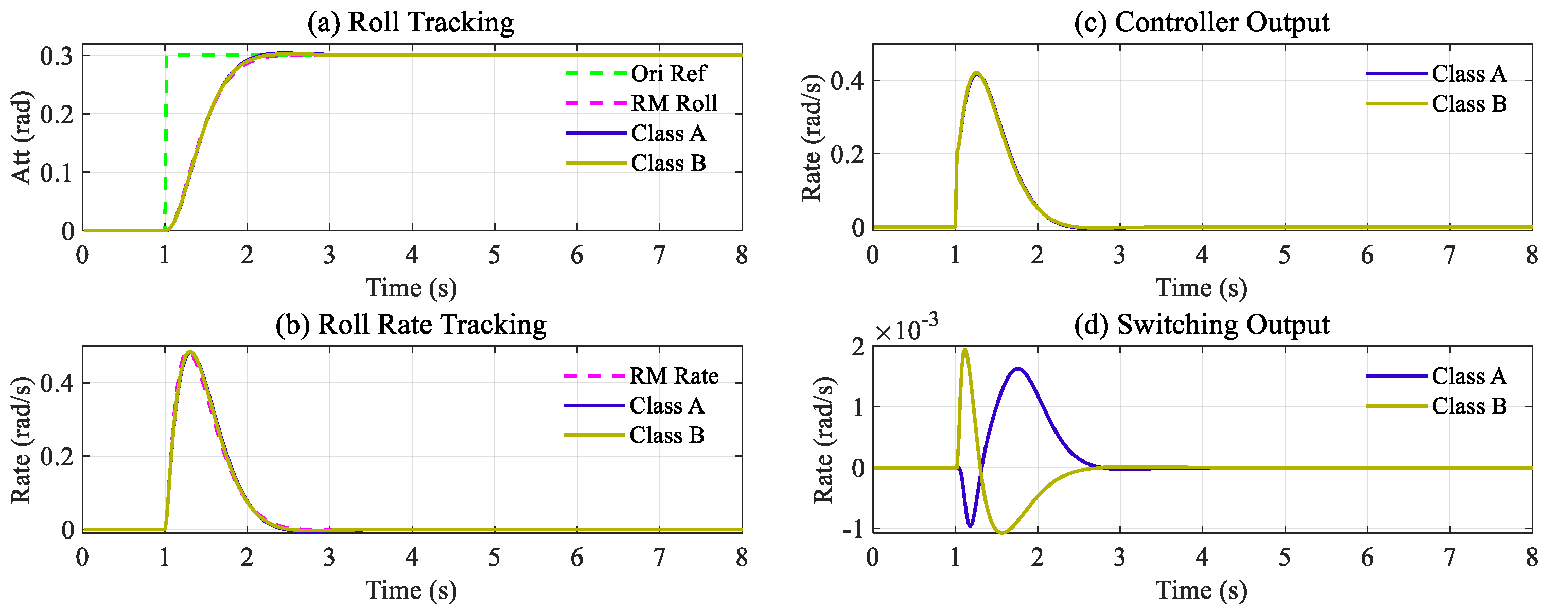
Figure 6 presents the step responses of the two improved methods after parameter tuning. The results depicted in Figure 6a,b demonstrate that both methods yield similar outcomes, with each state accurately tracking its reference target. Figure 6d displays the switching output during the tracking process; there is no chattering during tracking. Furthermore, the switching outputs exhibit comparable magnitudes. Thus, it can be concluded that both improvement methods have achieved satisfactory results for the specific system.

Figure 6 proves that the improved controller based on Class A and B can accurately track the target while avoiding chattering. In the tuning process, the same settings as in the reference studies were adopted.

In summary, this subsection compares two classic chattering reduction methods. Considering the inconsistencies of the target system, the parameter selection for each method followed the recommendations of the references. It was adjusted to the ideal state without chattering to ensure fairness in the comparison.

4.4. Simulation under Input Delay and Disturbance

Chattering is inherent in sliding mode control and appears more noticeable under input delays and external disturbances.

This section verifies the proposed method with the comparison methods in the MATLAB environment, considering the system (1), setting the attitude target of 0.3 rad based on the existing equivalent control (14), combined with the switching control calculated based on the proposed RL-based (16), the improved Class A method (30), and the improved Class B method (32), for target tracking. The system’s initial state $X={[0,0,0]}^T$.

To verify chattering suppression performance, a 20-cycle delay was performed on the controller output to imitate the actual system, which depended on the UAV’s size and maneuverability. Another factor that exacerbates chattering, the unknown disturbance, was also considered herein. Based on the delayed input, a disturbance $d\left(t\right)=0.01sin\left(t\right)$ rad was added to the system input. The response of each method and the controller output are shown in Figure 7 and Figure 8.

Figure 7 displays the target tracking performance in the presence of input delay and external disturbance, while Figure 8 records the switching output during this process. Notably, the switching outputs of all three methods exhibit the same magnitude, approximately 0.003 rad/s. Moreover, both Class A and Class B output waveforms depict similar curves, while the RL network produces a distinct curve that closely resembles a square wave, which can be considered an optimal mechanism for the current system. Finally, the tracking errors of attitudes and attitude rates for the two simulation experiments are summarized in

Table 3. Tracking result statistics under input delay and disturbance.

		Class A	Class B	Proposed
Mean	Att $\times {10}^{-3}$ (rad)	−0.825	−0.4484	−0.1214
	Rate $\times {10}^{-3}$ (rad/s)	0.7965	0.71	0.7516
Variance	Att $\times {10}^{-3}$ (rad)	0.0239	0.0223	0.0197
	Rate $\times {10}^{-3}$ (rad/s)	0.2284	0.2196	0.185

.

Compared with the initial condition, after considering input delay and disturbance, the mean errors of Class A and Class B can still be maintained. However, the attitude variance in Class A and the attitude rate variance in Class B increased by 28.5% and 48.6%, thus proving the occurrence of vibration. The proposed methods’ tracking error variance changed within 5%. Therefore, under the premise of reducing chattering, the method based on RL better tolerates system input delay.

After the increase in disturbance, the tracking effect of each method declined. Nonetheless, the chattering was still suppressed. Compared with the comparison methods, the proposed method can better reduce chattering and tolerate input delay and disturbance.

4.5. Experimental Verification

The simulated and actual environments differ significantly; hence, more than the simulation verification is needed to explain the effectiveness of the proposed method. This section presents the performance of the discussed methods on a real quadrotor, including the proposed and two classes comparison methods. During verification, each method’s environment and tracking target were consistent, and the parameters were consistent with the simulation situation.

The experiment was conducted in an outdoor natural environment, as shown in Figure 9, and the open area allowed the free flight of the UAV. A self-designed trajectory was set as the attitude target, and no human intervention was allowed during tracking.

It is worth mentioning that the controller was designed and implemented based on the fitted model; modeling errors and input delays were expected as the primary reasons for chattering. The attitude and attitude rate tracking results were recorded for evaluation, and the experimental results are shown in Figure 10, Figure 11 and Figure 12.

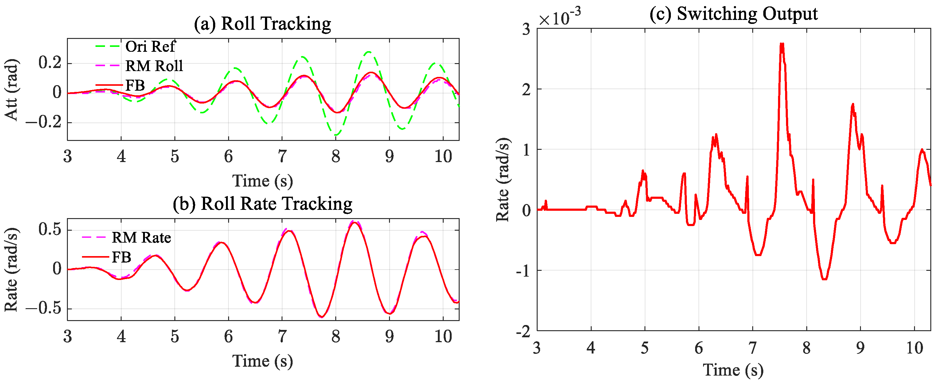
Figure 10a, Figure 11a and Figure 12a shows the designed attitude tracking performance, including the original target, reference target, and actual state feedback. Figure 10b, Figure 11b and Figure 12b shows the attitude rate tracking. Figure 10c, Figure 11c and Figure 12c shows the switching output of each method. Since the equivalent control part is entirely consistent, the switching output has better significance.

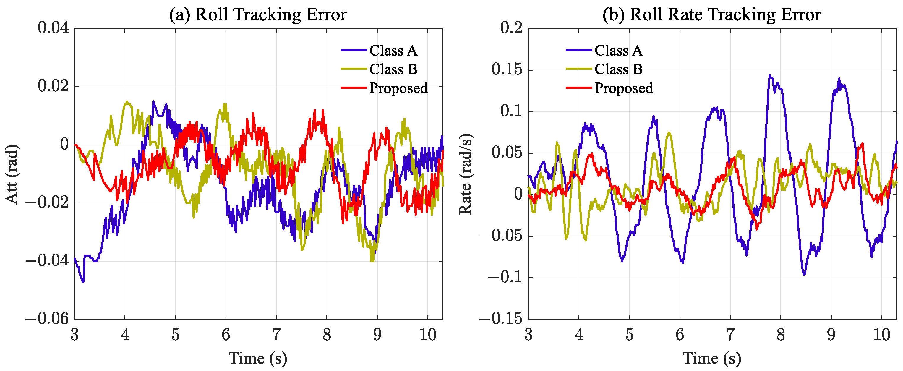
Based on the experimental results, it is evident that all three methods effectively track the planned reference attitude and rate. However, the distinct output of the switching output reveals notable differences among the three methods. Figure 10c shows that the switching output amplitude of Class A improved by 0.02 rad/s, which has a significantly larger magnitude than the other two. Nonetheless, compared with other methods, Class A improvement was the least satisfactory, and a distinct tracking error was observed. To more clearly reflect the experimental results, the tracking errors of attitude and rate are shown separately in Figure 13, and the statistical results are listed in

Table 4. Target tracking experiment result.

		Class A	Class B	Proposed
Mean	Att (rad)	−0.0174	−0.0069	−0.0045
	Rate (rad/s)	0.0167	0.0118	0.0074
Variance	Att $\times {10}^{-4}$ (rad)	0.2640	0.1340	0.0950
	Rate (rad/s)	0.0036	0.0005	0.0005
ISE	Att $\times {10}^{-3}$ (rad)	5.5	1.8	1.1
	Rate $\times {10}^{-3}$ (rad/s)	37.9	6.5	5.8

. It is worth noting that a new evaluation mechanism, the integral square error (ISE) [37,38], was adopted to evaluate the experimental results further; therefore, experiment results can be judged from different indicators.

The comparison is depicted in Figure 13a,b, it is evident that the proposed method exhibits the smallest tracking error for both attitude and rate, particularly in 3–6 s. This conclusion is further supported by the statistical results presented in Table 4. According to the statistical results in Table 4, during the actual flight, the target tracking error’s mean value, variance, and ISE of the proposed method were smaller than the two comparison methods. Therefore, it can be considered that the RL-based method achieves better tracking accuracy and stability. Additionally, it is noteworthy that none of the three schemes experienced chattering during flight.

Thus, according to the actual flight verification, the proposed improved reference sliding mode controller based on RL can reduce chattering and accurately track the attitude and attitude rate target.

5. Conclusions

This study proposed a reinforcement learning-based method to reduce chattering in sliding mode control. The DDPG algorithm was employed to learn the switching output in the sliding mode control based on a standard reference model. The reward function was designed based on the tracking errors of attitude and attitude rate. Simulation and actual flight experiments demonstrated the excellent performance of the proposed method in terms of chattering reduction and accurate tracking. Additionally, two classic chattering reduction solutions were implemented to improve the same basic controller for comparison. The proposed method effectively reduced chattering while maintaining superior tracking performance, even under conditions of input delay and disturbances.

It should be noted that reinforcement learning-based methods can avoid the design process of nonlinear controllers and their parameter selection; however, the training results may exhibit incompletely consistent properties. This study did not consider position information, which will be addressed in future research. Additionally, the current study did not account for the stability of the controller during the learning process. Future investigations will focus on incorporating stability proofs and adding constraints during training to address this issue.

References

- Miranda-Colorado, R.; Aguilar, L.T. Robust PID control of quadrotors with power reduction analysis. ISA Trans. 2020, 98, 47–62. [Google Scholar] [CrossRef]
- Matthews, M.T.; Yi, S. Neural Network Based Adaptive Flight Control of UAVs. In Proceedings of the SoutheastCon 2021, Atlanta, GA, USA, 10–13 March 2021; pp. 1–7. [Google Scholar]
- Liu, H.; Suzuki, S.; Wang, W.; Liu, H.; Wang, Q. Robust Control Strategy for Quadrotor Drone Using Reference Model-Based Deep Deterministic Policy Gradient. Drones 2022, 6, 251. [Google Scholar] [CrossRef]
- Wang, Y.; Sun, J.; He, H.; Sun, C. Deterministic Policy Gradient With Integral Compensator for Robust Quadrotor Control. IEEE Trans. Syst. Man Cybern. Syst. 2020, 50, 3713–3725. [Google Scholar] [CrossRef]
- Chen, D.; Qian, K.; Liao, K.; Zhu, Y. Research on Four-Rotor UAV Control System Based on Fuzzy Control. In Proceedings of the 2021 IEEE 5th Advanced Information Technology, Electronic and Automation Control Conference (IAEAC), Chongqing, China, 12–14 March 2021; pp. 2467–2472. [Google Scholar]
- Al-Mahturi, A.; Santoso, F.; Garratt, M.A.; Anavatti, S.G. A Robust Self-Adaptive Interval Type-2 TS Fuzzy Logic for Controlling Multi-Input–Multi-Output Nonlinear Uncertain Dynamical Systems. IEEE Trans. Syst. Man Cybern. Syst. 2022, 52, 655–666. [Google Scholar] [CrossRef]
- Rabah, M.; Haghbayan, H.; Immonen, E.; Plosila, J. An AI-in-Loop Fuzzy-Control Technique for UAV’s Stabilization and Landing. IEEE Access 2022, 10, 101109–101123. [Google Scholar] [CrossRef]
- Prach, A.; Kayacan, E. An MPC-based position controller for a tilt-rotor tricopter VTOL UAV. Optim. Control Appl. Methods 2018, 1, 343–356. [Google Scholar] [CrossRef]
- Ahmed, S.; Wang, H.; Tian, Y. Adaptive High-Order Terminal Sliding Mode Control Based on Time Delay Estimation for the Robotic Manipulators with Backlash Hysteresis. IEEE Trans. Syst. Man Cybern. Syst. 2021, 51, 1128–1137. [Google Scholar] [CrossRef]
- Lian, S.; Meng, W.; Shao, K.; Zheng, J.; Zhu, S.; Li, H. Full Attitude Control of a Quadrotor Using Fast Non-singular Terminal Sliding Mode with Angular Velocity Planning. IEEE Trans. Ind. Electron. 2022, 4, 3975–3984. [Google Scholar]
- Chen, H.; Shao, X.; Xu, L.; Jia, R. Finite-Time Attitude Control with Chattering Suppression for Quadrotors Based on High-Order Extended State Observer. IEEE Access 2021, 9, 159724–159733. [Google Scholar] [CrossRef]
- Liu, K.; Wang, R. Antisaturation Adaptive Fixed-Time Sliding Mode Controller Design to Achieve Faster Convergence Rate and Its Application. IEEE Trans. Circuits Syst. II Express Briefs 2022, 69, 3555–3559. [Google Scholar] [CrossRef]
- Wang, W.; Nonami, K.; Hirata, M.; Miyazawa, O. Autonomous control of micro flying robot. J. Vib. Control 2010, 16, 555–570. [Google Scholar] [CrossRef]
- Li, D.; Yu, H.; Tee, K.P.; Wu, Y.; Ge, S.S.; Lee, T.H. On time-synchronized stability and control. IEEE Trans. Syst. Man Cybern. Syst. 2021, 52, 2450–2463. [Google Scholar] [CrossRef]
- Utkin, V.; Lee, H. Chattering Problem in Sliding Mode Control Systems. In Proceedings of the International Workshop on Variable Structure Systems, 2006. VSS’06, Alghero, Sardinia, 5–7 June 2006; pp. 346–350. [Google Scholar]
- Matouk, D.; Abdessemed, F.; Gherouat, O.; Terchi, Y. Second-order sliding mode for Position and Attitude tracking control of Quadcopter UAV: Super-Twisting Algorithm. Int. J. Innov. Comput. Inf. Control 2020, 1, 29–43. [Google Scholar]
- Jayakrishnan, H.J. Position and attitude control of a quadrotor UAV using super twisting sliding mode. IFAC-PapersOnLine 2016, 1, 284–289. [Google Scholar] [CrossRef]
- Lei, W.; Li, C. An Adaptive Quasi-Sliding Mode Control Without Chattering. In Proceedings of the 2018 37th Chinese Control Conference (CCC), Wuhan, China, 25–27 July 2018; pp. 1018–1023. [Google Scholar]
- Yang, Y.; Yan, Y. Attitude regulation for unmanned quadrotors using adaptive fuzzy gain-scheduling sliding mode control. Aerosp. Sci. Technol. 2016, 54, 208–217. [Google Scholar] [CrossRef]
- Miranda-Colorado, R. Observer-based proportional integral derivative control for trajectory tracking of wheeled mobile robots with kinematic disturbances. Appl. Math. Comput. 2022, 2432, 127372. [Google Scholar] [CrossRef]
- Zhang, J.; Zhang, N.; Shen, G.; Xia, Y. Analysis and design of chattering-free discrete-time sliding mode control. Int. J. Robust Nonlinear Control 2019, 29, 6572–6581. [Google Scholar] [CrossRef]
- Xu, W.; Junejo, A.K.; Liu, Y.; Islam, M.R. Improved Continuous Fast Terminal Sliding Mode Control with Extended State Observer for Speed Regulation of PMSM Drive System. IEEE Trans. Veh. Technol. 2019, 68, 1046–10476. [Google Scholar] [CrossRef]
- Wang, W.; Ma, H.; Xia, M.; Weng, L.; Ye, X. Attitude and altitude controller design for quad-rotor type MAVs. Math. Probl. Eng. 2013, 2013, 587098. [Google Scholar] [CrossRef] [Green Version]
- Yue, W.H.; Ouyang, P.R.; Tummalapalli, M. PD with Terminal Sliding Mode Control for Trajectory Tracking. In Proceedings of the 2020 IEEE/ASME International Conference on Advanced Intelligent Mechatronics (AIM), Boston, MA, USA, 6–9 July 2020; pp. 1400–1405. [Google Scholar]
- Pan, H.; Zhang, G.; Ouyang, H.; Mei, L. A Novel Global Fast Terminal Sliding Mode Control Scheme for Second-Order Systems. IEEE Access 2020, 8, 22758–22769. [Google Scholar] [CrossRef]
- Wang, Y.; Yao, W.; Chen, X.; Ceriotti, M.; Bai, Y.; Zhu, X. Novel Gaussian mixture model based nonsingular terminal sliding mode control for spacecraft close-range proximity with complex shape obstacle. Proc. Inst. Mech. Eng. Part G J. Aerosp. Eng. 2022, 3, 517–526. [Google Scholar] [CrossRef]
- Wang, F.; Ma, Z.; Gao, H. Disturbance Observer-based Nonsingular Fast Terminal Sliding Mode Fault Tolerant Control of a Quadrotor UAV with External Disturbances and Actuator Faults. Int. J. Control Autom. Syst. 2022, 4, 1122–1130. [Google Scholar] [CrossRef]
- Zhao, K.; Jia, F.; Shao, H. A novel conditional weighting transfer Wasserstein auto-encoder for rolling bearing fault diagnosis with multi-source domains. Knowl.-Based Syst. 2022, 262, 110203. [Google Scholar] [CrossRef]
- Jin, B.; Cruz, L.; Gonçalves, N. Deep facial diagnosis: Deep transfer learning from face recognition to facial diagnosis. IEEE Access 2020, 8, 123649–123661. [Google Scholar] [CrossRef]
- Zhao, K.; Hu, J.; Shao, H.; Hu, J. Federated multi-source domain adversarial adaptation framework for machinery fault diagnosis with data privacy. Reliab. Eng. Syst. Saf. 2023, 236, 109246. [Google Scholar] [CrossRef]
- Farjadian, A.B.; Yazdanpanah, M.J.; Shafai, B. Application of reinforcement learning in sliding mode control for chattering reduction. In Proceedings of the World Congress on Engineering, London, UK, 3–5 July 2013; Volume 2. [Google Scholar]
- Guo, L.; Zhao, H.; Song, Y. A Nearly Optimal Chattering Reduction Method of Sliding Mode Control with an Application to a Two-wheeled Mobile Robot. arXiv 2021, arXiv:2110.12706. [Google Scholar]
- Li, B.; Li, Q.; Zeng, Y.; Rong, Y.; Zhang, R. 3D trajectory optimization for energy-efficient UAV communication: A control design perspective. IEEE Trans. Wirel. Commun. 2021, 21, 4579–4593. [Google Scholar] [CrossRef]
- Wang, Q.; Wang, W.; Suzuki, S.; Namiki, A.; Liu, H.; Li, Z. Design and Implementation of UAV Velocity Controller Based on Reference Model Sliding Mode Control. Drones 2023, 7, 130. [Google Scholar] [CrossRef]
- Noormohammadi-Asl, A.; Esrafilian, O.; Arzati, M.A.; Taghirad, H.D. System identification and H-infinity-based control of quadrotor attitude. Mech. Syst. Signal Process. 2020, 135, 106358. [Google Scholar] [CrossRef]
- Lillicrap, T.P.; Hunt, J.J.; Pritzel, A.; Heess, N.; Erez, T.; Tassa, Y.; Silver, D.; Wierstra, D. Continuous control with deep reinforcement learning. arXiv 2015, arXiv:1509.02971. [Google Scholar]
- Liu, K.; Wang, R.; Zheng, S.; Dong, S.; Sun, G. Fixed-time disturbance observer-based robust fault-tolerant tracking control for uncertain quadrotor UAV subject to input delay. Nonlinear Dyn. 2022, 107, 2363–2390. [Google Scholar] [CrossRef]
- Liu, K.; Wang, R.; Wang, X.; Wang, X. Anti-saturation adaptive finite-time neural network based fault-tolerant tracking control for a quadrotor UAV with external disturbances. Aerosp. Sci. Technol. 2021, 115, 106790. [Google Scholar] [CrossRef]
Figure 1.
System structure of the RL–based reference model SMC.
Figure 2.
Schematic diagram of the training process.
Figure 3.
Quadrotor platform.
Figure 4.
Cumulative rewards during training.
Figure 5.
Tracking performance: Comparing the conventional SMC with the proposed controller: (a) roll tracking, (b) roll rate tracking, and (c) controller output of the two methods. Evidently, the proposed method significantly reduces chattering.
Figure 6.
Step response based on Class A and Class B improvement: (a,b) depict the accurate tracking of the target attitude and rate for the two improved methods; (c) illustrates the total controller outputs, and (d) represents the switching output. The output assignments of the two methods are similar, indicating comparable performance between them.
Figure 7.
Target tracking under delayed input and disturbance.
Figure 8.
Controller output under delayed input and disturbance.
Figure 9.
Quadrotor flight experiment in a natural environment.
Figure 10.
Target tracking experiment results of Class A improvements.
Figure 11.
Target tracking experiment results of Class B improvements.
Figure 12.
Target tracking experiment results of the proposed improvements.
Figure 13.
Tracking error in the four methods.