Hyper-Local Weather Predictions with the Enhanced General Urban Area Microclimate Predictions Tool

Abstract

This paper presents enhancements to, and the demonstration of, the General Urban area Microclimate Predictions tool (GUMP), which is designed to provide hyper-local weather predictions by combining machine-learning (ML) models and computational fluid dynamic (CFD) simulations. For the further development and demonstration of GUMP, the Embry–Riddle Aeronautical University (ERAU) campus was used as a test environment. Local weather sensors provided data to train ML models, and CFD models of urban- and suburban-like areas of ERAU’s campus were created and iterated through with a wide assortment of inlet wind speed and direction combinations. ML weather sensor predictions were combined with best-fit CFD models from a database of CFD flow fields, providing flight operational areas with a fully expressed wind flow field. This field defined a risk map for uncrewed aircraft operators based on flight plans and individual flight performance metrics. The potential applications of GUMP are significant due to the immediate availability of weather predictions and its ability to easily extend to arbitrary urban and suburban locations.

1. Introduction

Advanced Air Mobility (AAM) is an emerging air transportation system that promises to move both people and cargo in a more efficient and ecologically friendly manner within and between urban areas while connecting these urban areas to adjacent suburban and rural locales [1]. AAM stakeholders ultimately envision hundreds-to-thousands of simultaneous flight operations in support of this vision over and around large metropolitan areas. Flight operations will consist of a mix of different aircraft types to serve the niche markets (e.g., cargo transportation, people transport, aerial work) composing the broader AAM ecosystem. Associated aircraft will span in size from smaller parcel-delivering aircraft operating in low altitude airspace (Uncrewed Aircraft Systems (UAS) Traffic Management (UTM)) to larger aircraft transporting people and cargo at slightly higher altitudes in a more traditional Air Traffic Management (ATM) setting. Collectively, these vertically stacked operations will predominately take place in a block of altitudes stretching from the surface to 5000 feet above ground level (AGL), with larger AAM aircraft cruising at nominal altitudes of 1000–2000 feet AGL [2,3,4,5,6]. This block of altitude composes the atmospheric boundary layer (ABL), a spatially and temporally dynamic portion of the atmosphere that is also characterized by persistent turbulence [7]. With many AAM operations tailored for the urban environment, a large number of operations will take place within the urban boundary layer (UBL), a portion of the ABL that is influenced by the presence of a city [8]. Since the properties of the UBL tend to reflect those of the underlying surface, which hosts more roughness elements (e.g., buildings) and possesses more surface cover heterogeneity (e.g., asphalt, concrete, grass and other natural and artificial surfaces), the UBL tends to be an even more dynamic environment than the general ABL found over more rural, homogeneous outlying areas. This lower portion of the atmosphere (i.e., the ABL) has traditionally been an environment that aircraft have quickly passed through during departure- and approach-flight segments. However, with the advent of AAM, a new era of sustained aviation operations is envisioned in this dynamic portion of the atmosphere, and, consequently, new forecasting products need to be developed.

Within the AAM ecosystem, small UASs (sUAS) will play a central role in small package delivery and aerial work, such as the last-mile delivery of parcels and medical supplies, infrastructure inspection, and search-and-rescue, respectively. These sUAS operations are envisioned to occur in the UTM environment below 400 feet AGL. Consequently, these aerial vehicles will not only be operating in a new and dynamic environment but, because of their decreased size, mass, thrust and speed, they will also be more susceptible to their environment. This makes timely and reliable hyperlocal forecasting for this environment essential, and these sUAS operations are the ones in which this work seeks to support.

To date, efforts toward hyperlocal forecasting have been rather limited. Common strategies that have been employed for this include running large-scale Numerical Weather Prediction (NWP) models with smaller grid cells that provide increased spatial resolution [9,10]. However, the increased number of calculations on these finer grids make them impractical for real-time forecasting with currently available computational resources. Computational Fluid Dynamics (CFD) has been used in conjunction with highly detailed urban and topographical models to predict boundary layer flow patterns [11,12,13] and for applications that include plume dispersion and the spread of airborne toxins [14,15], predicting wind loads on buildings [16,17], assessing the wind resource for urban wind energy generation [18,19,20], and investigating urban pedestrian comfort [21,22]. However, similarly to the large-scale NWP run on fine grids, the associated computational costs for these applications are appropriate for one-off analysis but not for real-time weather forecasting. Finally, the downscaling of large-scale NWP on finer grids has been used with the incorporation of additional strategically placed sensors [23,24]. While this strategy has great potential for hyperlocal forecasting, the requirement for deliberately placed specialized sensors limits the utility of this methodology. The General Urban Area Microclimate Predictions Tool (GUMP) [25] was developed with this need and these challenges in mind. This work reports on the expansion of GUMP capability and its validation via observations made within representative urban and suburban environments on Embry–Riddle Aeronautical University’s (ERAU) campus.

The following section of this paper is broken down into two main segments. Section 2.1 provides an overview of GUMP, including the associated machine-learning forecasting and the iterative inference schemes using CFD. Section 2.2 details the experimental field campaign using sUAS. Section 3 of this work juxtaposes the GUMP model output with the empirical observations. Following these results, the promising utility of GUMP for sUAS operations is discussed, while also highlighting strategies for improvement. Finally, a summary of the work is provided and additional applications for GUMP are suggested.

2. Methodology

2.1. GUMP Overview

GUMP is a micro-scale, hyper-local weather prediction service for rural and urban areas, and it leverages mesoscale forecasts in combination with data from local weather sensors and CFD-derived datasets. GUMP combines the benefits of high-fidelity CFD with the prediction capability of machine-learning (ML) models while targeting the specific needs of sUAS operators. Toward this, GUMP has two major components (Figure 1): forecasting for estimating future weather at specific point locations by consuming live and forecast data from the National Oceanic and Atmospheric Administration (NOAA), along with other sources, and creating temporal predictions using ML models; and iterative inference for extending these estimates to all other points within the area of interest using selective CFD simulations [25].

2.1.1. Machine-Learning Forecasting

ML models were trained using past data collected by local weather stations. For example, data were collected from ERAU’s weather stations (“0104W”, “E5900”, “E9392”, and “F3022”) from August 2019 to January 2022, and then used to train the models. It should be noted that the reporting frequency for these stations was every 10 min.

Each individual ML model is a recurrent neural network (RNN) with the same general structure, although hyperparameters can be set for the long short-term memory (LSTM) layer dropout fraction, the dense layer dropout fraction, the final layer activation function, the loss function, and the number of nodes in the LSTM layers. For the ERAU sensor datasets, notional hyperparameters are selected as initial values based on the relative dataset sizes. Additionally, hyperparameter tuning was performed to optimize the performance of the ML models. The forecast weather (wind speed and wind direction) from the ML models is generated for one-to-six hours into the future, based on the most recent six hours of measurements. Representative results are shown in Figure 2, which use WeatherStem mesonet data [26]. As anticipated, the overall trend shows that the prediction error increases with a longer forecast horizon, which is expected since more immediate weather conditions are easier to predict than those that are further into future. For wind speed, 80% of the predictions are within 1 m/s. The error, albeit small, fluctuates widely for the first hour of the time horizon but subsequently stabilizes. In contrast, the wind direction error appears to increase at a constant rate for the entirety of the six-hour prediction horizon. Median errors in wind direction prediction are modest (<30°) for the entire prediction horizon.

2.1.2. Iterative Inference Using CFD

To expand GUMP’s application to diverse geographic regions of interest, a model of the ERAU campus was created and divided into four sections (Figure 3). Treating these sections as individual wind flow regions allowed for the production of a modular wind field database, which provides a flow field throughout the entire area of interest.

Steady-state CFD modeling is dependent on the boundary conditions provided for the simulation, including domain geometry and flow boundaries. By changing the flow inlet conditions to capture variations in wind speed and direction, a sweep across many potential wind fields was performed by rotating the inlet face around the domain; the south wind configuration is shown in Figure 4. A total of 720 cases were evaluated via the ANSYS Fluent CFD solver using the k-epsilon Reynolds-averaged Navier–Stokes (RANS) solver [25]. This turbulence model was used for its low computational cost compared to other solvers, such as unsteady Reynolds-averaged Navier–Stokes (URANS) or large eddy simulations (LES). For the formulation of flight plans, the transient effects from an unsteady flow simulation are of a lower priority (assuming turbulent areas are sufficiently identified). While LES would provide better quality in the output models, most of the effects that RANS is unable to capture occur close to the walls. We do not expect aircraft to be flying here; hence, those predictions are not critical. The convergence criteria defined is 1 × 10⁻⁴, and the models were run at steady state for a maximum of 10,000 iterations. Mesh refinement was performed to meet the convergence criteria by applying cell-sizing constraints.

The evaluated cases were derived from all possible combinations of the five computer-aided design (CAD) models (four sections and the entire campus), nine flow speeds ranging from four knots to 36 knots in four-knot increments, and 16 flow angles ranging from 0° to 360° in 22.5° increments. The full campus model was included in these sweeps to provide additional resources for evaluating the performance of future model approximations. Possessing many variations in wind flow for individual subsections of the location of interest improved the potential for local wind prediction, as separate sections were allowed to vary on the specific CFD case deemed to fit the best.

The large number of simulation cases were conducted by leveraging the built-in simulation automation capabilities of ANSYS via its journaling feature. The meshing parameters applied to each case were the same: a mesh cell of 4 m was used for modeling the buildings, while 50 m was used for the ground, an example of which is shown in Figure 5. The large number of CFD cases captured a reasonable array of expected wind conditions. Whereas more cases would always be preferred from an accuracy perspective, additional cases can significantly increase computational costs of the CFD simulations, as well as their subsequent integration with the ML models. Consequently, this approach is scalable in terms of expanding the dataset while reducing repeated computational overhead where possible.

The flow conditions at a desired location (or sensor) are estimated by comparing the observed initial flow condition at the desired location with the database of CFD simulation results and determining the simulation case with the best match. A lookup function was developed to automatically implement this comparison process. However, this strategy is only relevant if accurate initial condition information can be ascertained at the desired location, such as the case when a weather sensor provides accurate information for that exact location. For cases when this is not possible, such as locations that either lack a sensor input and are, therefore, ineligible for the previously defined lookup function, or where the lookup function returns multiple potential matches, inferences are made to assign an appropriate flow field. For areas where an inference cannot be made with the provided data, additional iterations of the inference scheme can propagate sensor information to the lacking locations while maintaining deference to available sensor data. Toward meeting this challenge, an iterative inference scheme is developed.

The iterative inference scheme uses the boundaries between two adjacent sections of a geographic region, in this case covering the ERAU campus, to choose the best CFD result. An example of the iterative inference was generated by assuming an input prediction of southerly wind flow at 8 m/s at the 0104W sensor. Using this sensor input, a wind field model was produced for the entire ERAU campus (Figure 6). The four section models used to produce this flow field were derived from CFD results with inlet conditions corresponding to a southerly wind. The selected upper right section was derived from a far field wind of 4 m/s, which was slower than expected and produced more noticeable discontinuities in wind speeds along a horizontal boundary on the right side. This was likely due to the positioning of the sensor downstream from obstructions in the flow slowing down the freestream velocity. Discontinuities between individual sections in the completed flow field are expected and minimized by using boundary comparisons to help select wind field combinations based on the lowest discrepancy in wind vectors.

2.1.3. User Interface

The GUMP tool has been integrated into a data pipeline that ingests live weather data and outputs detailed predicted flow fields for several hours into the future and displays this on a live interface. An example of this display is shown in Figure 7. The flight plan is demonstrated by bold arrows embedded in purple that, in this case, navigated through the center of ERAU’s campus. Wind vectors throughout the flight operation area are color-coded according to wind speed. While color assignment is configurable, in this case, red vectors are assigned to wind speeds over 20 mph, which may be of concern to sUAS operators. Several dominant wind corridors are observable, as well as changes in wind speed over and around buildings. It is quite possible in this scenario that the proposed flight route is unsuitable at this forecasted time. Providing this information to the operator will make the deployment of the sUAS safer with the knowledge that there are wind magnitudes that may exceed the capabilities of the sUAS. This can prevent a circumstance that may result in a flight mishap that endangers people or property in the area.

2.2. sUAS Flight Operations

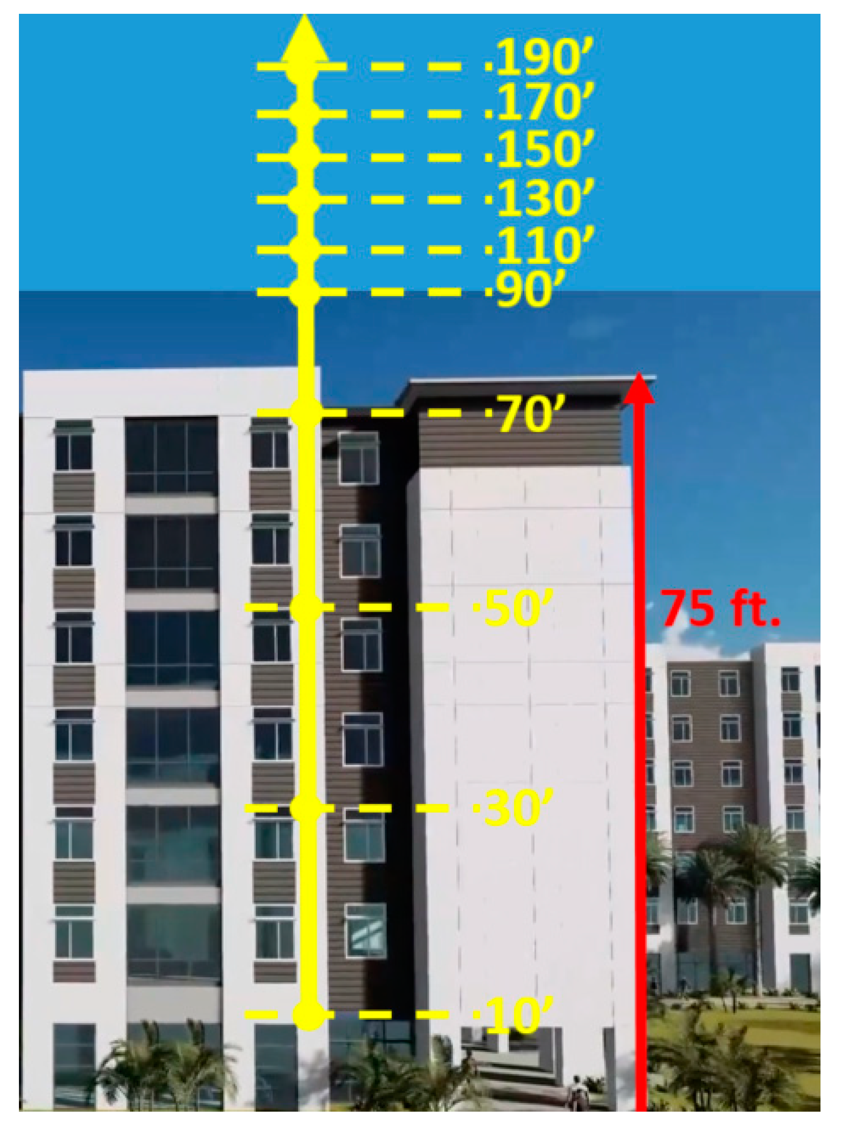
2.2.1. Experimental Setting

With the availability of historical weather data, presence of requisite surface sensors, topographical insight, and proximity to the flight operation team’s location, among other factors, ERAU’s Daytona Beach campus was identified as the primary demonstration site. To further develop the capability to forecast for arbitrary regions of interest, a model of the ERAU campus was created, as previously mentioned. ERAU’s central campus offers both mid-rise buildings (seven floors) that reflect modern urban architecture and a building density that enables it to serve as a proxy for an urban setting, including an urban canyon (a setting of much interest and concern for urban sUAS operations). ERAU’s athletic complex, adjacent to its central campus, consists of numerous athletic fields and a broad area with a lower density of roughness elements. This provided the setting for a proxy suburban flight operational area.

ERAU’s campus sits adjacent to Daytona Beach International Airport (KDAB). The proximity of ERAU’s representative urban and suburban environments to KDAB enabled GUMP development and validation in a real-world scenario consisting of a hub and spoke distribution network. Here, KDAB serves as a hub style product distribution center. For an urban delivery scenario, a sUAS follows a route from the proxy distribution center to a package destination situated within a cluster of seven-story residence halls (Figure 8). The entirety of the flight occurs with the roughness sublayer, and the delivery location is located at the end of an urban canyon (Figure 9). A similar “suburban” last-mile delivery scenario was created by a flight plan that began at the same package delivery hub, passed through Embry–Riddle’s central campus, and terminated in Embry–Riddle’s athletic complex, itself sitting adjacent to a suburban neighborhood (Figure 10). Due to flight restrictions stemming from the demonstration area’s close proximity to KDAB, a Certificate of Waiver or Authorization (COA) was obtained from the Federal Aviation Administration (FAA) in order to conduct the flight operations.

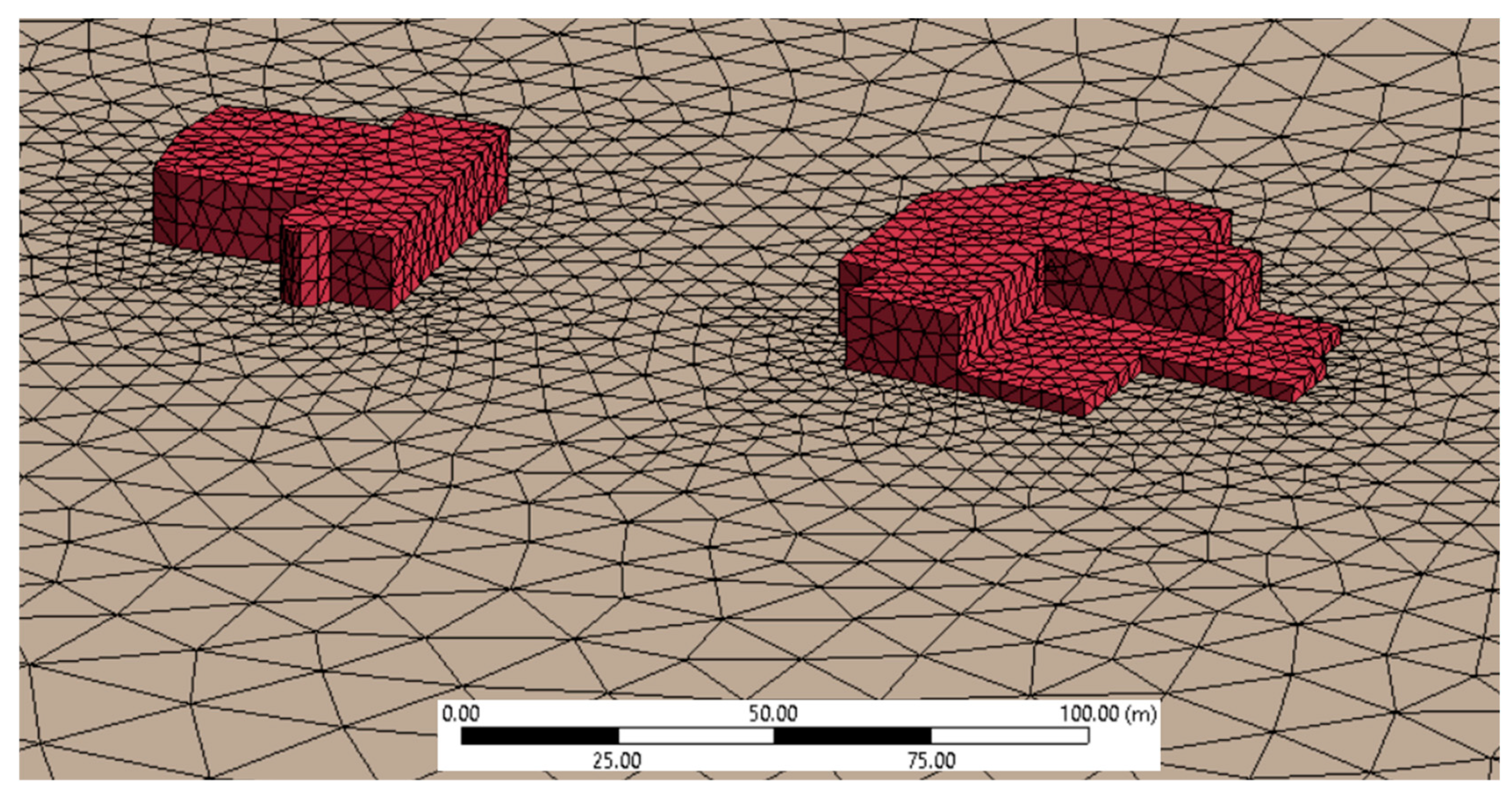
2.2.2. Creation of the Built Environment Model

To enable the creation of the large array of CFD simulation cases, a mesh of the built environment had to be constructed for execution of the numerical simulations. LiDAR and photogrammetry serve as a means for rapidly, and accurately, creating virtual models of real-world objects. UAS with ultra-precise flight path control are ideal platforms for moving cameras and LiDAR sensors in such an environment and were used to create a 3D model of ERAU’s campus.

Imaging and creating virtual buildings using photogrammetric techniques involves several steps [27]. First, a UAS flight plan is programmed that provides a desired ground sampling distance (GSD). GSD is determined by the distance between two consecutive pixel centers in a selected image. The smaller the value of the image GSD, the higher the degree of spatial resolution for the image. Lower values of GSD lead to increased levels of visible detail. The UAS captured images that were automatically geotagged in the Exchangeable Image File Format (exif) by software that reads positional information from the UAS. This tagging provides the necessary positional accuracy required during post-processing. Photogrammetric software then stitches together discrete images using parallactic measurements, thus allowing for the creation of virtual 3D models.

LiDAR was also incorporated for the remote sensing (i.e., accurate measurement and geolocating of surfaces and features) of buildings within the demonstration area. Similar to photogrammetry, the workflow for UAS-borne LiDAR also begins with programming a flight path that considers the altitude of the UAS, speed of the UAS, overlap of data collection paths, and transitions between flight paths [28]. The LiDAR used for this project [29] produced superior results when flown at an altitude of 140 feet AGL and at a speed of 5 mph. This speed and altitude enabled creation of a dense LiDAR point cloud with up to 400 points per square meter.

Post-processing of both photogrammetrically and LiDAR produced densely populated 3D point clouds allowed creation of triangle meshes, which served as the framework for the virtual objects with photo-real textures. The triangle meshes were refined, using Autodesk 3ds Max [30], into .obj- and .fbx-formatted virtual objects. These formats are widely interchangeable with numerous programs (e.g., flight simulation and CAD). The resulting 3D model is shown in Figure 3.

2.2.3. Observations by Meteorologically Instrumented sUAS

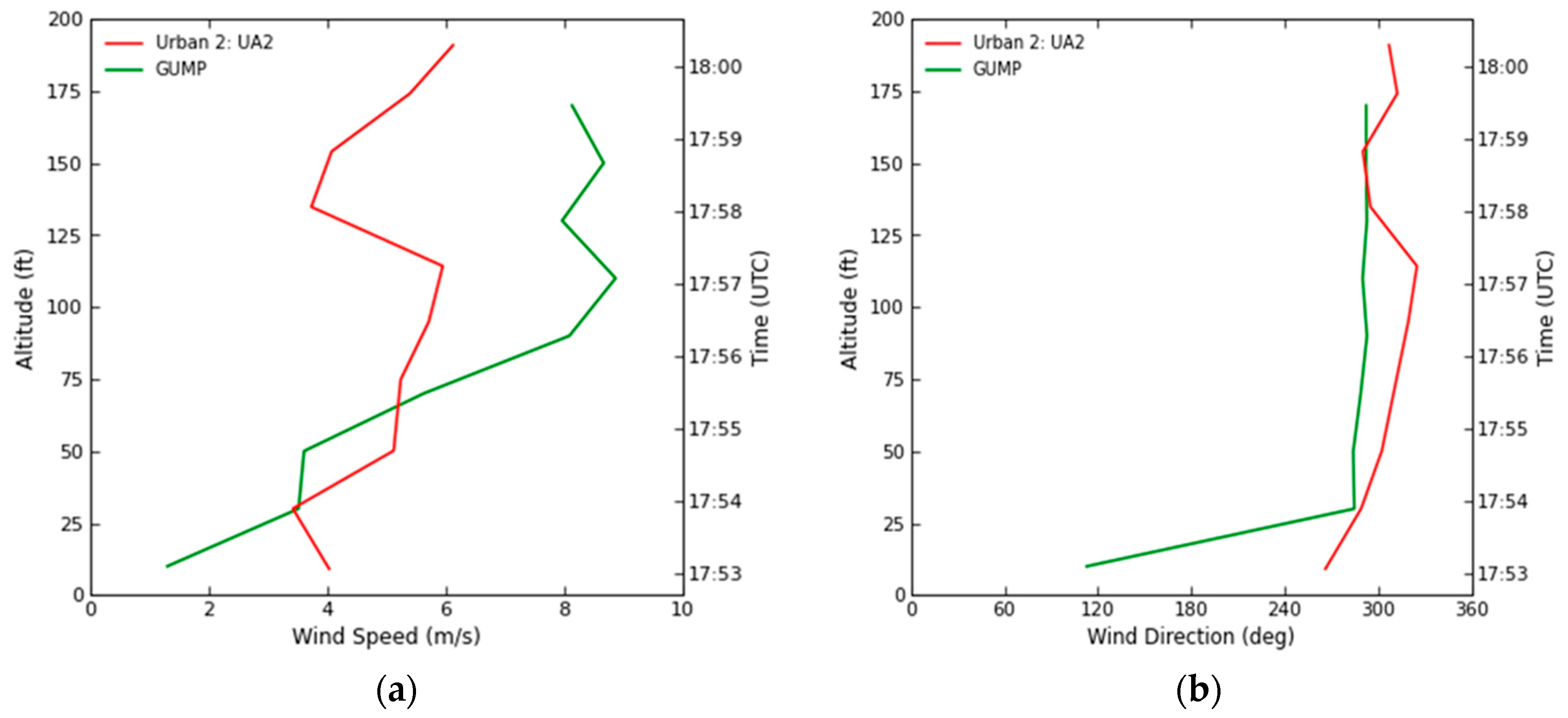
Two meteorologically instrumented multirotor (MR) sUASs were employed to make observations along both the urban and suburban routes. MR sUASs were chosen for their ability to obtain measurements in a continuous manner, or along a discontinuous route, at deliberately chosen points of interest. The ability to hover also provides the opportunity to obtain longer data records and to respect the response times of each sensor. Thermodynamic observations were made with a resistance temperature detector (RTD) to obtain temperature and a capacitive humidity sensor for relative humidity. Barometric pressure was ascertained from a micro-electro-mechanical system (MEMS) pressure sensor. Wind speed and direction were measured by an ultrasonic anemometer making use of acoustic resonance technology. Data were written locally on the sUAS while simultaneously being telemetered in order to mitigate risk by continuously monitoring the dynamic flight environment and in order to empower real-time decision-making. One of the meteorologically instrumented MR sUASs is displayed hovering in Figure 11.

Flight observations, for validating numerical simulation results, were conducted on a moderately windy day and spanned from the late morning, with a well-mixed ABL to the evening transition. The instrumented sUAS were laterally staggered roughly 100 feet apart and flew simultaneous ascending vertical profiles from 10 feet to 190 feet AGL. Thirty-second data records were obtained while in a hover at 20-foot intervals. Thus, this provided 10 distinct observations per vertical profile (Figure 12). Subsequent to accomplishing a set of vertical profiles, the pair of sUASs was advanced further down the delivery route. The location of the vertical profiles along each route is displayed in Figure 13.

3. Results

For validation, high-resolution GUMP model output was compared to in-situ observations made by the instrumented sUAS. For the purpose of observational data quality, only measurements made during ascent were recorded to ensure that observations were conducted in undisturbed air. Therefore, the lowest and highest altitude for a given vertical profile marked the beginning and end of the data record, respectively. Representative comparisons between model output and observations for a vertical profile that lies on the flight route are shown in Figure 14 and Figure 15. Figure 14 is a comparison of sUAS 1 observations and GUMP output, with the corresponding comparison for sUAS 2 shown in Figure 15. For these comparisons, vertical profiles accomplished from 1753–1800 UTC are shown in red. For comparison, the GUMP model timeframe for 1730–1739 UTC was chosen (green). With a GUMP model forecast horizon of 20 min, the model output for this time period was equivalent to the time period of the sUAS profiles.

GUMP performed well when predicting wind speeds at the lower altitudes but overestimated wind speeds at the upper altitudes for both sUAS flight profiles. With the exception of the lowest bin at sUAS 2′s location, GUMP performed extremely well in forecasting wind direction. In general, Figure 14 and Figure 15 are indicative of GUMP’s overall performance, forecasting wind magnitude better at lower altitudes but overpredicting wind speed at higher heights while handling wind direction well.

The analysis captured in Figure 14 and Figure 15 is based on a 20-min time horizon, as if a flight operation is imminent. Since the accuracy of the ML predictions improve as the forecasted time approaches, a separate review of the tool’s performance in the hours leading up to a flight operation, when more preliminary planning might be underway, is also of interest.

Table 1. sUAS wind speed measurements at 30 ft. compared to GUMP urban and suburban forecasts for the same altitude. The GUMP forecast values are an average of the 12 forecasts made from two hours prior to the sUAS flights. All values given in m/s.

Scenario	sUAS 1	sUAS 2	GUMP (2-h Average)	GUMP— sUAS1	GUMP— sUAS2
Urban 1	3.07	0.83	4.96	1.89	4.13
Urban 2	4.69	3.43	4.65	−0.04	1.22
Urban 3	2.46	3.25	4.72	2.26	1.47
Urban 4	2.22	3.56	4.82	2.60	1.26
Suburban 1	3.95	4.38	1.81	−2.14	−2.57
Suburban 2	1.19	1.03	2.11	0.92	1.08
Suburban 3	4.33	3.66	2.41	−1.92	−1.25
Suburban 4	2.23	2.21	2.65	0.42	0.44
Suburban 5	4.00	4.12	2.47	−1.53	−1.65

(magnitude) and

Table 2. sUAS wind direction observation at 30 ft. compared to GUMP urban and suburban forecasts for the same altitude. The GUMP forecast values are an average of the 12 forecasts made from two hours prior to the sUAS flights. All values given in degrees.

Scenario	sUAS 1	sUAS 2	GUMP (2-h Average)	GUMP— sUAS1	GUMP— sUAS2
Urban 1	214.05	212.61	300.78	86.73	88.17
Urban 2	299.41	289.22	282.38	−17.03	−6.84
Urban 3	323.59	314.05	284.58	−39.01	−29.47
Urban 4	297.24	308.43	305.04	7.80	−3.39
Suburban 1	282.27	282.26	275.17	−7.10	−7.09
Suburban 2	270.48	294.81	291.92	21.44	−2.89
Suburban 3	306.84	310.34	297.52	−9.32	−12.82
Suburban 4	310.80	286.57	304.11	−6.69	17.54
Suburban 5	301.71	313.47	296.05	−5.66	−17.42

(direction) compare observations taken by sUAS 1 and sUAS 2 with GUMP forecasts at 30 feet AGL along both the urban and suburban routes. Forecast output and observations are compared across nine locations along the flight routes, including four locations in the urban region and five locations in the suburban region. The sUAS wind speeds represent the average of 30 s of data observed at 30 feet for the associated region. The contrasting GUMP output is the average value of 12 10-min periods of GUMP forecasts for two hours prior to the sUAS flights. Each table represents the differences between forecast and observed winds: shades of blue indicate model overestimation, whereas shades of red indicate an underestimation.

Overall, Table 1 and Table 2 show that GUMP overestimated wind speed and underestimated wind direction in the urban setting, with the singular exception of the large difference in wind direction for the Urban 1 scenario. The suburban forecasts were much more likely to result in an underestimation for both sUAS locations. Overall, the suburban forecasts were more accurate than the urban forecasts.

4. Discussion

GUMP’s inaugural demonstration shows promising utility for sUAS operations while also pointing toward strategies for improvement. Unsurprisingly, forecasts along the suburban corridor resulted in better prediction accuracy, likely due to the lower number of flow obstructions and the resulting simplified fluid dynamics. However, GUMP’s ability to more accurately predict wind direction possibly emphasizes the importance and varying impact of upstream flow effects.

The higher accuracy in wind predictions observed at lower altitudes is expected due to the nature of the CFD selection process. The flow fields chosen to define the target area are selected based on similarity to a predicted wind vector at the known sensor location. Since the wind sensor used for the presented results is approximately 8 m above the ground, this is the level where the highest accuracy would be anticipated, and results confirmed this. This underscores the limitation of relying on a single sensor source for the selection process. Presumably, forecasting improvement would be realized with additional strategically placed sensors (laterally and vertically) for use in fitting the CFD models to the predictions/sensor readings.

Closely tied to the issue of the number of sensors is the increased attention that must be given to sensor placement and setup. One of the sensors used here was atop a building, which may impact the flow field and, thus, create unrepresentative observations. This can render the resulting data unsuitable for multiple flow fields within close proximity. Each of these sensor issues can degrade GUMP performance through both the quality of the ML training data and the determination of the best matched simulation case.

Consequently, moving forward, there are required improvements for GUMP to increase its accuracy, usability, and deployability. The aforementioned sensor issues can be rectified by more purposely chosen and sited sensors. The results reported in this initial work made use of pre-established sensors deployed without the needs of GUMP in mind. Further, the neglection of topography in the CFD simulations disregards the influence of uneven terrain across the large area modeled. Exacerbating this is the additional neglect of roughness elements not deemed to be of sufficient size for consideration in GUMP’s early development. Contrasting Figure 8 and Figure 10 with Figure 3 clearly shows that a significant number of roughness elements were excluded. Improvement in the fidelity of the environment would further enhance performance.

5. Conclusions

Advanced air mobility promises to revolutionize the transport of products and people and usher in new types of aerial work that can accomplish many tasks in a more efficient and effective manner. This will require a stellar safety record, a profitable business model, and public acceptance. Central to each of these are reliable forecasting products for this new dynamic airspace. GUMP was developed for sUAS operations with this in mind.

GUMP is a fast-time decision-support tool for sUAS operators by combining physics-based models with machine-learning methods. While CFD simulations are generally computationally onerous, a RANS scheme was employed to reduce this cost without severely compromising accuracy in the wind field estimation. The motivation for GUMP was to not model wind fields with high fidelity but, instead, to provide a quick first-order estimation of prevalent winds that sUAS operators can use to make more informed initial go/no-go operational decisions. The use of ML models is central to achieving this objective.

The underlying GUMP architecture, and the idea of “templatizing”, makes the tool generalizable and, therefore, adaptable to other urban and suburban locations. With a minimal amount of information regarding the new location and local weather, GUMP can be deployed for operations across any region on Earth. While sUAS operators are the original customers for GUMP, the provided insight is equally relevant and important to airspace managers, aviation, and other regulatory agencies, as well as the general public, among other interested parties. GUMP is a highly useful tool for any activity reliant on weather, such as wildfire monitoring and mitigation, emergency and disaster response, event planning, travel planning, etc.

References

1. NASA Is Creating an Advanced Air Mobility Playbook. Available online: https://www.nasa.gov/feature/nasa-is-creating-an-advanced-air-mobility-playbook (accessed on 5 March 2023).
2. MITRE Corporation. Urban Air Mobility Airspace Integration Concepts: Operational Concepts and Exploration Approaches; 19-00667-9; MITRE Corporation: McLean, VA, USA, 2019. [Google Scholar]
3. EHang Holdings Limited. The Future of Transportation: White Paper on Urban Air Mobility Systems; EHang Holdings Limited: Guangzhou, China, 2020. [Google Scholar]
4. EmbraerX. Flight Plan 2030: An Air Traffic Management Concept for Urban Air Mobility. Available online: https://daflwcl3bnxyt.cloudfront.net/m/4e5924f5de45fd3a/original/embraerx-whitepaper-flightplan2030.pdf (accessed on 5 March 2023).
5. Uber Elevate. Fast-Forwarding to a Future of On-Demand Urban Air Transportation; Uber Elevate: San Francisco, CA, USA, 2016. [Google Scholar]
6. Porsche Consulting Stuttgart. The Future of Vertical Mobility: Sizing the Market for Passenger, Inspection, and Goods & Services Until 2035; Porsche Consulting Stuttgart: Stuttgart, Germany, 2018. [Google Scholar]
7. Stull, R.B. An Introduction to Boundary Layer Meteorology; Springer: Dordrecht, The Netherlands, 1988. [Google Scholar] [CrossRef]
8. Oke, T.R.; Mills, G.; Christen, A.; Voogt, A. Urban Climates; Cambridge University Press: Cambridge, MA, USA, 2017. [Google Scholar] [CrossRef] [Green Version]
9. Lundquist, K.A.; Chow, F.K.; Lundquist, J.K. An Immersed Boundary Method for the Weather Research and Forecasting Model. Mon. Weather Rev. 2010, 138, 796–817. [Google Scholar] [CrossRef]
10. Ching, J.; Rotunno, R.; LeMone, M.; Martilli, A.; Kosovic, B.; Jimenez, P.A.; Dudhia, J. Convectively Induced Secondary Circulations in Fine-Grid Mesoscale Numerical Weather Prediction Models. Mon. Weather Rev. 2014, 142, 3284–3302. [Google Scholar] [CrossRef] [Green Version]
11. Toparlar, Y.; Blocken, B.; Maiheu, B.; van Heijstd, G.J.F. A Review on the CFD Analysis of Urban Microclimate. Renew. Sustain. Energy Rev. 2017, 80, 1613–1640. [Google Scholar] [CrossRef]
12. Ware, J.; Roy, N. An Analysis of Wind Field Estimation and Exploitation for Quadrotor Flight in the Urban Canopy Layer. In Proceedings of the IEEE International Conference on Robotics and Automation (ICRA), Stockholm, Sweden, 16–21 May 2016. [Google Scholar]
13. Chow, F.K.; Street, R.L. Evaluation of Turbulence Closure Models for Large-Eddy Simulation over Complex Terrain: Flow over Askervein Hill. J. Appl. Meteorol. Climatol. 2009, 48, 1050–1065. [Google Scholar] [CrossRef] [Green Version]
14. Hanna, S.R.; Brown, M.J.; Camelli, F.E.; Chan, S.T.; Coirier, W.J.; Hansen, O.R.; Huber, A.H.; Kim, S.; Reynolds, R.M. Detailed Simulations of Atmospheric Flow and Dispersion in Downtown Manhattan: An Application of Five Computational Fluid Dynamics Models. Bull. Am. Meteorol. Soc. 2006, 87, 1713–1726. [Google Scholar] [CrossRef] [Green Version]
15. Antoniou, N.; Montazeri, H.; Wigo, H.; Neophytou, M.K.-A.; Blocken, B.; Sandberg, M. CFD and Wind-Tunnel Analysis of Outdoor Ventilation in a Real Compact Heterogeneous Urban Area: Evaluation Using “Air Delay”. Build. Environ. 2017, 126, 355–372. [Google Scholar] [CrossRef]
16. Thordal, M.S.; Bennetsen, J.C.; Capra, S.; Koss, H.H.H. Towards a standard CFD setup for wind load assessment of high-rise buildings: Part 1—Benchmark of the CAARC building. J. Wind Eng. Ind. Aerodyn. 2020, 205, 104283. [Google Scholar] [CrossRef]
17. Giangaspero, G.; Amerio, L.; Downie, S.; Zasso, A.; Vincent, P. High-order scale-resolving simulations of extreme wind loads on a model high-rise building. J. Wind Eng. Ind. Aerodyn. 2022, 230, 105169. [Google Scholar] [CrossRef]
18. Abohela, I.; Hamza, N.; Dudek, S. Effect of roof shape, wind direction, building height and urban configuration on the energy yield and positioning of roof mounted wind turbines. Renew. Energy 2013, 50, 1106–1118. [Google Scholar] [CrossRef]
19. KC, A.; Whale, J.; Urmee, T. Urban wind conditions and small wind turbines in the built environment: A review. Renew. Energy 2019, 131, 268–283. [Google Scholar] [CrossRef]
20. Abd Razak, A.; Hagishima, A.; Ikegaya, N.; Tanimoto, J. Analysis of airflow over building arrays for assessment of urban wind environment. Build. Environ. 2013, 59, 56–65. [Google Scholar] [CrossRef]
21. Kang, G.; Kim, J.J.; Choi, W. Computational fluid dynamics simulation of tree effects on pedestrian wind comfort in an urban area. Sustain. Cities Soc. 2020, 56, 102086. [Google Scholar] [CrossRef]
22. Blocken, B.; Stathopoulos, T.; van Beeck, J. Pedestrian-Level Wind Conditions around Buildings: Review of Wind-Tunnel and CFD Techniques and their Accuracy for Wind Comfort Assessment. Build. Environ. 2016, 100, 50–81. [Google Scholar] [CrossRef]
23. Wagenbrenner, N.S.; Forthofer, J.M.; Lamb, B.K.; Shannon, K.S.; Butler, B.W. Downscaling Surface Wind Predictions from Numerical Weather Prediction Models in Complex Terrain with WindNinja. Atmos. Chem. Phys. 2016, 16, 5229–5241. [Google Scholar] [CrossRef] [Green Version]
24. Beaucage, P.; Brower, M.C.; Tensen, J. Evaluation of Four Numerical Wind Flow Models for Wind Resource Mapping. Wind. Energy 2014, 17, 197–208. [Google Scholar] [CrossRef]
25. Grushin, A.; Tyagi, A.; Gluck, J.; Mohseni, S.; Nigam, N.; Klopfenstein, M.; Lee, R.S. GUMP: General Urban Area Microclimate Predictions Tool. In Proceedings of the AIAA Aviation 2020 Forum, Online, 15–19 June 2020. [Google Scholar] [CrossRef]
26. WeatherSTEM. Available online: https://www.weatherstem.com/mesostem (accessed on 21 February 2023).
27. Macchiarella, N.D.; Robbins, J.; Cashdollar, D. Rapid Virtual Object Development using Photogrammetric Imagery Obtained with Small Unmanned Aircraft Systems—Applications for Disaster Assessment and Cultural Heritage Preservation. In Proceedings of the AIAA Modeling and Simulation Technologies Conference, AIAA SciTech Forum, San Diego, CA, USA, 7–11 January 2019; Volume AIAA 2019-1974. [Google Scholar] [CrossRef]
28. Bonczak, B.; Kontokosta, C.E. Large-scale parameterization of 3D building morphology in complex urban landscapes using aerial LiDAR and city administrative data. Comput. Environ. Urban Syst. 2019, 73, a126–a142. [Google Scholar] [CrossRef]
29. LiDARUSA. “Revolution 120”. 2022. Available online: https://www.lidarusa.com/revolution-120.html (accessed on 5 March 2023).
30. Autodesk. Autodesk 3ds Max 2020, version 20.2.0.2345; Autodesk: San Francisco, CA, USA, 2020.
Figure 1. GUMP architecture.
Drones 07 00428 g001
Figure 2. Wind speed (a) and wind direction (b) prediction error for varying quantiles at local weather station. The black line denotes the median error.
Drones 07 00428 g002
Figure 3. Model of ERAU campus.
Drones 07 00428 g003
Figure 4. Fluid domain (inlet boundary highlighted yellow) at 0 degrees (default).
Drones 07 00428 g004
Figure 5. Mesh of the buildings (red) and ground (gray).
Drones 07 00428 g005
Figure 6. Velocity colormap of wind over ERAU campus at 10 m (a) and 30 m (b) in altitude.
Drones 07 00428 g006
Figure 7. Color-coded wind field vectors within the flight operation area. The flight plan is displayed by bold arrows embedded in purple. Wind vectors throughout the area of interest are color-coded according to wind speed: red vectors indicate wind speeds over 20 mph, which may be of concern to sUAS operators.
Drones 07 00428 g007
Figure 8. Overview of the urban flight plan that commences adjacent to KDAB, progresses though the heart of campus, and concludes in the student village, first passing through an urban canyon.
Drones 07 00428 g008
Figure 9. Urban package delivery location at the exit of an urban canyon.
Drones 07 00428 g009
Figure 10. Overview of the suburban flight plan that commences adjacent to KDAB, progresses though the heart of campus, and passes throughout ERAU’s athletic complex.
Drones 07 00428 g010
Figure 11. A meteorologically instrumented uncrewed aircraft participating in the GUMP field campaign.
Drones 07 00428 g011
Figure 12. Vertical profile flown by each meteorologically instrumented MR sUAS. Thirty-second data records were simultaneously accomplished by two sUAS while in hover at each discrete level. Portions of the figure not to scale.
Drones 07 00428 g012
Figure 13. Vertically stacked observations taken along the urban route (blue) and suburban route (orange). Image courtesy of Google Earth. However, image shown is not up to date at the time when the field validation was undertaken. Mid-rise buildings and urban canyons are not reflected in this image.
Drones 07 00428 g013
Figure 14. sUAS 1 observations (red) versus GUMP model output (green) for wind speed (a), and wind direction (b), with respect to altitude.
Drones 07 00428 g014
Figure 15. sUAS 2 observations (red) versus GUMP model output (green) for wind speed (a), and wind direction (b), with respect to altitude.
Drones 07 00428 g015