
Estimating Maize Maturity by Using UAV Multi-Spectral Images Combined with a CCC-Based Model

1
Northeast Institute of Geography and Agroecology, Chinese Academy of Sciences, Changchun 130102, China
2
University of Chinese Academy of Sciences, Beijing 100049, China
3
School of Software & Internet of Things Engineering, Jiangxi University of Finance and Economics, Nanchang 330077, China
4
College of Energy and Environment, Shenyang Aerospace University, Shenyang 110136, China
*
Authors to whom correspondence should be addressed.
Drones 2023, 7(9), 586; https://doi.org/10.3390/drones7090586
Submission received: 2 August 2023
/
Revised: 8 September 2023
/
Accepted: 13 September 2023
/
Published: 19 September 2023
(This article belongs to the Special Issue Advances of UAV in Precision Agriculture)
Abstract
:Measuring maize grain moisture content (GMC) variability at maturity provides an essential piece of information for the formulation of maize harvesting sequences and the applications of precision agriculture. Canopy chlorophyll content (CCC) is an important parameter that describes crop growth, photosynthetic rate, health, and senescence. The main goal of this study was to estimate maize GMC at maturity through CCC retrieved from multi-spectral UAV images using a PROSAIL model inversion and compare its performance with GMC estimation through simple vegetation indices (VIs) approaches. This study was conducted in two separate maize fields of 50.3 and 56 ha located in Hailun County, Heilongjiang Province, China. Each of the fields was cultivated with two maize varieties. One field was used as reference data for constructing the model, and the other field was applied to validate. The leaf chlorophyll content (LCC) and leaf area index (LAI) of maize were collected at three critical stages of crop growth, and meanwhile, the GMC of maize at maturity was also obtained. During the collection of field data, a UAV flight campaign was performed to obtain multi-spectral images from two fields at three main crop growth stages. In order to calibrate and evaluate the PROSAIL model for obtaining maize CCC, crop canopy spectral reflectance was simulated using crop-specific parameters. In addition, various VIs were computed from multi-spectral images to estimate maize GMC at maturity and compare the results with CCC estimations. When the CCC-retrieved results were compared to measured data, the R2 value was 0.704, the RMSE was 34.58 μg/cm2, and the MAE was 26.27 μg/cm2. The estimation accuracy of the maize GMC based on the normalized red edge index (NDRE) was demonstrated to be the greatest among the selected VIs in both fields, with R2 values of 0.6 and 0.619, respectively. Although the VIs of UAV inversion GMC accuracy are lower than those of CCC, their rapid acquisition, high spatial and temporal resolution, suitability for empirical models, and capture of growth differences within the field are still helpful techniques for field-scale crop monitoring. We found that maize varieties are the main reason for the maturity variation of maize under the same geographical and environmental conditions. The method described in this article enables precision agriculture based on UAV remote sensing by giving growers a spatial reference for crop maturity at the field scale.
1. Introduction
Maize is one of the most important cereal crops in the world. According to the Food and Agriculture Organization of the United Nations (FAO), the global cultivated area of maize is around 206.77 million hectares, with an estimated global production of around 1129 million tons in the year 2021 [1]. Maize is also a crucial cereal crop in China, which has become the world’s second-largest producer of maize. As a result, maize plays a vital role in ensuring China’s food security.
However, the timing of crop maturity varies greatly across fields, even for those located at the same latitude, due to diverse climates, terrain conditions, management measures, etc. Clearly, harvest time exerts an important impact on maize yield and quality. If harvested too early, the grain may be too wet to store and require additional drying processing, which can lead to a decline in maize yield. Similarly, a late harvest can also result in yield loss due to respiration [2,3,4,5]. Many previous studies have reported that grain moisture content (GMC) is an effective physiological indicator for crop maturity [6,7]. Maize is typically considered mature and ready for harvest when its GMC falls below 30% [4,8,9]. Farmers are keen to know the maturity states of crops so that they can arrange timely manual or mechanical harvesting. Crop growth models such as WOFOST, STICS, and GROPGRO have been used to predict the optimal harvest dates of soybean, maize, wheat, and cotton [10,11,12]. However, it is often difficult to obtain model parameters for these models driven by meteorological factors. Furthermore, these site-based models are unable to provide information at a large spatial scale. Remote sensing technology, with its strong capability of timely monitoring and large-scale coverage, has been widely employed to support precision agriculture, such as field management of sowing, irrigation, and fertilization. Previous studies also demonstrated the capability of satellite remote sensing for crop maturity monitoring [13,14,15]. For example, Xu et al. (2019) predicted the optimal harvest time of maize by establishing the correlation between the canopy chlorophyll content (CCC) and the GMC of maize [4]. Han-ya et al. (2009) improved the estimation accuracy of wheat ear moisture content to predict maturity and determine field harvest order by combining remote sensing data obtained from an airborne sensor with satellite remote sensing data from SPOT5 [16]. Meng et al. (2015) estimated the optimal harvest time of soybeans by analyzing the temporal changes in soybean chlorophyll and water content using vegetation indices acquired from remote sensing [3]. However, satellite remote sensing is often susceptible to weather conditions, and its spatial resolution is generally too coarse for precise agricultural management [17,18,19].
Recently, flexible unmanned aerial vehicle (UAV) remote sensing has gained increasing interest in the field of precise agriculture [20,21]. Compared with satellite remote sensing, UAV remote sensing offers various advantages, including convenience, rapidity, high spatial and temporal resolution, lower technical requirements, and lower cost requirements [22,23,24,25,26,27]. Specifically, UAVs can cover hundreds of hectares in a single flight [28], capture ultra-high spatial resolution images with a spatial resolution up to 0.01 m (which enables the investigation of crop-growing conditions at the field scale), and ensure that crops are monitored with the highest time resolution during the growing season. A number of studies have employed UAVs to retrieve physiological parameters of crops, such as canopy chlorophyll, LAI, and canopy water content [29,30]. These studies can be broadly divided into two groups: radiation transfer model (RTM)-based and empirical-based approaches. The RTM-based methods built on strict physical processes fully consider the optical properties of crops and are independent of locations or dates [31,32,33,34]. However, it is typically hard to extend RTM-based methods to large spatial areas. In contrast, VI-based empirical methods simplify complex multi-spectral images into a feature variable to predict and evaluate the characteristics of vegetation and monitor crop growth at a large scale [35]. A number of vegetation indices, such as the normalized difference vegetation index (NDVI) [36], the green normalized difference vegetation index (GNDVI) [37], and the normalized red edge index (NDRE) [38], have been demonstrated to be sensitive to biophysical parameters of crops (e.g., chlorophyll and LAI content) [39,40,41]. But the empirical methods established with specific samples are always difficult to generalize to new agricultural regions.
In summary, the RTM-based and empirical-based approaches have their own advantages in crop growth monitoring, biomass estimation, and yield estimation using UAV remote sensing. Incorporating the two types of methods for accurate crop maturity monitoring has not yet been reported. Previous studies have demonstrated the close relationship between GMC and CCC in maize [4]. The CCC of maize was retrieved using the PROSAIL inversion model, which has been proven to be an effective way for the inversion of LAI and chlorophyll for various crops, including maize, soybeans, wheat, rice, potatoes, grassland, and other crops (this will be further elaborated in Section 3.1) [42,43,44,45,46,47,48,49,50,51]. In this research, we incorporated the CCC-based model with the simple empirical VI approach to establish a model to estimate the GMC of maize so as to assess the maturity of maize. The specific objectives of this study are as follows:
- (1)
- Perform PROSAIL model inversion for maize CCC retrieval at the main crop growth stages. This not only tests the accuracy of the model inversion but also enables us to further investigate the quantitative relations between VIs and CCC with maize GMC;
- (2)
- Compare the relationships between selected VIs and CCC with maize GMC at maturity, evaluate the optimal vegetation index, and demonstrate the validity of the VI-based method for estimating maize GMC;
- (3)
- Explore the differences in GMC between maize varieties at maturity under the same geographical and environmental conditions.
2. Study Area and Data Source
2.1. Study Area
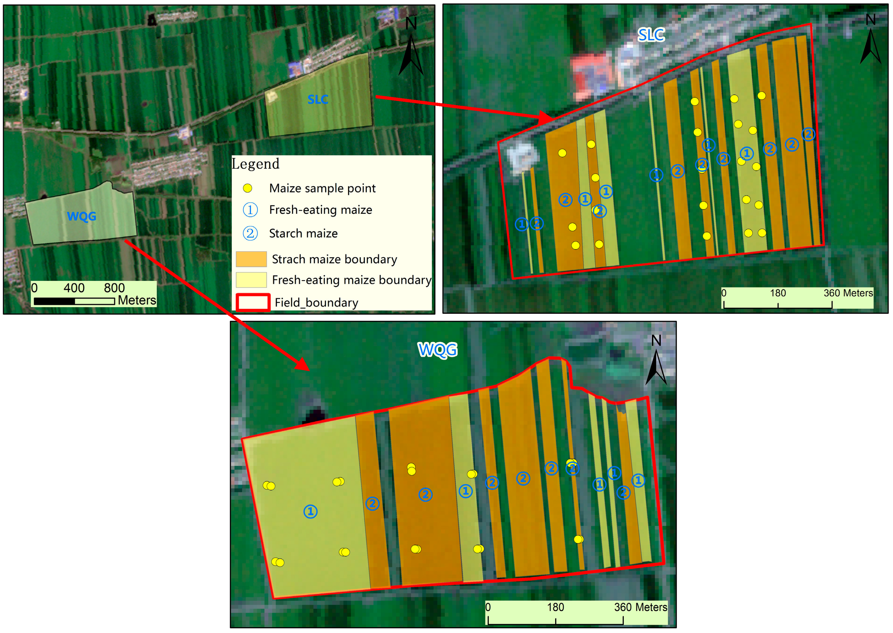
As depicted in Figure 1, this study was carried out on two black soil research experimental fields located in Hailun County, Heilongjiang Province, China. The county, located between 126°14′ E and 127°45′ E and 46°58′ N and 47°52′ N, experiences a temperate continental climate. The annual sunshine hours are 2315 h, the active accumulated temperature is 2200–2400 °C, the frost-free period is 117 days, and the annual average precipitation is 556 mm. From the northeast to the southwest, the topography transitions from low hills to high plains, river terraces, and floodplains, with gradual decreases in elevation. Hailun County is a key study area for black land research, with the reputation of being a high-starch maize hometown and also an important commodity grain base in China. In the 2021 growing season, the two intercropping fields of maize and soybean were planted with fresh-eating maize and starch maize, respectively, at the same sowing time. The first field (the central location point is 47.413° N, 126.747° E) named WQG has a total crop planting area of 50.3 ha, where maize accounts for about 75%. The second field (the central point is located at 47.427° N, 126.779° E) named SLC has a total planting area of 56 ha, where the planting area of maize accounts for 60%, greater than that of soybeans.
2.2. Multi-Spectral UAV Flight Campaign and Image Processing
The DJI Phantom4-M (P4M) UAV (Figure 2), equipped with a multi-spectral camera with six channels, including a visible channel and five multi-spectral sensor channels, was employed in this study to obtain multi-spectral UAV images. The descriptions of the multi-spectral camera bands are shown in Table 1. P4M was taken between 11 a.m. and 2 p.m. in clear and cloudless weather with a flight height setting of 190 m (the GSD, or ground sampling distance, is H/18.9 cm/pixel) and an 80% overlap in the heading direction and a 70% overlap in the side direction for each flight. Before the flight, the radiometric calibration board equipped with the camera was used for radiometric calibration. After the flight, the images were fed into the Pix4D mapper software (Version:4.4.10) for image mosaic. We obtained the image reflectance data for each field and then resampled the image data to a spatial resolution of 0.1 m. All of the collected UAV images were processed and analyzed using the ArcGIS software (Version:10.5).
2.3. Ground Data Collection
Maize in the two experimental fields with rich humus and nutrients was sown on 5 May 2021, with a row distance of 0.65 m and a plant distance of 0.15 m, respectively. The two fields had the same treatments, including the irrigation amount, fertilizer amount, and other management measures. The data of two field trials were collected at the three most important growth stages of maize, as shown in Figure 3 [52], which were on 12 July 2021, that is, the jointing stage of maize; 18 August 2021, that is, the milky maturity stage of maize; and 18 September 2021, that is, the maturity of maize. In this study, each sampling point covered a plot area of 1.3 m × 1.3 m. Twenty sampling points of maize were collected in the WQG field, including the LCC and LAI of the three maize growth stages and the GMC of maize at the maturity stage. We also collected 22 GMC sampling points of maize at the maturity stage in SLC. While collecting data from the ground, multi-spectral UAV images of each field were acquired simultaneously. The distribution of sampling points in the two fields is shown in Figure 4. Number ① represents fresh-eating maize planting strips, and number ② indicates starch maize planting strips. The exact coordinate information of each sample point was recorded by the Global Positioning System (GPS) with a centimeter-level differential positioning record.
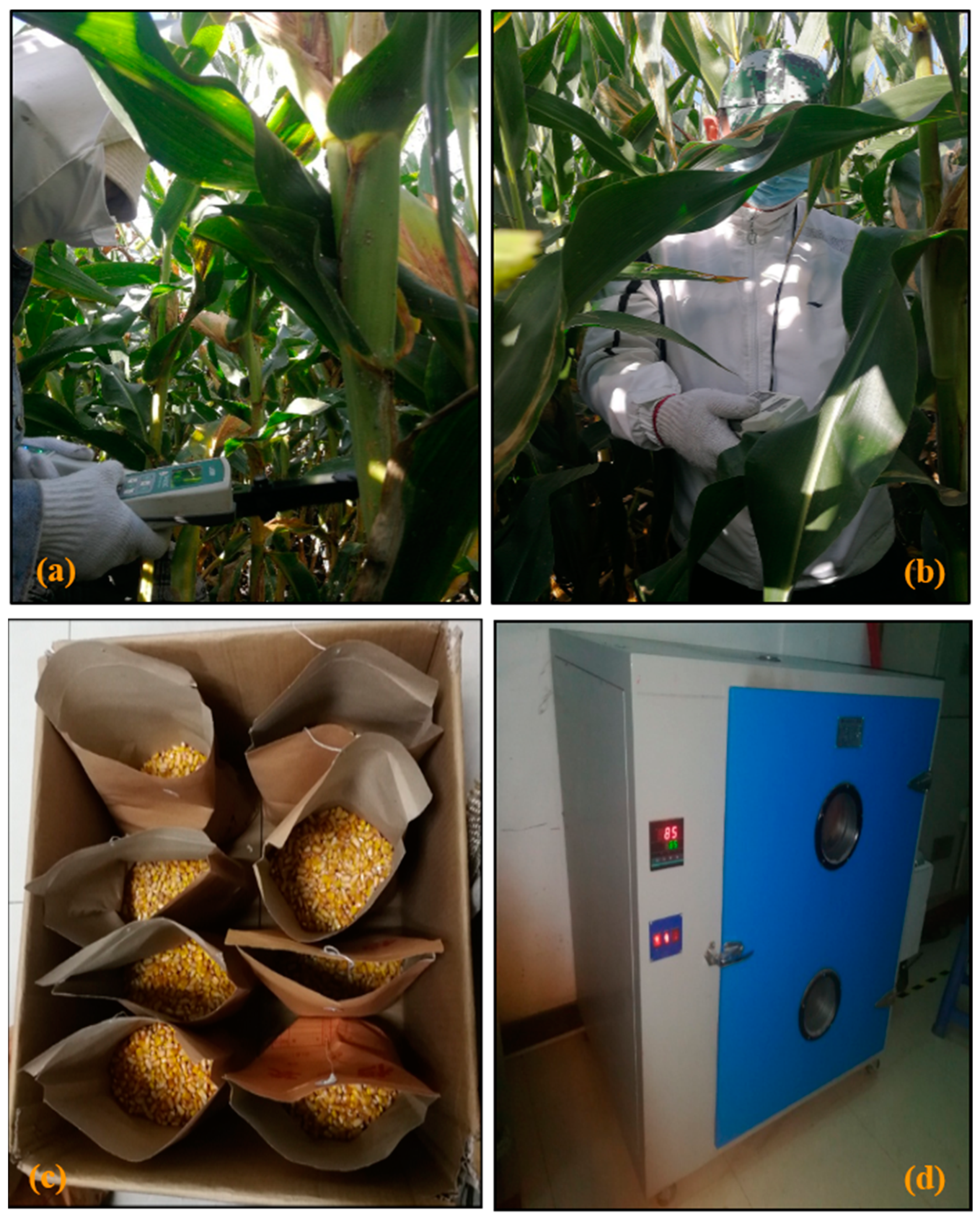
The LAI-2200c plant canopy analyzer (LI-COR, LNK, Lincoln, NE, USA) and the SPAD-502 chlorophyll meter (Riben, Konica Minolta, Tokyo, Japan) were used to quantify the LCC and LAI values, respectively. It was noticed that the values collected by SPAD are dimensionless and have a high correlation with LCC by an empirical correction function [53]. For obtaining LCC values at the same sample point, a total of 18 values of LCC were collected from the two maize plants that were closest to a sampling point. Each plant measured nine points distributed respectively in three leaves (each leaf having three values obtained in the top, middle, and bottom parts). The average of those measured SPAD values was recorded at this sampling point. For the LAI collection of each plant, a skylight and four target values near the root were needed for measuring to avoid the effects of direct sunlight. As a result, we also collected two LAI values from the same two maize plants, and the average of them was calculated and recorded.
All corncobs from the two plants at each sampling point were harvested and taken back to the lab on 18 September 2021, to measure the GMC of maize. To do this, the corncobs were first threshed, and the wet weight of the grains at each sampling location was measured using a high-precision balance. Subsequently, the wet grains were loaded in an oven set at 85° for a long time (over seven days) until they were fully dried (i.e., the weight did not change anymore). The dry weight of the grains was then measured, and the dry weight to wet weight ratio was calculated and employed as the ground true value of maize GMC. Figure 5 depicts the ground sampling data acquisition and the GMC measurement site, respectively. Table 2 displays the data collection at the various growth stages of maize in the experimental design from the study fields.
3. Methodology
In this paper, the assessment of maize maturity was achieved by an empirical model in land parcel WQG, in which the quantitative relationship between vegetation indices (VIs) obtained through UAV multi-spectral imagery, canopy chlorophyll content (CCC), and maize grain moisture content (GMC) at maturity was experimentally determined. Specifically, we first used the verified PROSAIL model to invert the maize CCC in the second land parcel (i.e., SLC). Next, we calculated various forms of VIs that are closely related to crop CCC, and then we constructed and evaluated empirical models for estimating maize GMC at maturity. Finally, a sensitivity analysis was conducted to examine how modifications to the PROSAIL model parameters and the corresponding variations of the CCC affected the reflectance of different UAV spectral bands. This was carried out to evaluate the rationality of establishing an empirical model to determine the optimal vegetation index.
3.1. PROSAIL Model for CCC Retrieval
Canopy chlorophyll content (CCC), defined as the product of leaf chlorophyll content (LCC) and leaf area index (LAI) (as shown in Equation (1) below) [54], is an important characteristic parameter for characterizing crop growth status in agricultural quantitative remote sensing (including inversion of crop maturity). The PROSAIL model was employed in our study to invert the maize CCC. It is an overall model derived by coupling PROPECT (leaf radiative transfer model) with SAIL (canopy structure model) [55,56,57,58], which mainly describes the optical characteristics of plant leaves in the spectral range of 400–2500 nm. The PROSPECT-5 model requires a series of leaf parameters, including leaf structure (N), chlorophyll a + b content (Cab), equivalent water thickness (Cw), dry matter content (Cm), carotenoid concentration (Car), and brown pigment (Cbp), while the 4-SAIL model necessitates the following parameters: leaf reflectance and transmittance (PROSPECT-5 output), leaf area index (LAI), hot spot parameter (hot), dry/wet soil factor (Psoil), soil brightness factor (Bsoil), average leaf inclination angle (ALIA) of a spherical leaf angle distribution function, sun zenith angle (θs), observer zenith angle (θv) and relative azimuth angle (φSV).
The maize biophysical parameters employed to feed the PROSAIL model were obtained from the literature except for Cab (i.e., LCC) and LAI [4,43,47,59,60]. Here, both Cab and LAI were acquired through field observations. The settings for each parameter range are shown in Table 3. For instance, the parameter N ranges between 1.2 and 2, Car varies between 0 and 12, and the values of Cab and LAI vary depending on the measured values at different growth stages of maize. The parameters Psoil (ranging between 0.05 and 0.4) and Bsoil (ranging between 0 and 1) represent soil moisture and soil brightness. The parameters θs, θv, and φSV are related to the time of flight and sensor information, which, in our case, have ranges between 0° and 45°, 0° and 30° and 0° and 180°, respectively.
The sensitivity analysis methodology proposed by [46] was performed to examine how various input parameters affect the output reflectance of the PROSAIL model. While the spectrum reflectance of the UAV images falls within a specific spectral range (as shown in Table 1), the simulated spectrum reflectance of the PROSAIL model is a smooth curve with an interval of 1 nm, indicating a significant scale influence between them. Therefore, the continuous spectral reflectance was transformed into the UAV multi-spectral reflectance in each band wavelength range based on the spectral response function (Equation (2)). We referenced [47], which utilized a cost function (the least squares error, LSE (Equation (3)) and a look-up table (LUT) approach to determine the best match between the simulated reflectance and the reflectance observed by the UAV images. Finally, the measured maize CCC data at the sixty ground points collected at different growth stages from WQG were used to verify the CCC inversion accuracy by the PROSAIL model.
The simulated UAV band reflectance () can be calculated as follows:
where and are the maximum and minimum wavelength ranges of each band of UAV (i.e., central wavelength adds and subtracts half of the band width for each UAV band), respectively; denotes the spectral response function; and represents the simulated reflectance derived from the PROSAIL model.
The least squares error (LSE) can be calculated as follows:
where and are, respectively, the true value and the estimate value, and represents the count of the sampling points.
During the sensitivity analysis process of selected VIs, we quantified the relative changes in the VIs value depending on maize CCC variations at maturity following Sun Y et al. (2019) [61] as follows:
where and are the vegetation index values corresponding to the maximum and minimum CCC of maize at maturity, respectively.
3.2. Calculation of VIs
In order to compare the estimation of the maize GMC at maturity by the CCC with a simple VI-based approach, several typical and commonly used VIs were calculated from multi-spectral UAV images, including NDVI, GNDVI, NDRE, RENDVI, and LCI (as shown in Table 4). These VIs have a good indication and sensitivity for assessing the growth status of crops, identifying different concentrations of chlorophyll in crops, and evaluating the degree of senescence. The VIs values at each ground sampling point were extracted from UAV images for further analysis.
3.3. Model Construction and Performance Assessment
To build empirical models between the CCC and maize GMC, as well as between the selected VIs and maize GMC at maturity, different regression models were tested, including exponential, linear, logarithmic, and power [4,22,47]. We first built the models only using the sampling points (ground-measured CCC and VIs) collected in WQG (as shown in Figure 4). The coefficient of determination (R2) was used to assess the performance of different models. Then, the established empirical models were cross-validated using the sampling points of SLC (as shown in Figure 4). The higher the goodness of the model, the closer the R2 is to 1. The calculation of R2 is shown in Equation (5), and its general range is from 0 to 1.
Furthermore, root mean square error (RMSE) and mean absolute error (MAE) were also used for assessing the statistical metrics of each cross-validation. The root mean square error (RMSE) reflects the deviation between the predicted value and the real value and the stability of the evaluation model. The smaller the RMSE value, the higher the accuracy of the model. The calculation method is shown in Equation (6):
MAE reflects the actual situation of the predicted value error. The smaller the value, the higher the accuracy of the model. The calculation method is shown in Equation (7):
In Equations (5)–(7), represents the predicted value, and respectively denotes the measured value and the average of the measured values; n is the total number of sampling points; and j is the serial number of each sampling point. Herein, the Origin software (Version: 2022.9.9.0.225) was used to perform the regression analysis, and Python 3.6 was used for graph generation.
4. Results
4.1. Results of Field Observations of LCC, LAI, and GMC
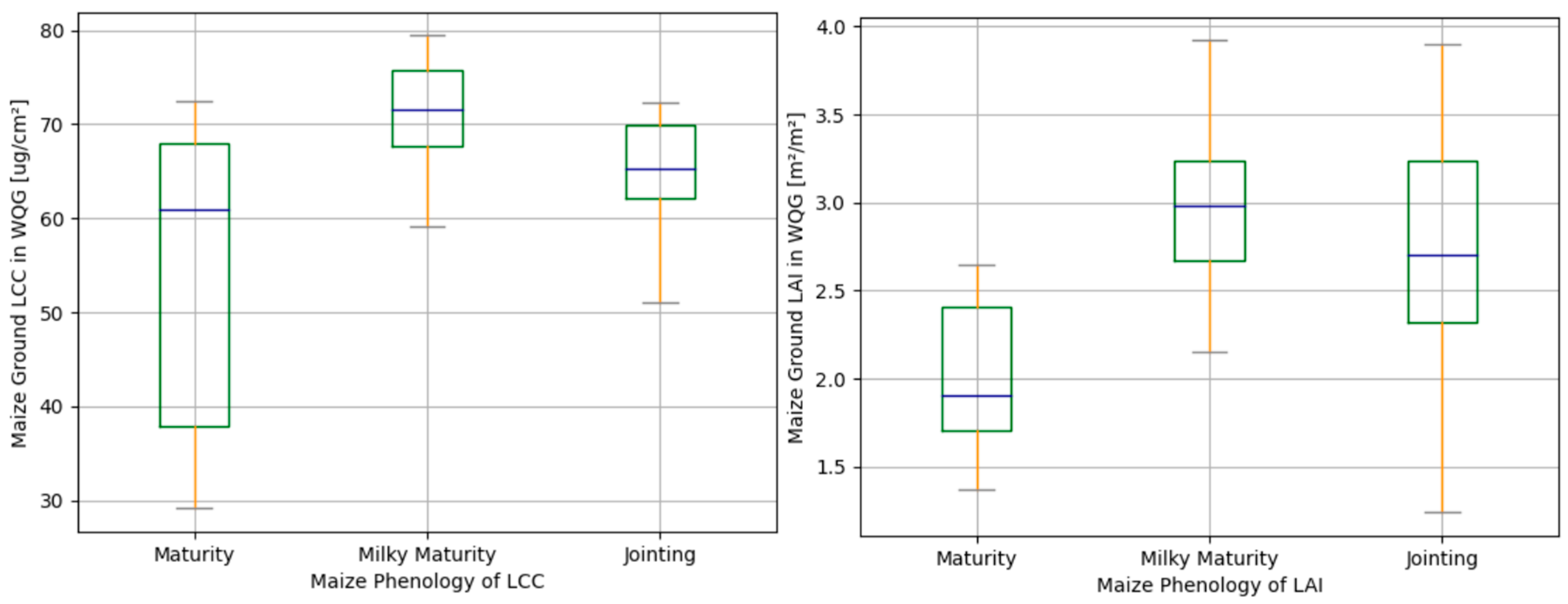
Figure 6 illustrates the ground-measured results of maize LCC and LAI at the WQG site. As can be seen, the LCC reached its peak at the milky maturity stage, followed by the jointing stage, and was lowest at the maturity stage. Similarly, the LAI was highest at the milky maturity stage, followed by the jointing stage, and reached its lowest during the maturity stage. That is, the changing trends of ground-measured maize LAI are consistent with those of maize LCC. The maize GMC values of the corresponding sample points at the maturity stage were also measured over both sites and demonstrated in Figure 7. It is clear that GMC values in both fields were relatively consistent, varying in a range between 0.37 and 0.46, with an average value of about 0.41.
4.2. Retrieval of Maize CCC from PROSAIL Inversion Model
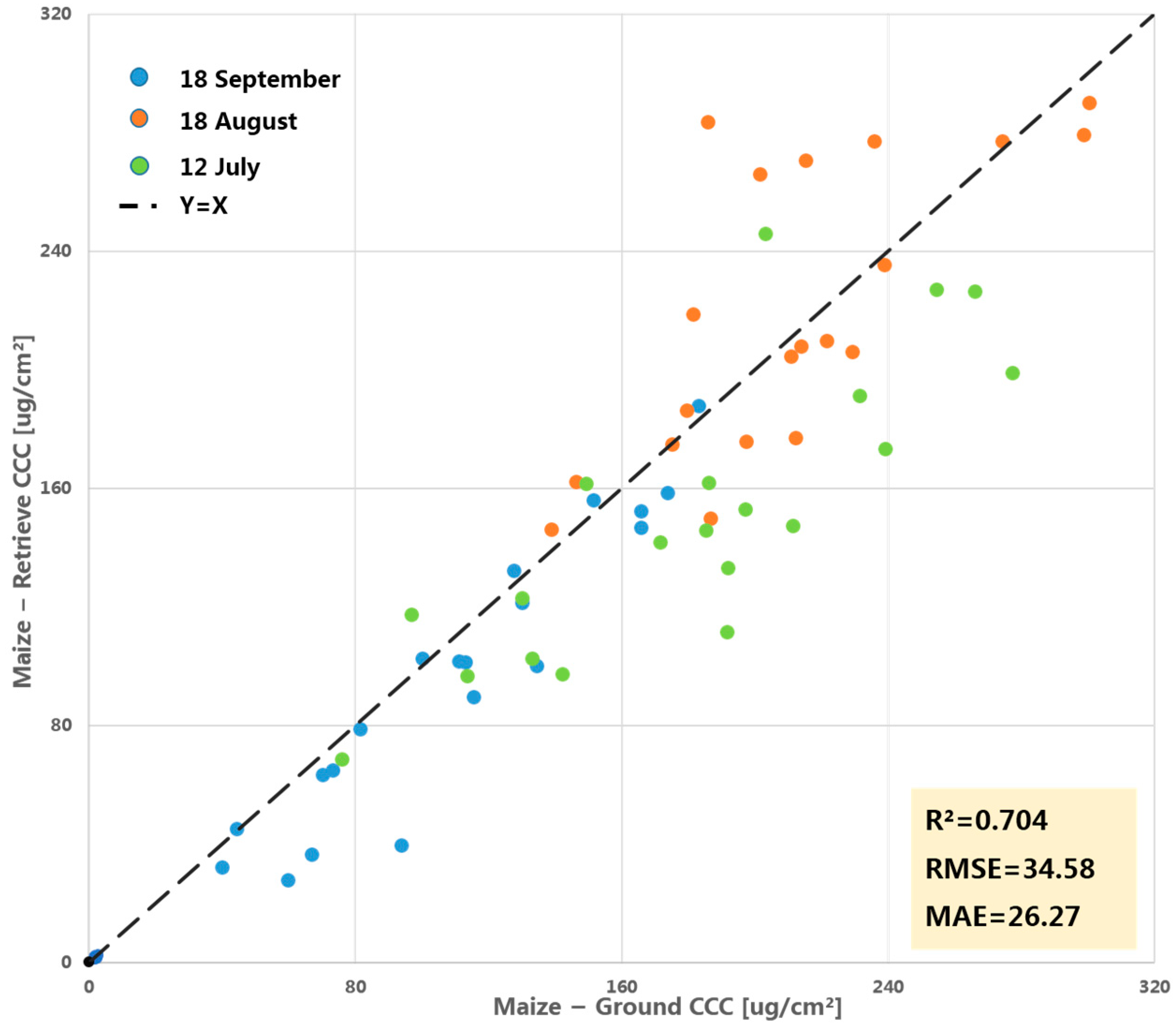
For each ground sample point, a total of 50,000 simulated spectral reflectance values were generated by the PROSAIL model. The best 10% simulated solutions that best matched (with the least square error) the corresponding ground-observed reflectance value were selected and averaged to retrieve the LCC and LAI values. Subsequently, the canopy chlorophyll content (CCC) for each ground sample point was calculated using Equation (1). The 60 ground-observed sampling points across different growth stages in WQG were used to validate the retrieved CCC results from the PROSAIL model. The validation results (Figure 8) showed an R2 value of 0.704 with a MAE of 26.27 μg/cm2 and a RMSE of 34.58 μg/cm2. This validated PROSAIL model was then used to retrieve the maize CCC values from another study site, SLC.
4.3. Correlation of Both CCC and VIs with GMC
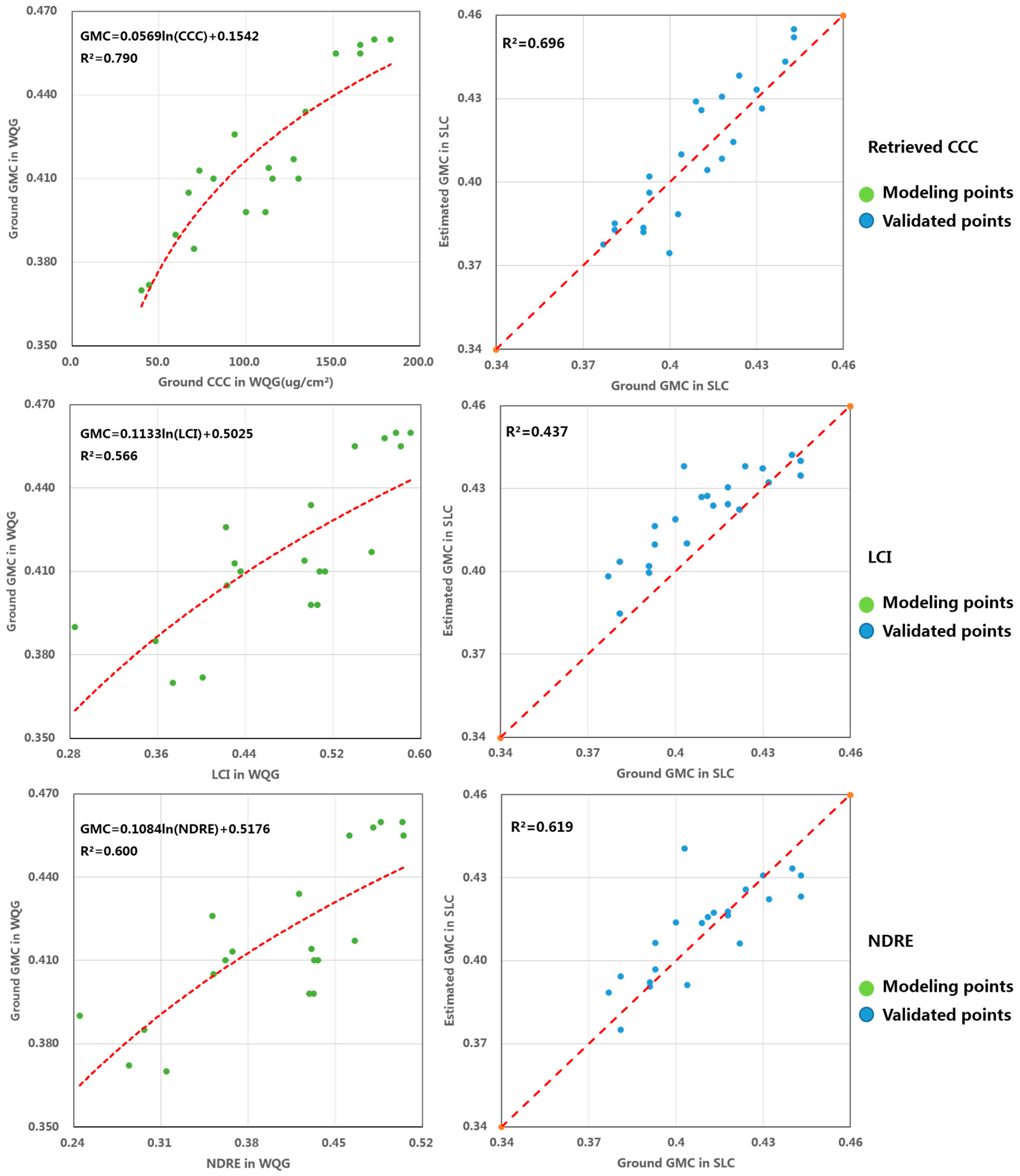
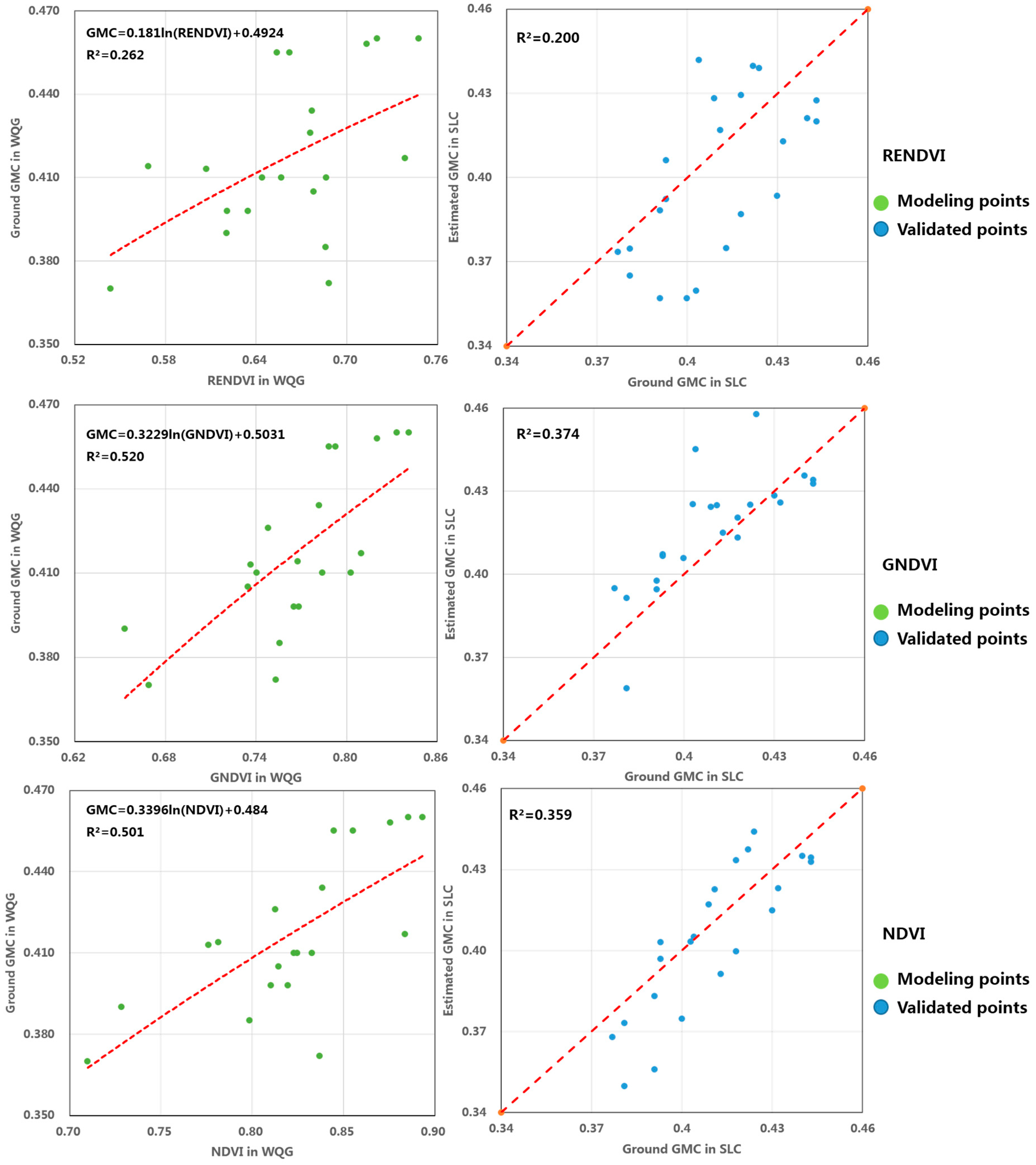
A correlation analysis of different chosen regression models was carried out to investigate the relationship between the measured CCC from the 20 ground sample points, the VIs calculated from UAV images, and the maize GMC at maturity in WQG. The best maize GMC retrieval model was further validated with the VIs and the retrieved CCC of 22 maize sampling points at maturity in SLC. Table 5 depicts the goodness of fitting between CCC, Vis, and maize GMC at maturity in different models. The p-values of different regression models for all parameters are <0.01, indicating that the established regression model has significant statistical significance. Among all the selected regression models, the logarithmic model achieved the optimal R2 values. Equations (8)–(13) in Table 6 show the optimal logarithmic regression model between maize GMC and CCC, LCI, NDRE, RENDVI, GNDVI, and NDVI from WQG and SLC. As shown in the table, CCC achieved the highest R2 values (0.79 and 0.696, respectively) in both WQG and SLC in comparison with all of the selected vegetation indices. Furthermore, amongst all vegetation indices, NDRE achieved the most accurate GMC retrieval results with R2 values greater than 0.6 in both sites, significantly greater than the LCI (0.566 and 0.437), the GNDVI (0.520 and 0.374), the NDVI (0.501 and 0.359), and the RENDVI (0.262 and 0.200). Figure 9 shows the scatterplots resulting from the cross-validation process, where maize GMC was estimated from the VIs and CCC logarithmic empirical models.
Figure 10 shows the inversion map of maize GMC at maturity based on the optimal vegetation index NDRE in both study sites. As we can see from the figure, the GMC of fresh-eating maize was commonly lower than that of starch maize at both sites. The distribution map of GMC pixel counts as shown in Figure 11 demonstrates that the maize GMC is primarily distributed between 0.370 and 0.435, accounting for more than 90% of the total number of maize pixels. The average values of maize GMC were 0.404 and 0.410 in WQG and SLC, respectively.
4.4. Parameter Sensitivities of the PROSAIL Model
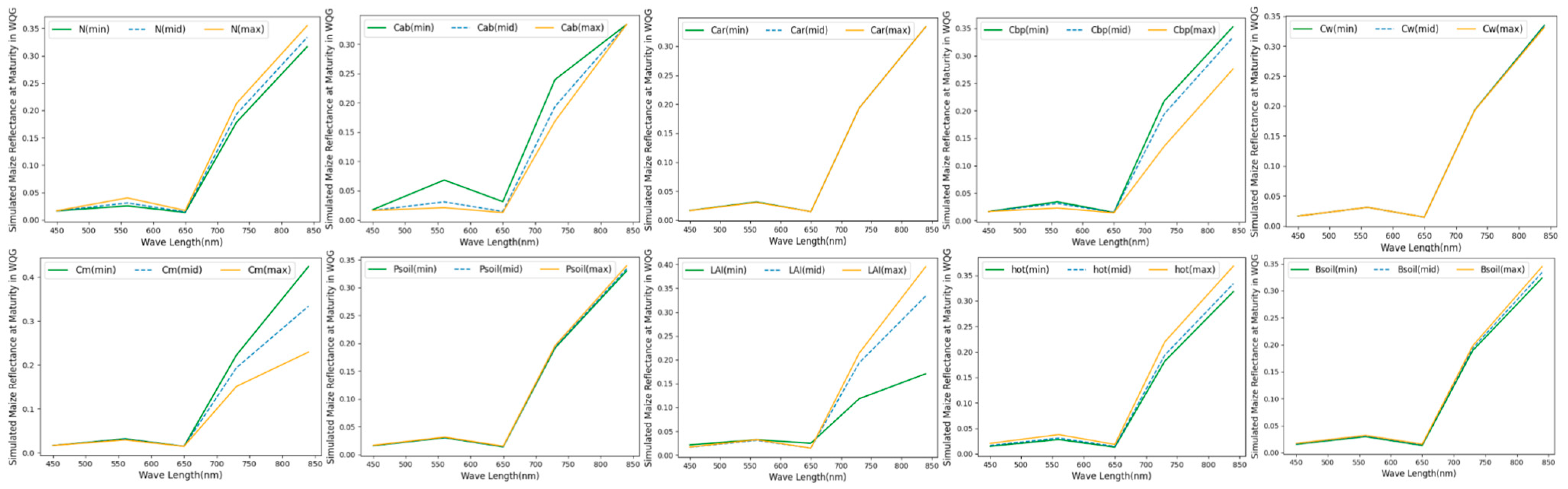
To assess the parameter sensitivity of the PROSAIL model, Figure 12 shows how changes in the parameters of the PROSAIL model affect maize spectral reflectance at the maturity stage over various wavelengths. As can be seen from the figure, the parameters Cab and LAI exerted the greatest influence on spectral reflectance. Specifically, Cab affected negatively the G (560 nm) and the RE (730 nm) bands, whereas LAI had a significant positive effect on the RE and the NIR (840 nm) bands. Similar to LAI, the parameters Cbp and Cm also had an impact on the RE and the NIR bands. The other parameters of PROSAIL, including N, Car, Cw, Psoil, Bsoil, and hot, had little effect on maize spectral reflectance.
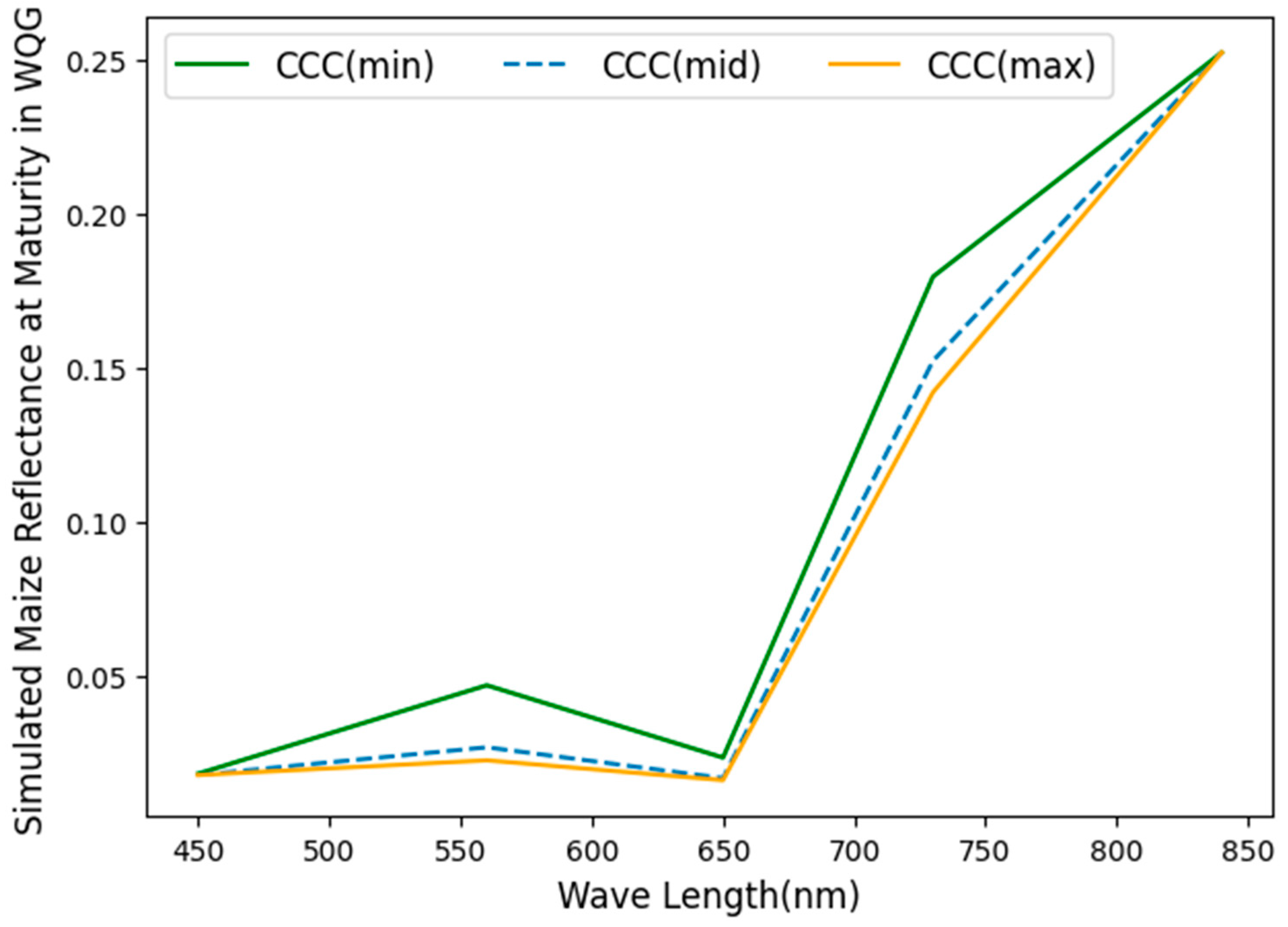
In order to further investigate the impact of maize CCC on spectral reflectance, we kept the parameters of the PROSAIL model fixed, except for Cab and LAI, and quantified how spectral reflectance responded to changes in maize CCC over different wavelengths (Figure 13). As shown in the figure, the RE (730 nm) band was most sensitive, followed by the G (560 nm) and R (650 nm) bands, and the NIR (840) and B (450) bands were insensitive to variations in maize CCC.
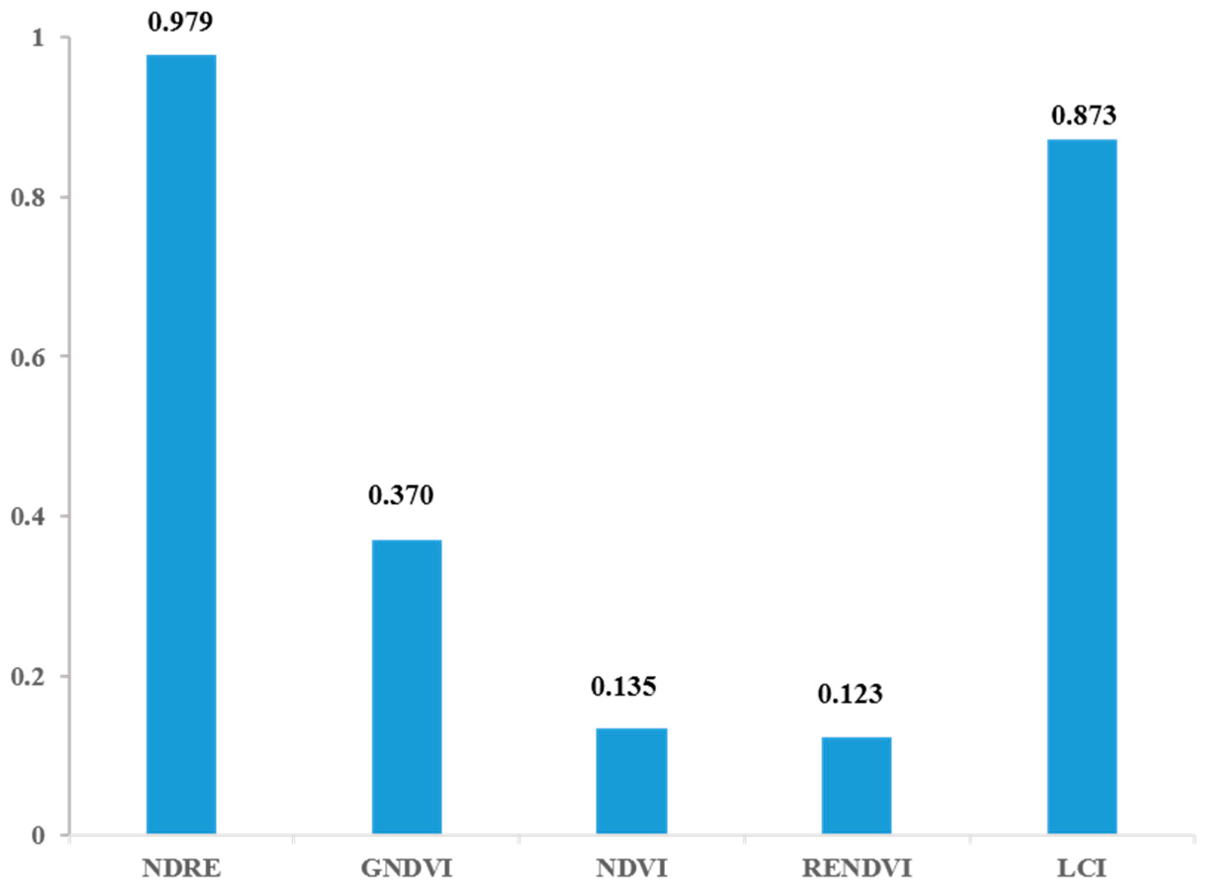
The sensitivity of the selected VIs to the variations in maize CCC at maturity was quantified (Equation (4)) and demonstrated in Figure 14. From the figure, it can be seen that the NDRE had the largest change, with a relative change value up to 0.979, followed by the LCI (0.873), GNDVI (0.370), NDVI (0.135), and the RENDVI, which achieved the smallest change (0.123). The figure also shows that the change in the value of vegetation indices (i.e., NDRE and LCI) with the RE (730 nm) band and the NIR (840 nm) band is obviously greater than that of others.
5. Discussion
5.1. Contributions of UAV in Maize Maturity Estimation
Due to its flexibility, convenience, and high spatial and temporal resolution, UAV remote sensing technology is emerging as a key tool for agricultural monitoring (e.g., yield estimation, pest monitoring, and plant identification). Previous studies demonstrated the effectiveness of UAV remote sensing for crop monitoring at small scales, such as fields, farms, and counties [22,23,24,47]. In this paper, this technology was used to observe and record the difference in crop growth conditions at a very fine scale, i.e., within and between fields, which was seldom involved in previous research. Maize from sowing to maturity is an overall growth process. The main factors affecting maize growth include environmental factors such as temperature and rainfall, terrain factors, crop varieties, planting conditions, et al. The selection of maize varieties affects their genetic traits, variety resistance, variety maturity, and grain quality [64,65]. Despite the identical environmental and planting conditions and the same planting time, the two maize varieties (fresh-eating maize and starch maize) show a relatively constant difference in maize maturity either within or between the two experimental fields (WQG and SLC): the GMC of fresh-eating maize was lower than that of starch maize with respect to maize maturity. Our proposed UAV remote sensing methodology was able to effectively capture such a maize maturity difference, demonstrating its usefulness for future precision management of maize.
5.2. The Theoretically Consistent VI-Based Estimation Model Based on CCC Validation
In our method, a theoretically consistent empirical model regarding the relationship between VIs (calculated from UAV remote sensing data) and the GMC of maize at maturity was built by providing enhanced CCC-based evidence. Canopy chlorophyll content (CCC), which is a multiplication of leaf chlorophyll content (LCC) and leaf area index (LAI), is a synthesized reflection of a crop’s green leaf status and canopy structure. Previous studies (e.g., Xu et al., 2019) [4] demonstrated a close relationship between the remote sensing-based CCC value and the GMC of maize at maturity. Specifically, when the CCC value decreases to a certain level, an obvious decrease in the GMC will occur. Such recognition was further proven by our field-based observations and related analysis. Furthermore, through the PROSAIL model’s inversion of CCC and the analysis of the model’s sensitivity, how changes in CCC concentration altered the reflectance of each UAV band was determined, and it was demonstrated that NDRE was the VI that was most impacted by the change in CCC.
5.3. Optimal Vegetation Index for Maize GMC Estimation
Our empirical models show that NDRE is the most robust vegetation index in the selected VIs for estimating GMC at the maturity stage of maize, although its inversion GMC accuracy is relatively lower than that of CCC, as illustrated by our results. It should be pointed out that the relatively higher accuracy of GMC inversion based on CCC (including the CCC inverted by a PROSAIL model) comes at the cost of the expensive and time-consuming acquisition of a large amount of field sampling data, thus significantly affecting the practicality of such a method. Furthermore, some uncertainty is also noticed for the CCC-based inversion approach due to the obvious variation of R2 values in the two plots in comparison with our VI-based approach. In contrast, NDRE is directly calculated by the RE band (730 nm) and NIR band (840 nm) of UAV-based remote sensing imagery, thereby saving the cost of field observation. The RE band, which is a narrower band located between the RED band and NIR band and has the largest change in the slope of a crop’s spectral reflectance curve, is very sensitive to changes in the chlorophyll content of vegetation, whereas soils and other terrestrial objects show smaller increases in reflectance [66,67,68]. Furthermore, the RE band and the NIR band are sensitive bands to LAI (as shown in Figure 11). The vegetation index, NDRE, therefore better represents the combination of chlorophyll content and canopy structure, i.e., CCC. This result is in agreement with previous findings. For example, according to Milas A et al. (2018) and Boiarskii B et al. (2018) [69,70], the NDRE vegetation index calculated based on multi-spectral UAV images was sensitive to and highly correlated with maize CCC when monitoring crop chlorophyll content; ref. [47] found that, in comparison with LAI, GNDVI, and NDVI, NDRE performed the best for predicting crop yield and biomass using high-resolution hyperspectral data.
5.4. Limitations and Future Work
Although the NDRE-based approach shows advantages in terms of efficiencies in the inversion of maize grain moisture content (GMC) at the mature stage, there is still a gap compared to the CCC-based approach regarding inversion accuracy. The NDRE and the maize GMC at maturity are moderately associated (as shown in Table 6, R2: WQG = 0.600, SLC = 0.619), which could explain more than 60% of the maize GMC at maturity with little variation in R2 values between the two fields, suggesting that the VI approach is not significantly influenced by the external environment. CCC explains 70–80% of maize GMC (as shown in Table 6, R2: WQG = 0.79, SLC = 0.696), showing a discrepancy of 10–20% between the VI-based inversion of maize GMC at maturity and the GMC retrieval using the CCC—a critical physiological parameter in the growing process of crops. Furthermore, the multi-spectral UAV images used in our research can be regarded as hyperspectral data after screening and extracting characteristic bands, which theoretically have the quantitative inversion capability equivalent to hyperspectral images [25]. Yet there is still a gap compared to hyperspectral images with a higher level of spectral details and spectral information for crop growth monitoring. Specifically, the spectral range of the UAV sensor channel used in our work is only 435–866 nm, making it incapable of covering band ranges longer than 866 nm, which might be useful for crop monitoring. For example, the short-wave infrared band (SWIR, 1100 nm–2500 nm) has an important indicator effect on the inversion of crop canopy water content. In the face of these challenges, our future studies will focus on more comprehensive crop spectral indicators and vegetation indices to establish a more reliable remote sensing inversion method for crop dynamic growth monitoring and maturity analysis.
6. Conclusions
Timely, efficient, and accurate monitoring of crop maturity is vital for crop harvest management. Based on in situ sampling data, the potential of incorporating VI-based model inversion with a CCC-based model for estimating maize GMC at maturity was investigated. We found that the GMC at maturity was closely related to the variety of maize, and the PROSAIL inversion model was able to retrieve maize CCC with a reasonable R2 value, thus providing strong support for maize maturity analysis. Furthermore, the NDRE performed better (more accurate and stable) in comparison with other selected vegetation indices for maize GMC estimation at maturity. Nevertheless, we demonstrated that the UAV VI-based method has the capability of monitoring maize GMC accurately and flexibly over large areas. Future studies can explore the possibility of generalizing our established method to other regions and for other crops.
Author Contributions
Conceptualization, Z.L., X.D. and S.Z.; funding acquisition, H.L.; methodology, Z.L. and S.Z.; resources, H.L.; software, Z.L.; validation, Z.L.; writing—original draft, Z.L.; writing—review and editing, H.L., X.D., X.C., H.C. and S.Z. All authors have read and agreed to the published version of the manuscript.
Funding
This work was funded absolutely by the Special Project of Strategic Leading Science and Technology of the Chinese Academy of Sciences (No. XDA28070503).
Data Availability Statement
Data will be made available upon reasonable request.
Conflicts of Interest
The authors declare that they have no known competing financial interests or personal relationships that could have appeared to influence the work reported in this paper.
References
- FAO. FAOSTAT-Agriculture Database. 2021. Available online: http://www.fao.org/statistics/zh/ (accessed on 9 May 2022).
- Meng, J.H.; Dong, T.; Zhang, M.; You, X.; Wu, B. Predicting optimal soybean harvesting dates with satellite data. In Precision Agriculture’13; Wageningen Academic Publishers: Wageningen, The Netherlands, 2013; pp. 209–215. [Google Scholar]
- Meng, J.; Xu, J.; You, X. Optimizing soybean harvest date using HJ-1 satellite imagery. Precis. Agric. 2015, 16, 164–179. [Google Scholar] [CrossRef]
- Xu, J.; Meng, J.; Quackenbush, L.J. Use of remote sensing to predict the optimal harvest date of corn. Field Crops Res. 2019, 236, 1–13. [Google Scholar] [CrossRef]
- Wang, Z.; Guo, T.; Wu, X.; Zheng, W.; Liu, Z.; Zhang, M. Study on the influence of harvest time on the oil and yield of different mature period high-oil soybean. Chin. Agric. Sci. Bull. 2009, 25, 74–77. [Google Scholar]
- Liu, Z.; Wan, W.; Huang, J.; Han, Y.W.; Wang, J.Y. Progress on key parameters inversion of crop growth based on unmanned aerial vehicle remote sensing. Trans. Chin. Soc. Agric. Eng. (Trans. CSAE) 2018, 34, 60–71. [Google Scholar]
- Jihua, M.; Bingfang, W. The Feasibility Analysis on Satellite Data based Crop Mature Data Prediction. Remote Sens. Technol. Appl. 2013, 28, 165–173. [Google Scholar]
- Pordesimo, L.O.; Sokhansanj, S.; Edens, W.C. Moisture and yield of corn stover fractions before and after grain maturity. Trans. ASAE 2004, 47, 1597. [Google Scholar] [CrossRef]
- Tolera, A.; Sundstøl, F.; Said, A.N. The effect of stage of maturity on yield and quality of maize grain and stover. Anim. Feed. Sci. Technol. 1998, 75, 157–168. [Google Scholar] [CrossRef]
- Boogaard, H.L. User’s Guide for the WOFOST 7.1 Crop Growth Simulation Model and WOFOST Control Center 1.5 Technical Document 52 DLO Vinand Staring Centre; Soil and Water Research: São Paulo, Brazil, 1998. [Google Scholar]
- Brisson, N.; Mary, B.; Ripoche, D.; Jeuffroy, M.H.; Ruget, F.; Nicoullaud, B.; Gate, P.; Devienne-Barret, F.; Antonioletti, R.; Durr, C.; et al. STICS: A generic model for the simulation of crops and their water and nitrogen balances. I. Theory and parameterization applied to wheat and corn. Agronomie 1998, 18, 311–346. [Google Scholar] [CrossRef]
- Jones, J.W.; White, J.; Boote, K.; Hoogenboom, G.; Porter, C.H. Phenology Module in DSSAT v. 4.0: Documentation and Source Code Listing; University of Florida: Gainesville, FL, USA, 2000. [Google Scholar]
- Ailian, C.H.E.N.; Sijian, Z.H.A.O.; Yuxia, Z.H.U.; Wei, S.U.N. Application Scenarios and Research Progress of Remote Sensing Technology in Plant Income Insurance. Smart Agric. 2022, 4, 57. [Google Scholar]
- Pan, H.; Chen, Z.; de Wit, A.; Ren, J. Joint assimilation of leaf area index and soil moisture from sentinel-1 and sentinel-2 data into the WOFOST model for winter wheat yield estimation. Sensors 2019, 19, 3161. [Google Scholar] [CrossRef]
- Weiss, M.; Jacob, F.; Duveiller, G. Remote sensing for agricultural applications: A meta-review. Remote Sens. Environ. 2020, 236, 111402. [Google Scholar] [CrossRef]
- Han-ya, I.; Ishii, K.; Noguchi, N. Acquisition and analysis of wheat growth information using satellite and aerial vehicle imageries. In Proceedings of the 3rd Asian Conference on Precision Agriculture, Beijing, China, 14–17 October 2009. [Google Scholar]
- Alonzo, M.; Bookhagen, B.; McFadden, J.P.; Sun, A.; Roberts, D.A. Mapping urbanforest leaf area index with airborne LiDAR using penetration metrics and allometry. Remote Sens. Environ. 2015, 162, 141–153. [Google Scholar] [CrossRef]
- Yu, N.; Li, L.; Schmitz, N.; Tian, L.F.; Greenberg, J.A.; Diers, B.W. Development of methods to improve soybean yield estimation and predict plant maturity with an unmanned aerial vehicle based platform. Remote Sens. Environ. 2016, 187, 91–101. [Google Scholar] [CrossRef]
- Zhang, L.; Zhang, H.; Niu, Y.; Han, W. Mapping maize water stress based on UAV multispectral remote sensing. Remote Sens. 2019, 11, 605. [Google Scholar] [CrossRef]
- Xiang, H.; Tian, L. Development of a low-cost agricultural remote sensing system based on an autonomous unmanned aerial vehicle (UAV). Biosyst. Eng. 2011, 108, 174–190. [Google Scholar] [CrossRef]
- Zhang, C.; Kovacs, J.M. The application of small unmanned aerial systems for precision agriculture: A review. Precis. Agric. 2012, 13, 693–712. [Google Scholar] [CrossRef]
- Qi, H.; Wu, Z.; Zhang, L.; Li, J.; Zhou, J.; Jun, Z.; Zhu, B. Monitoring of peanut leaves chlorophyll content based on drone-based multispectral image feature extraction. Comput. Electron. Agric. 2021, 187, 106292. [Google Scholar] [CrossRef]
- Qiao, L.; Tang, W.; Gao, D.; Zhao, R.; An, L.; Li, M.; Sun, H.; Song, D. UAV-based chlorophyll content estimation by evaluating vegetation index responses under different crop coverages. Comput. Electron. Agric. 2022, 196, 106775. [Google Scholar] [CrossRef]
- Su, W.; Wang, W.; Liu, Z.; Zhang, M.; Bian, H.; Cui, Y.; Huang, J. Determining the retrieving parameters of corn canopy LAI and chlorophyll content computed using UAV image. Trans. Chin. Soc. Agric. Eng. (Trans. CSAE) 2020, 36, 58–65. [Google Scholar]
- Liu, T.; Zhang, H.; Wang, Z.Y.; He, C.; Zhang, Q.G.; Jiao, Y.Z. Estimation of the leaf index and chlorophyll content of wheat using UAV multi-spectrum images. Trans. Chin. Soc. Agric. Eng. (Trans. CSAE) 2021, 37, 65–72. [Google Scholar]
- Moeinizade, S.; Pham, H.; Han, Y.; Dobbels, A.; Hu, G. An applied deep learning approach for estimating soybean relative maturity from UAV imagery to aid plant breeding decisions. Mach. Learn. Appl. 2022, 7, 100233. [Google Scholar] [CrossRef]
- Sheng-hui, Y.; Yong-jun, Z.; Xing-xing, L.; Tian-gang, Z.; Xiao-shuan, Z.; Li-ming, X. Cabernet Gernischt Maturity Dtermination Based on Near-Ground Multispectral Figures by using UAVs. Spectrosc. Spectr. Anal. 2021, 41, 3220–3226. [Google Scholar]
- Caballero, D.; Calvini, R.; Amigo, J.M. Hyperspectral imaging in crop fields: Precision agriculture. In Data Handling in Science and Technology; Elsevier: Amsterdam, The Netherlands, 2020; Volume 32, pp. 453–473. [Google Scholar]
- Croft, H.; Chen, J.M.; Zhang, Y.; Simic, A. Modelling leaf chlorophyll content in broadleaf and needle leaf canopies from ground, CASI, Landsat TM 5 and MERIS reflectance data. Remote Sens. Environ. 2013, 133, 128–140. [Google Scholar] [CrossRef]
- Clevers, J.G.; Kooistra, L.; Schaepman, M.E. Estimating canopy water content using hyperspectral remote sensing data. Int. J. Appl. Earth Obs. Geoinf. 2010, 12, 119–125. [Google Scholar] [CrossRef]
- Danner, M.; Berger, K.; Wocher, M.; Mauser, W.; Hank, T. Fitted PROSAIL parameterization of leaf inclinations, water content and brown pigment content for winter wheat and maize canopies. Remote Sens. 2019, 11, 1150. [Google Scholar] [CrossRef]
- Delloye, C.; Weiss, M.; Defourny, P. Retrieval of the canopy chlorophyll content from Sentinel-2 spectral bands to estimate nitrogen uptake in intensive winter wheat cropping systems. Remote Sens. Environ. 2018, 216, 245–261. [Google Scholar] [CrossRef]
- Duan, S.B.; Li, Z.L.; Wu, H.; Tang, B.H.; Ma, L.; Zhao, E.; Li, C. Inversion of the PROSAIL model to estimate leaf area index of maize, potato, and sunflower fields from unmanned aerial vehicle hyperspectral data. Int. J. Appl. Earth Obs. Geoinf. 2014, 26, 12–20. [Google Scholar] [CrossRef]
- Houborg, R.; Anderson, M.; Daughtry, C. Utility of an image-based canopy reflectance modeling tool for remote estimation of LAI and leaf chlorophyll content at the field scale. Remote Sens. Environ. 2009, 113, 259–274. [Google Scholar] [CrossRef]
- Huang, J.; Gómez-Dans, J.L.; Huang, H.; Ma, H.; Wu, Q.; Lewis, P.E.; Liang, S.; Chen, Z.; Xue, J.H.; Wu, Y.; et al. Assimilation of remote sensing into crop growth models: Current status and perspectives. Agric. For. Meteorol. 2019, 276, 107609. [Google Scholar] [CrossRef]
- Rouse, J.W., Jr.; Haas, R.H.; Deering, D.W.; Schell, J.A.; Harlan, J.C. Monitoring the Vernal Advancement and Retrogradation (Green Wave Effect) of Natural Vegetation; NASA: Greenbelt, MD, USA, 1974.
- Gitelson, A.A.; Kaufman, Y.J.; Merzlyak, M.N. Use of a green channel in remote sensing of global vegetation from EOS-MODIS. Remote Sens. Environ. 1996, 58, 289–298. [Google Scholar] [CrossRef]
- Hatfield, J.L.; Gitelson, A.A.; Schepers, J.S.; Walthall, C.L. Application of spectral remote sensing for agronomic decisions. Agron. J. 2008, 100, S-117–S-131. [Google Scholar] [CrossRef]
- Shuang, L.; Hai-ye, Y.; Jun-he, Z.; Hai-gen, Z.; Li-juan, K.; Lei, Z.; Jing-min, D.; Yuan-yuan, S. Study on Inversion Model of Chlorophyll Content in Soybean Leaf Based on Optimal Spectral Indices. Spectrosc. Spectr. Anal. 2021, 41, 1912. [Google Scholar]
- Donnelly, A.; Yu, R.; Rehberg, C.; Meyer, G.; Young, E.B. Leaf chlorophyll estimates of temperate deciduous shrubs during autumn senescence using a SPAD-502 meter and calibration with extracted chlorophyll. Ann. For. Sci. 2020, 77, 1–12. [Google Scholar] [CrossRef]
- Mao, Z.H.; Deng, L.; Duan, F.Z.; Li, X.J.; Qiao, D.Y. Angle effects of vegetation indices and the influence on prediction of SPAD values in soybean and maize. Int. J. Appl. Earth Obs. Geoinf. 2020, 93, 102198. [Google Scholar] [CrossRef]
- Atzberger, C.; Darvishzadeh, R.; Immitzer, M.; Schlerf, M.; Skidmore, A.; Le Maire, G. Comparative analysis of different retrieval methods for mapping grassland leaf area index using airborne imaging spectroscopy. Int. J. Appl. Earth Obs. Geoinf. 2015, 43, 19–31. [Google Scholar] [CrossRef]
- Bandaru, V.; Yaramasu, R.; Jones, C.; Izaurralde, R.C.; Reddy, A.; Sedano, F.; Daughtry, C.S.; Becker-Reshef, I.; Justice, C. Geo-CropSim: A Geo-spatial crop simulation modeling framework for regional scale crop yield and water use assessment. ISPRS J. Photogramm. Remote Sens. 2022, 183, 34–53. [Google Scholar] [CrossRef]
- Darvishzadeh, R.; Skidmore, A.; Schlerf, M.; Atzberger, C. Inversion of a radiative transfer model for estimating vegetation LAI and chlorophyll in a heterogeneous grassland. Remote Sens. Environ. 2008, 112, 2592–2604. [Google Scholar] [CrossRef]
- Jay, S.; Maupas, F.; Bendoula, R.; Gorretta, N. Retrieving LAI, chlorophyll and nitrogen contents in sugar beet crops from multi-angular optical remote sensing: Comparison of vegetation indices and PROSAIL inversion for field phenotyping. Field Crops Res. 2017, 210, 33–46. [Google Scholar] [CrossRef]
- Jiang, H.Y.; Chai, L.N.; Jia, K.; Liu, J.; Yang, S.Q.; Zheng, J. Estimation of water content for short vegetation based on PROSAIL model and vegetation water indices. Natl. Remote Sens. Bull. 2021, 25, 1025–1036. [Google Scholar] [CrossRef]
- Kayad, A.; Rodrigues Jr, F.A.; Naranjo, S.; Sozzi, M.; Pirotti, F.; Marinello, F.; Schulthess, U.; Defourny, P.; Gerard, B.; Weiss, M. Radiative transfer model inversion using high-resolution hyperspectral airborne imagery–Retrieving maize LAI to access biomass and grain yield. Field Crops Res. 2022, 282, 108449. [Google Scholar] [CrossRef]
- Punalekar, S.M.; Verhoef, A.; Quaife, T.L.; Humphries, D.; Bermingham, L.; Reynolds, C.K. Application of Sentinel-2A data for pasture biomass monitoring using a physically based radiative transfer model. Remote Sens. Environ. 2018, 218, 207–220. [Google Scholar] [CrossRef]
- Richter, K.; Atzberger, C.; Vuolo, F.; D’Urso, G. Evaluation of sentinel-2 spectral sampling for radiative transfer model based LAI estimation of wheat, sugar beet, and maize. IEEE J. Sel. Top. Appl. Earth Obs. Remote Sens. 2010, 4, 458–464. [Google Scholar] [CrossRef]
- Sehgal, V.K.; Chakraborty, D.; Sahoo, R.N. Inversion of radiative transfer model for retrieval of wheat biophysical parameters from broadband reflectance measurements. Inf. Process. Agric. 2016, 3, 107–118. [Google Scholar] [CrossRef]
- Wei, S.; Jia-yu, W.; Xin-sheng, W.; Zi-xuan, X.; Ying, Z.; Wan-cheng, T.; Tian, J. Retrieving Corn Canopy Leaf Area Index Based on Sentinel-2 Image and PROSAIL Model Parameter Calibration. Spectrosc. Spectr. Anal. 2021, 41, 1891–1897. [Google Scholar]
- Zhang, H.; Kang, J.; Xu, X.; Zhang, L. Accessing the temporal and spectral features in crop type mapping using multi-temporal Sentinel-2 imagery: A case study of Yi’an County, Heilongjiang province, China. Comput. Electron. Agric. 2020, 176, 105618. [Google Scholar] [CrossRef]
- Markwell, J.; Osterman, J.C.; Mitchell, J.L. Calibration of the Minolta SPAD-502 leaf chlorophyll meter. Photosynth. Res. 1995, 46, 467–472. [Google Scholar] [CrossRef]
- Chakhvashvili, E.; Siegmann, B.; Muller, O.; Verrelst, J.; Bendig, J.; Kraska, T.; Rascher, U. Retrieval of Crop Variables from Proximal Multispectral UAV Image Data Using PROSAIL in Maize Canopy. Remote Sens. 2022, 14, 1247. [Google Scholar] [CrossRef]
- Feret, J.B.; François, C.; Asner, G.P.; Gitelson, A.A.; Martin, R.E.; Bidel, L.P.; Ustin, S.L.; Le Maire, G.; Jacquemoud, S. PROSPECT-4 and 5: Advances in the leaf optical properties model separating photosynthetic pigments. Remote Sens. Environ. 2008, 112, 3030–3043. [Google Scholar] [CrossRef]
- Jacquemoud, S.; Baret, F. PROSPECT: A model of leaf optical properties spectra. Remote Sens. Environ. 1990, 34, 75–91. [Google Scholar] [CrossRef]
- Jacquemoud, S.; Verhoef, W.; Baret, F.; Bacour, C.; Zarco-Tejada, P.J.; Asner, G.P.; François, C.; Ustin, S.L. PROSPECT+ SAIL models: A review of use for vegetation characterization. Remote Sens. Environ. 2009, 113, S56–S66. [Google Scholar] [CrossRef]
- Verhoef, W. Light scattering by leaf layers with application to canopy reflectance modeling: The SAIL model. Remote Sens. Environ. 1984, 16, 125–141. [Google Scholar] [CrossRef]
- Gutman, G.; Skakun, S.; Gitelson, A. Revisiting the use of red and near-infrared reflectances in vegetation studies and numerical climate models. Sci. Remote Sens. 2021, 4, 100025. [Google Scholar] [CrossRef]
- Zhang, M.Z.; Su, W.; Zhu, D.H. Retriecal of LAI and LCC in Summer Corn Canopy Based on the PROSAIL Model Using an Improved Inversion Strategy. Geogr. Geo-Inf. Sci. 2019, 35, 28–33. [Google Scholar]
- Sun, Y.; Qin, Q.; Ren, H.; Zhang, T.; Chen, S. Red-edge band vegetation indices for leaf area index estimation from Sentinel-2/MSI imagery. IEEE Trans. Geosci. Remote Sens. 2019, 58, 826–840. [Google Scholar] [CrossRef]
- Elsayed, S.; Rischbeck, P.; Schmidhalter, U. Comparing the performance of active and passive reflectance sensors to assess the normalized relative canopy temperature and grain yield of drought-stressed barley cultivars. Field Crops Res. 2015, 177, 148–160. [Google Scholar] [CrossRef]
- Kaur, R.; Singh, B.; Singh, M.; Thind, S.K. Hyperspectral indices, correlation and regression models for estimating growth parameters of wheat genotypes. J. Indian Soc. Remote Sens. 2015, 43, 551–558. [Google Scholar] [CrossRef]
- Chimonyo, V.G.P.; Mutengwa, C.S.; Chiduza, C.; Tandzi, L.N. Participatory variety selection of maize genotypes in the Eastern Cape Province of South Africa. S. Afr. J. Agric. Ext. 2019, 47, 103–117. [Google Scholar] [CrossRef]
- Louette, D.; Smale, M. Farmers’ seed selection practices and traditional maize varieties in Cuzalapa, Mexico. Euphytica 2000, 113, 25–41. [Google Scholar] [CrossRef]
- Matsushita, B.; Yang, W.; Chen, J.; Onda, Y.; Qiu, G. Sensitivity of the enhanced vegetation index (EVI) and normalized difference vegetation index (NDVI) to topographic effects: A case study in high-density cypress forest. Sensors 2007, 7, 2636–2651. [Google Scholar] [CrossRef]
- Corti, M.; Cavalli, D.; Cabassi, G.; Gallina, P.M.; Bechini, L. Does remote and proximal optical sensing successfully estimate maize variables? A review. Eur. J. Agron. 2018, 99, 37–50. [Google Scholar] [CrossRef]
- Scotford, I.M.; Miller, P.C.H. Applications of spectral reflectance techniques in northern European cereal production: A review. Biosyst. Eng. 2005, 90, 235–250. [Google Scholar] [CrossRef]
- Simic Milas, A.; Romanko, M.; Reil, P.; Abeysinghe, T.; Marambe, A. The importance of leaf area index in mapping chlorophyll content of corn under different agricultural treatments using UAV images. Int. J. Remote Sens. 2018, 39, 5415–5431. [Google Scholar] [CrossRef]
- Boiarskii, B.; Hasegawa, H. Comparison of NDVI and NDRE indices to detect differences in vegetation and chlorophyll content. J. Mech. Contin. Math. Sci. 2019, 4, 20–29. [Google Scholar] [CrossRef]
Figure 1.
Location of the two fields (WQG and SLC) in Hailun County, Heilongjiang Province, China.

Figure 2.
Photos of the DJI P4M-UAV and the multi-spectral camera.

Figure 3.
Phenological calendars of maize in the study area.

Figure 4.
Locations of the sampling points in the two fields: WQG and SLC.

Figure 5.
Photos of ground data collection. (a) LAI measurement, (b) LCC measurement, and (c,d) maize drying.
Figure 5.
Photos of ground data collection. (a) LAI measurement, (b) LCC measurement, and (c,d) maize drying.

Figure 6.
Boxplot of ground maize LCC and LAI measurements at each key crop phenology for WQG.

Figure 7.
Boxplot of ground maize GMC at maturity in each field.

Figure 8.
Cross-validation between WQG-maize ground CCC and PROSAIL-retrieved CCC at different maize phenology.
Figure 8.
Cross-validation between WQG-maize ground CCC and PROSAIL-retrieved CCC at different maize phenology.

Figure 9.
Ground maize GMC against estimated maize GMC achieved using CCC and VIs empirical models in WQG and SLC (The red line on the left represents the fitted curve, and the red line on the right represents the 1:1 line.).
Figure 9.
Ground maize GMC against estimated maize GMC achieved using CCC and VIs empirical models in WQG and SLC (The red line on the left represents the fitted curve, and the red line on the right represents the 1:1 line.).


Figure 10.
Maps of maize GMC at maturity generated with the NDRE vegetation index in the two study sites.
Figure 10.
Maps of maize GMC at maturity generated with the NDRE vegetation index in the two study sites.

Figure 11.
Distribution of pixel counts for maize GMC at maturity in each study site.

Figure 12.
PROSAIL model spectral response sensitivity analysis curve under different input parameter values of maize at maturity.
Figure 12.
PROSAIL model spectral response sensitivity analysis curve under different input parameter values of maize at maturity.

Figure 13.
The spectral response sensitivity analysis curve under different maize CCC values at maturity.
Figure 13.
The spectral response sensitivity analysis curve under different maize CCC values at maturity.

Figure 14.
Relative changes in vegetation indices (ΔVI) under different maize CCC values at maturity.
Figure 14.
Relative changes in vegetation indices (ΔVI) under different maize CCC values at maturity.


Table 1.
Descriptions of the DJI P4M-UAV multi-spectral camera bands.
| Band Name | Center Wavelength/nm | Band Width/nm | File Suffix Name |
|---|---|---|---|
| Blue (B) | 450 | 32 | .tif |
| Green (G) | 560 | 32 | .tif |
| Red (R) | 650 | 32 | .tif |
| Red Edge (RE) | 730 | 32 | .tif |
| Near IR (NIR) | 840 | 52 | .tif |
Table 2.
Collection data during different growth stages of maize.
| Date | GS | WQG (Maize) | SLC (Maize) | ||||
|---|---|---|---|---|---|---|---|
| UAV Image | LCC (μg/cm2) | LAI (m2/m2) | GMC | UAV Image | GMC | ||
| 12 July 2021 | J | √ | [20–75] | [1–6] | √ | ||
| 18 August 2021 | MM | √ | [40–80] | [1–6] | √ | ||
| 18 September 2021 | M | √ | [50–75] | [1–6] | √ | √ | √ |
GS—growth stage; J—jointing; MM—milky maturity; M—maturity.
Table 3.
Parameter values adopted in the PROSAIL model in this study.
| Parameter | Symbol | Units | Range Value | Base Value |
|---|---|---|---|---|
| Leaf Model: PROSPECT-5 | ||||
| Leaf structure | N | Unit less | 1.2–2 | 1.5 |
| Chlorophyll a + b | Cab | μg/cm2 | Measured value range | The average of measured values |
| Carotenoid concentration | Car | μg/cm2 | 0–12 | 6 |
| Brown pigment | Cbp | Unit less | 0–1 | 0.2 |
| Dry matter content | Cm | g/cm2 | 0.001–0.3 | 0.01 |
| Equivalent water thickness | Cw | cm | 0.001–0.3 | 0.01 |
| Canopy model: 4-SAIL | ||||
| Leaf area Index | LAI | m2/m2 | Measured value range | The average of measured values |
| Hot spot parameter | Hot | m/m | 0.01–0.5 | 0.1 |
| Dry/Wet soil factor | Psoil | Unit less | 0.05–0.4 | 0.2 |
| Soil brightness factor | Bsoil | Unit less | 0–1 | 0.5 |
| Sun zenith angle | θs | ° | 0–45 | 30 |
| View zenith angle | θv | ° | 0–30 | 10 |
| Relative azimuth angle | φSV | ° | 0–180 | 90 |
Table 4.
Vegetation indices and their calculation equations.
| Vegetation Index | Equation | Reference |
|---|---|---|
| NDVI | (NIR − Red)/(NIR + Red) | [35] |
| GNDVI | (NIR − Green)/(NIR + Green) | [38] |
| NDRE | (NIR − RedEdge)/(NIR + RedEdge) | [39] |
| RENDVI | (RedEdge − Red)/(RedEdge + Red) | [62] |
| LCI | (NIR − RedEdge)/(NIR + Red) | [63] |
Table 5.
The regression analysis results between CCC, Vis, and maize GMC in WQG.
| Category | R2-WQG (Exponential: y = aeX + b) | R2-WQG (Linear: y = ax + b) | R2-WQG (Logarithmic: y = lnx + b) | R2-WQG (Power: y = bxa + c) | p-Value |
|---|---|---|---|---|---|
| CCC | 0.615 | 0.643 | 0.790 | 0.781 | <0.01 |
| LCI | 0.524 | 0.536 | 0.566 | 0.557 | <0.01 |
| NDRE | 0.530 | 0.545 | 0.600 | 0.596 | <0.01 |
| RENDVI | 0.255 | 0.254 | 0.262 | 0.260 | <0.01 |
| GNDVI | 0.511 | 0.516 | 0.520 | 0.517 | <0.01 |
| NDVI | 0.491 | 0.497 | 0.501 | 0.498 | <0.01 |
The different regression models’ p-values for all parameters are <0.01.
Table 6.
The correlation equation and R2 values between CCC, Vis, and maize GMC in WQG and SLC.
| Category | Equation Expression | R2-WQG | R2-SLC | No.of Equation |
|---|---|---|---|---|
| CCC | GMC = 0.0569ln(CCC) + 0.1542 | 0.790 | 0.696 | (8) |
| LCI | GMC = 0.1133ln(LCI) + 0.5025 | 0.566 | 0.437 | (9) |
| NDRE | GMC = 0.1084ln(NDRE) + 0.5176 | 0.600 | 0.619 | (10) |
| RENDVI | GMC = 0.181ln(RENDVI) + 0.4924 | 0.262 | 0.200 | (11) |
| GNDVI | GMC = 0.3229ln(GNDVI) + 0.5031 | 0.520 | 0.374 | (12) |
| NDVI | GMC = 0.3396ln(NDVI) + 0.484 | 0.501 | 0.359 | (13) |
Disclaimer/Publisher’s Note: The statements, opinions and data contained in all publications are solely those of the individual author(s) and contributor(s) and not of MDPI and/or the editor(s). MDPI and/or the editor(s) disclaim responsibility for any injury to people or property resulting from any ideas, methods, instructions or products referred to in the content. |
© 2023 by the authors. Licensee MDPI, Basel, Switzerland. This article is an open access article distributed under the terms and conditions of the Creative Commons Attribution (CC BY) license (https://creativecommons.org/licenses/by/4.0/).
Share and Cite
MDPI and ACS Style
Liu, Z.; Li, H.; Ding, X.; Cao, X.; Chen, H.; Zhang, S. Estimating Maize Maturity by Using UAV Multi-Spectral Images Combined with a CCC-Based Model. Drones 2023, 7, 586. https://doi.org/10.3390/drones7090586
AMA Style
Liu Z, Li H, Ding X, Cao X, Chen H, Zhang S. Estimating Maize Maturity by Using UAV Multi-Spectral Images Combined with a CCC-Based Model. Drones. 2023; 7(9):586. https://doi.org/10.3390/drones7090586
Chicago/Turabian StyleLiu, Zhao, Huapeng Li, Xiaohui Ding, Xinyuan Cao, Hui Chen, and Shuqing Zhang. 2023. "Estimating Maize Maturity by Using UAV Multi-Spectral Images Combined with a CCC-Based Model" Drones 7, no. 9: 586. https://doi.org/10.3390/drones7090586