Design of Pseudo-Command Restricted Controller for Tailless Unmanned Aerial Vehicles Based on Attainable Moment Set

Abstract

This work investigates the pseudo-command restricted problem for tailless unmanned aerial vehicles with snake-shaped maneuver flight missions. The main challenge of designing such a pseudo-command restricted controller lies in the fact that the necessity of control allocation means it will be difficult to provide a precise envelope of pseudo-command to the flight controller; designing a compensation system to deal with insufficient capabilities beyond this envelope is another challenge. The envelope of pseudo-command can be expressed by attainable moment sets, which leave some open problems, such as how to obtain the attainable moment sets online and how to reduce the computational complexity of the algorithm, as well as how to ensure independent control allocation and the convexity of attainable moments sets. In this article, an innovative algorithm is proposed for the calculation of attainable moment sets, which can be implemented by fitting wind tunnel data into a function to solve the problems presented above. Furthermore, the algorithm is independent of control allocation and can be obtained online. Moreover, based on the above attainable moment sets algorithm, a flight performance assurance system is designed, which not only guarantees that the command is constrained within the envelope so that its behavior is more predictable, but also supports adaptive compensation for the pseudo-command restricted controller. Finally, the effectiveness of the AMS algorithm and the advantages of the pseudo-command restricted control system are validated through two sets of independent simulations.

1. Introduction

In recent years, the increasingly complex airspace environments in global conflicts and the diversification of air defense capabilities have led scholars to focus on highly maneuverable tailless unmanned aerial vehicles (TUAVs), which have exceptional electromagnetic stealth capabilities and a rapid maneuvering performance [1,2,3]. In penetration missions, the high maneuverability of TUAVs allows for them to navigate mission objectives without the constraints of pilot adaptation to maneuvering loads. This will enable TUAVs to complete penetration tasks by fully utilizing the maneuvering capabilities of TUAVs, effectively enhancing the aircraft’s survivability and the successful completion of missions.

Large maneuverable penetration flights often involve three types of maneuvers: spiral, jump, and snake-shaped maneuvers [4]. Snake-shaped maneuvers are not only suitable for TUAVs to carry out, but also effectively create challenges in hostile radar tracking and interception guidance [5,6]. Therefore, this article selected snake-shaped maneuvers as the simulation task scenario for flight controller design. The snake-shaped maneuver is a planar sine-wave-like maneuver that induces periodic heading changes and horizontal trajectory curves, resembling the crawling path of a snake, by periodically adjusting the roll angle of the UAV. The research on snake-shaped maneuvers mainly focuses on two scenarios: the perspective of attack, which mainly examines the breakthrough efficiency and guidance control methods of snake-shaped maneuvers; and the perspective of defense, which mainly studies the modeling, recognition, and interception guidance technology of target trajectories. Therefore, both perspectives suggest that snake-shaped maneuvers will enhance the survivability of TUAVs and the success rate of penetrating flight missions.

Regarding the design of a snake-shaped maneuver controller, a robust, integrated guidance controller was designed to ensure the snake-shaped maneuvers’ penetration of hypersonic aircraft with multiple constraints. One of the remaining issues is how to extend the controller from lateral to a full degree of freedom [7]. A nonlinear dynamic inverse (NDI) controller is designed to solve such maneuvers of fixed-wing UAVs, which uses several innovative control strategies [8]. However, the maneuverability of TUAVs remains a challenge, as they do not have vertical tails or duck wings. The snake-shaped maneuver has higher requirements for maneuverability in the yaw direction. Therefore, this paper must focus on the problem of how to design a snake-shaped maneuver controller for TUAVs.

Recently, several high-quality papers have emerged on the design of TUAV controllers. These focus on topics such as ensuring that TUAVs can land quickly and accurately even in the presence of gust disturbances, for which an adaptive control system was designed by [9], based on backstepping and dynamic inversion. An event-triggered adaptive fuzzy timing fault-tolerant controller is proposed by [10] to reduce communication and computational resources while mitigating control system oscillations. Then, based on the techniques of boundary estimation, a funnel controller was designed to solve the strong coupling problem in the nonlinear input of effectors. These articles have provided several reliable solutions for TUAVs. However, they mainly focus on high-aspect-ratio TUAVs, which may not be suitable for the snake-shaped maneuver.

Focusing on low-aspect-ratio tailless aircraft, a disturbance-resistant controller based on NDI is designed to complete an experiment of wind tunnels with 3-DOF, which takes the limitations of the effectors into account [11]. The Innovative Control Effector (ICE) aircraft is a low-aspect-ratio tailless aircraft that was especially designed for its high maneuverability, which makes it more suitable for the research scenario presented in this paper. Importantly, the ICE simulation model is driven by a publicly available set of complete wind tunnel data to ensure high credibility. Stolk [12] and Su [13] conducted innovative research on control allocation methods for ICE aircraft; they also designed flight controllers using the NDI method. NDI is a control method that achieves a good tracking performance and robustness for nonlinear systems, while its drawback is its reliance on a precise system model to support the control design. Considering safety flight envelope constraints for the high-fidelity ICE model, a flight protection framework is proposed to guide the design of the NDI controller to prevent loss of control [14]. He [15] utilized NDI and adaptive dynamic programming to design an attitude controller to ensure robustness against model uncertainties and external disturbances while achieving optimal tracking control. The research conducted by these scholars has offered valuable solutions for the design of controllers for low-aspect-ratio TUAVs. However, an important issue remains in terms of determining how to obtain the envelope of pseudo-commands.

It is well known that, for TUAVs—especially for aircraft like the ICE with up to 11 effectors—the control law usually only outputs aerodynamic moment commands. These commands are used to calculate the deflection of each effector through the control allocation. It should be noted that the research presented above considered the physical constraints of the effectors; Yin [14] even completed the mapping estimation of the flight envelope that is used to guide the control commands of flow angles. However, the lack of a pseudo-command restricted system (PCR), which is between the control law and control allocation, may also result in loss of control. A simple anti-disturbance strategy, which lacks knowledge of the aerodynamic moment boundaries of TUAVs, will lead to the continuous accumulation of gain signals, but the maneuverability of TUAVs will be limited. The result is that such a controller will choose a compromise solution that sacrifices rapidity to ensure stability. Therefore, it is imperative to calculate the reachable set of dynamic moments during the design of the flight controller to guide the design of aerodynamic moment commands.

Wayne C. Durham [16] first applied the attainable set theory to the design of aircraft control allocation in 1994, significantly improving the efficiency of control allocation by solving attainable moment sets (AMS). Over the past 30 years, AMS have been widely applied and expanded in various fields, such as underwater vehicles [17], automobiles [18], spacecraft [19], and various types of aircraft [20,21,22,23,24]. AMS have found extensive applications and extensions, particularly in control allocation, control law design, trajectory planning, and layout configuration design for tailless aircraft [25,26,27,28]. In the past five years, AMS have remained a focal point of attention for scholars in various fields but address constrained research for over-actuated systems. In the research outlined above, there are, primarily, two approaches for determining the control effectiveness matrix, which is crucial for solving AMS. The first approach is based on finite difference approximation around a given effector position to determine a local slope. The second approach involves calculating a least-squares fit over the entire deflection range to determine the slope of the line. Importantly, we find that the design mentality of the AMS algorithm mentioned above is similar. Based on the mapping relationships within the control allocation method, it solves the entire state space with effectors’ deflection as the independent variable. However, offline computations cannot predict all flight scenarios. Additionally, dependence on the control allocation method limits the scalability of the AMS algorithm. Moreover, most of the AMS algorithms mentioned above are unable to handle non-convex hull situations. For the application requirements of this paper, an innovative AMS-boundary (AMB) solution method is proposed to ensure that the algorithm can compute online and produce accurate results.

This paper specifically addresses the design of flight controllers for TUAVs, focusing on the challenge of PCR problems during snake-shaped maneuver penetration missions. The main challenges are the precise online calculation of AMB and the development of adaptive compensation methods. The contributions of this paper are summarized as follows:

• First, the innovative AMB algorithm is proposed, which not only reduces the complexity of calculation to ensure online computation, but also eliminates dependence on control allocation algorithms and the convex hull property of the reachable set.
• Second, based on AMB, we propose a flight performance assurance (FPA) system, which can not only adaptively compensate for deviations outside the AMB, but also alter the aggressiveness of FPA online and predictively modify the command.
• Third, to effectively avoid the loss of control caused by insufficient capability to perform the snake-shaped maneuver, an FPA-NDI controller is designed and its effectiveness and advantages are validated by comparative simulations.

The remaining parts of this paper are organized as follows. Section 2 introduces the control effectors and nonlinear model of the TUAVs. Section 3 introduces the AMB algorithm and proposes a flight performance assurance system based on AMB. Section 4 introduces the overall control system based on NDI with the FPA system and applies the FPA-NDI controller to PCR flight control. The stability analysis of FPA-NDI can also be found in Section 4. Section 5 provides the simulation results and analysis, which demonstrate the feasibility of the AMB algorithm and the FPA-NDI control system. Finally, Section 6 provides the conclusion and outlines the next steps for research.

2. TUAVs Model

2.1. Control Effectors

This paper focuses on the TUAV with a 65° leading edge swept delta wing, equipped with 11 independent effectors, which is named the ICE aircraft. The distribution of 11 effectors is illustrated in Figure 1 [12]. All of the 11 effectors are symmetrically distributed on both sides of the center axis of the fuselage. The pitching flaps (PFs) are positioned on both sides of the vector nozzles. It is important to note that only the left and right surfaces of PFs cannot rotate independently; their deflection angle can only be changed through a linkage mechanism. The elevons (ELEs) are located on the outer side of the PFs. The left and right surfaces of the ELEs can be deflected independently or through the linkage mechanism. The spoiler slot deflectors (SSDs) are situated at the front side of the ELEs and are located on the fuselage of the tailless craft. Therefore, the SSDs consists of two effectors. One of them is an upper spoiler, which is hinged on the upstream edge and deflects the trailing edge upwards. The other is a lower surface, which is hinged on the downstream edge and deflects the leading edge downwards. The all-moving wing tips (AMTs) are located on both sides of the delta wing’s tip and can be independently deflected. The leading-edge flaps (LEFs) are positioned at the windward front edge of the delta wing. It comprises four leading-edge flaps in total, including the inside leading-edge flaps (ILEFs) and the outside leading-edge flaps (OLEFs). Last but not least, the 11th rudder surface of the ICE aircraft is a thrust vector, which is composed of a pitch thrust vector (PTV) and a yaw thrust vector (YTV).

According to the instructions for the ICE aircraft, the aerodynamic forces and moments are generated by 11 effectors together. Furthermore, the difference between ICE and traditional TUAVs, such as X-47B, is the location of the air-inset. Different from other TUAVs, ICE’s air inset is located at its belly. Therefore, ICE can fly at a high-angle attack and has better heading maneuverability. This is why ICE is chosen in this paper to perform large maneuverability penetration operations. It should be noted that the action ranges of 11 effectors are limited.

2.2. High-Fidelity Simulation Model

The simulation model of ICE in Simulink is driven by wind tunnel data provided by Niestroy, M.A [29]. The basic parameters of ICE have been introduced in great detail, so this paper will not repeat that, and the parameters of the ICE controller simulation verification will be given in Section 5.

Table 1. Nomenclature of variables.

Variable	Nomenclature	Unit
$x, y, z$	= geodetic coordinates	ft
$\upsilon$	= airspeed	ft/s
$\gamma , \chi$	= flight path angle and sideslip angle	deg
$\alpha , \beta , \mu$	= attack angle, sideslip angle, bank angle of V	deg
$\varphi , \theta , \Psi$	= roll angle, pitch angle, yaw angle	deg
$p, q, r$	= body-axis roll, pitch, and yaw rate	deg/s

gives the nomenclature of variables that constitute the TUAVs 6-DOF model.

As the trajectory of large maneuverability penetration can be determined only by $\alpha , \beta , \mu$, and $\upsilon$, it will be achieved by tracking the attitude signal to directly challenge the maneuverability of ICE. At the same time, it is also necessary to monitor the coordinate and Euler angles to get more information about the maneuver. Equations (1)–(5) provide a complete expression of the dynamic model, and the transformation matrix has been simplified into a model representation and is no longer represented separately. Variables that can be found in Table 1 will not be repeated.

$$\left\{\begin{array}{l}\dot{x}=\upsilon {\mathrm{c}}_{\gamma }{\mathrm{c}}_{\chi }\\ \dot{y}=\upsilon {\mathrm{c}}_{\gamma }{\mathrm{s}}_{\chi }\\ \dot{z}=-\upsilon {\mathrm{s}}_{\gamma }\end{array}\right.$$

(1)

$$\left\{\begin{array}{l}m\dot{\upsilon }=F_x\cos \alpha \cos \beta +F_y\sin \beta +F_z\sin \alpha \sin \beta -mg\sin \gamma \\ m\upsilon \dot{\gamma }=F_x\left(\sin \alpha \cos \mu +\cos \alpha \sin \beta \sin \mu \right)-F_y\cos \beta \sin \mu -\\ F_z\left(\cos \alpha \cos \mu -\sin \alpha \sin \beta \sin \mu \right)-mg\cos \gamma \\ m\upsilon {\mathrm{c}}_{\gamma } \dot{\chi }=F_x\left(\sin \alpha \sin \mu -\cos \alpha \sin \beta \cos \mu \right)+F_y\cos \beta \cos \mu -\\ F_z\left(\cos \alpha \sin \mu +\sin \alpha \sin \beta \cos \mu \right)\end{array}\right.$$

(2)

where the mass of the ICE aircraft is represented by $m$, which will vary depending on different tasks. Also, the gravitational acceleration g will vary based on flight height. $F_{*}$ represents the combined force of aerodynamic force and thrust on the body axis.

$$\left\{\begin{array}{l}\dot{\mu }= p\frac{\cos \alpha }{\cos \beta }+r\frac{\sin \alpha }{\cos \beta } +\frac{g\cos \gamma \cos \mu \tan \beta }{\upsilon }-\\ \frac{1}{m\upsilon }\left[F_y\tan \gamma \cos \beta \cos \mu +\left(\tan \gamma \sin \mu +\tan \beta \right)\left(F_x\sin \alpha -F_z\cos \alpha \right)\right]-\\ \frac{\tan \gamma }{m\upsilon }\left(F_x\cos \alpha +F_z\sin \alpha \right)\\ \dot{\alpha }=-p\cos \alpha \tan \beta +q-r\sin \alpha \tan \beta +\frac{1}{m\upsilon \cos \beta }\left(mg\cos \mu \cos \gamma -F_x\sin \alpha +F_z\cos \alpha \right)\\ \dot{\beta }= p\sin \alpha -r\cos \alpha +\frac{1}{m\upsilon }\left(mg\sin \mu \cos \gamma -F_x\cos \alpha \sin \beta +F_y\cos \beta -F_z\sin \alpha \sin \beta \right)\end{array}\right.$$

(3)

$$\left\{\begin{array}{l}\dot{\varphi }=p+q\sin \varphi \tan \theta +r\cos \varphi \tan \theta \\ \dot{\theta }=q\cos \varphi -r\sin \varphi \\ \dot{\Psi }=q\sin \varphi \sin \theta +r\cos \varphi \sin \theta \end{array}\right.$$

(4)

$$\left\{\begin{array}{l}\dot{p}=\frac{I_{z}L+I_{xz}N+I_{xz}\left(I_x-I_y+I_z\right)pq+\left(I_z{I}_y-I_z^2-I_{xz}^2\right)qr}{I_x{I}_z-I_{xz}^2}\\ \dot{q}=\frac{M+I_{xz}\left(r^2-p^2\right)+\left(I_z-I_x\right)pr}{I_y}\\ \dot{r}=\frac{I_{xz}L+I_{x}N+\left(I_x^2-I_x{I}_y+I_{xz}^2\right)pq+I_{xz}\left(I_y-I_z-I_x\right)qr}{I_x{I}_z-I_{xz}^2}\end{array}\right.$$

(5)

where $L,M,N$ are body-axis aerodynamic moments and $I_x$, $I_y$, $I_z$ are their corresponding inertia constants, $I_{xz}$ is the cross product of inertia. Equations (6) and (7) give the composition of $F_{*}$ and $L,M,N$:

$$\left\{\begin{array}{l}{F}_x=C_{\mathrm{X}}\rho {\upsilon }^2{S}_{\mathrm{ref}}/2+T\cos {\delta }_{\mathrm{ptv}}/\cos {\delta }_{\mathrm{ytv}}\\ F_y=C_{\mathrm{Y}}\rho {\upsilon }^2{S}_{\mathrm{ref}}/2+T\cos {\delta }_{\mathrm{ptv}}\tan {\delta }_{\mathrm{ytv}}\\ F_z=C_{\mathrm{Z}}\rho {\upsilon }^2{S}_{\mathrm{ref}}/2+T\sin {\delta }_{\mathrm{ptv}}\end{array}\right.$$

(6)

$$\left\{\begin{array}{l}L=C_{\mathrm{L}}\rho {\upsilon }^2{S}_{\mathrm{ref}}{b}_{\mathrm{ref}}/2\\ M=\left[C_{\mathrm{M}}\overline{c}+C_{\mathrm{Z}}\left(x_{\mathrm{ac}}-x_{\mathrm{cg}}\right)\right]\rho {\upsilon }^2{S}_{\mathrm{ref}}/2-T\sin {\delta }_{\mathrm{ptv}}{l}_{\mathrm{tv}}\\ N=\left[C_{\mathrm{N}}{b}_{\mathrm{ref}}-C_{\mathrm{Y}}\left(x_{\mathrm{ac}}-x_{\mathrm{cg}}\right)\right]\rho {\upsilon }^2{S}_{\mathrm{ref}}/2-T\cos {\delta }_{\mathrm{ptv}}\tan {\delta }_{\mathrm{ytv}}{l}_{\mathrm{tv}}\end{array}\right.$$

(7)

where $\rho$ represents air density, $S_{\mathrm{ref}}$ represents the fuselage area, $b_{\mathrm{ref}}$ and $\overline{c}$ represents the mean aerodynamic chord, $x_{\mathrm{ac}}$ and $x_{\mathrm{cg}}$ represent the X-axis values of the aerodynamic center and center of gravity in the body coordinate system, $l_{\mathrm{tv}}$ represents the distance between the vector nozzle and the center of the aircraft’s gravity in the horizontal axis of the body coordinate system. Furthermore, $C_{\mathrm{X}}$, $C_{\mathrm{Y}}$, $C_{\mathrm{Z}}$ represent the aerodynamic coefficients in the XYZ direction of the body-axis, and $C_{\mathrm{L}}$, $C_{\mathrm{M}}$, $C_{\mathrm{N}}$ represent the aerodynamic torque coefficient corresponding to the torque generated by the body-axis around the XYZ-axis. $T$ represents the value of thrust, and ${\delta }_{\mathrm{ptv}}$ and ${\delta }_{\mathrm{ytv}}$ specify the direction of the thrust vector. $C_{*}$ is based on wind tunnel data and can be expressed in the implicit function form shown in Equations (8) and (9), which is specifically represented in [29] and will not be repeated here.

$$\left\{\begin{array}{l}{C}_{\mathrm{X}}=f_{\mathrm{X}}\left(\alpha ,\beta ,\mathrm{{\rm M}},\delta \right)\\ C_{\mathrm{Y}}=f_{\mathrm{Y}}\left(\alpha ,\beta ,\mathrm{{\rm M}},\delta \right)\\ C_{\mathrm{Z}}=f_{\mathrm{Z}}\left(\alpha ,\beta ,\mathrm{{\rm M}},\delta \right)\end{array}\right.$$

(8)

$$\left\{\begin{array}{l}{C}_{\mathrm{L}}=f_{\mathrm{L}}\left(\alpha , \beta , p, r, \upsilon , \mathrm{{\rm M}}, alt, b_{\mathrm{ref}}, \delta \right)\\ C_{\mathrm{M}}=f_{\mathrm{M}}\left(\alpha , \beta , q, \upsilon , \mathrm{{\rm M}}, alt, \overline{c}, \delta \right)\\ C_{\mathrm{N}}=f_{\mathrm{N}}\left(\alpha , \beta , p, r, \upsilon , \mathrm{{\rm M}}, alt, b_{\mathrm{ref}}, \delta \right)\end{array}\right.$$

(9)

where $\delta =\left[{\delta }_{\mathrm{lssd}}, {\delta }_{\mathrm{rssd}}, {\delta }_{\mathrm{lele}}, {\delta }_{\mathrm{rele}}, {\delta }_{\mathrm{lilef}}, {\delta }_{\mathrm{rilef}}, {\delta }_{\mathrm{lolef}}, {\delta }_{\mathrm{rolef}}, {\delta }_{\mathrm{lamt}}, {\delta }_{\mathrm{ramt}}, {\delta }_{\mathrm{pf}}\right]$, $\mathrm{{\rm M}}$ is the Mach number corresponding to $\upsilon$, and $alt$ represents the flight altitude of ICE aircraft.

This article investigates the snake-shaped maneuver of TUAVs, with the tracking commands set as the target airflow angle ${\alpha }_{\mathrm{d}}, {\beta }_{\mathrm{d}}, {\mu }_{\mathrm{d}}$ and target airspeed ${\upsilon }_{\mathrm{d}}$. The control commands are generated by Equation (5), while $x, y, z, \gamma , \chi , \varphi , \theta , \Psi$ are all observation signals used to monitor the trajectory and attitude of TUAVs. Therefore, combining the singular perturbation theory, Equations (3) and (5) can be set using the time separation theorem as follows:

$$\left\{\begin{array}{l}{\dot{x}}_1=f_1+G_1{x}_2\\ {\dot{x}}_2=f_2+G_{2}u\end{array}\right.$$

(10)

where slow-period state quantity $x_1={\left[\mu , \alpha , \beta \right]}^{\mathrm{T}}$, fast-period state quantity $x_2={\left[p, q, r\right]}^{\mathrm{T}}$, and control command $u={\left[L_{\mathrm{c}}, M_{\mathrm{c}}, N_{\mathrm{c}}\right]}^{\mathrm{T}}$. Furthermore:

$$f_1=\left[\begin{array}{c}\frac{g\cos \gamma \cos \mu \tan \beta }{\upsilon }-\frac{1}{m\upsilon }\left(\begin{array}{l}{F}_y\tan \gamma \cos \beta \cos \mu +\\ \left(\tan \gamma \sin \mu +\tan \beta \right)\left(F_x\sin \alpha -F_z\cos \alpha \right)-\\ \tan \gamma \left(F_x\cos \alpha +F_z\sin \alpha \right)\end{array}\right)\\ \frac{1}{m\upsilon \cos \beta }\left(mg\cos \mu \cos \gamma -F_x\sin \alpha +F_z\cos \alpha \right)\\ \frac{1}{m\upsilon }\left(mg\sin \mu \cos \gamma -F_x\cos \alpha \sin \beta +F_y\cos \beta -F_z\sin \alpha \sin \beta \right)\end{array}\right]$$

(11)

$$G_1=\left[\begin{array}{ccc}\cos \alpha /\cos \beta & 0& \sin \alpha /\cos \beta \\ -\cos \alpha \tan \beta & 1& -\sin \alpha \tan \beta \\ \sin \alpha & 0& -\cos \alpha \end{array}\right]$$

(12)

$$f_2=\left[\begin{array}{c}\frac{I_{xz}\left(I_x-I_y+I_z\right)pq+\left(I_z{I}_y-I_z^2-I_{xz}^2\right)qr}{I_x{I}_z-I_{xz}^2}\\ \frac{I_{xz}\left(r^2-p^2\right)+\left(I_z-I_x\right)pr}{I_y}\\ \frac{\left(I_x^2-I_x{I}_y+I_{xz}^2\right)pq+I_{xz}\left(I_y-I_z-I_x\right)qr}{I_x{I}_z-I_{xz}^2}\end{array}\right]$$

(13)

$$G_2=\left[\begin{array}{ccc}\frac{I_z}{I_x{I}_z-I_{xz}^2}& 0& \frac{I_{xz}}{I_x{I}_z-I_{xz}^2}\\ 0& \frac{1}{I_y}& 0\\ \frac{I_{xz}}{I_x{I}_z-I_{xz}^2}& 0& \frac{I_x}{I_x{I}_z-I_{xz}^2}\end{array}\right]$$

(14)

3. AMB Algorithm and FPA System

3.1. Constrained Moments Based on AMB

The solution of AMSs in references [23,24,25,30] either relies on a deterministic control allocation algorithm or relies on the convex hull characteristics of aerodynamic data. And they are usually calculated offline and are used online. Starting from the basic idea of control allocation, as Equation (15) shows, a set of geometric mappings corresponding to the achievable boundaries of effectors deflection and torque are ultimately obtained.

$$u=B\delta$$

(15)

where $B$ is the efficiency matrix of allocation. It can be seen that the calculation of AMSs is an integration of results obtained through different mappings, which is why the application of AMSs in control allocation often relies on deterministic allocation algorithms. Therefore, for the AMB that helps improve control performance in this paper, from the perspective of algorithm scalability, the primary issue to be addressed is to solve AMB without relying on control allocation algorithms. Additionally, AMB should be able to not only maximize computational speed and reduce algorithm complexity, but also enable it to solve in real-time and guide the constrained pseudo commands.

Because AMSs in this paper are mainly used to provide a reliable basis for PCR in flight control laws, there is no need to obtain the mapping relationship between the AMS boundary and effectors’ deflection. Then, as Equation (7) shows, the essence of solving AMB is to determine the upper and lower limits of the corresponding aerodynamic coefficients under different flight states. Therefore, taking the most representative moment $M$ as an example to illustrate the calculation principle of AMB. Furthermore, taking aerodynamic coefficients $C_M$ as an example, it is necessary to introduce the algebraic relationship between effectors’ deflection, aircraft states, and aerodynamic coefficients.

$$\begin{array}{c}{C}_M=C_{M\_\mathrm{base}}(\alpha , \mathrm{{\rm M}})+\frac{q\overline{c}}{2\upsilon }{C}_{M\_\mathrm{q}}(\alpha , \mathrm{{\rm M}})+C_{M\_\mathrm{beta}}\left(\alpha , \beta , \mathrm{{\rm M}}\right)\\ \hspace{1em}\hspace{1em}\hspace{1em}\hspace{1em}\hspace{1em}\hspace{1em}\hspace{1em}\hspace{1em}\hspace{1em}\hspace{1em}\hspace{1em}\hspace{1em}{f}_{\mathrm{flxercm}}(alt, \mathrm{{\rm M}})\left[C_{M\_\mathrm{lele}}(\alpha , {\delta }_{\mathrm{lssd}}, {\delta }_{\mathrm{lssd}}, \mathrm{{\rm M}})+C_{M\_\mathrm{rele}}(\alpha , {\delta }_{\mathrm{rssd}}, {\delta }_{\mathrm{rele}}, \mathrm{{\rm M}})\right]+\hfill \\ \hspace{1em}\hspace{1em}\hspace{1em}\hspace{1em}\hspace{1em}\hspace{1em}\hspace{1em}\hspace{1em}\hspace{1em}\hspace{1em}\hspace{1em}\hspace{1em}{C}_{M\_\mathrm{lilef}}(\alpha , \beta , {\delta }_{\mathrm{lilef}})+C_{M\_\mathrm{rilef}}(\alpha , \beta , {\delta }_{\mathrm{rilef}})+\hfill \\ \hspace{1em}\hspace{1em}\hspace{1em}\hspace{1em}\hspace{1em}\hspace{1em}\hspace{1em}\hspace{1em}\hspace{1em}\hspace{1em}\hspace{1em}\hspace{1em}{C}_{M\_\mathrm{lolef}}(\alpha , \beta , {\delta }_{\mathrm{lilef}}, {\delta }_{\mathrm{lolef}}, \mathrm{{\rm M}})+C_{M\_\mathrm{rolef}}(\alpha , \beta , {\delta }_{\mathrm{rilef}}, {\delta }_{\mathrm{rolef}}, \mathrm{{\rm M}})+\hfill \\ \hspace{1em}\hspace{1em}\hspace{1em}\hspace{1em}\hspace{1em}\hspace{1em}\hspace{1em}\hspace{1em}\hspace{1em}\hspace{1em}\hspace{1em}\hspace{1em}{C}_{M\_\mathrm{lamt}\_\mathrm{lolef}}(\alpha , {\delta }_{\mathrm{lolef}}, {\delta }_{\mathrm{lamt}})+C_{M\_\mathrm{ramt}\_\mathrm{rolef}}(\alpha , {\delta }_{\mathrm{rolef}}, {\delta }_{\mathrm{ramt}})+\hfill \\ \hspace{1em}\hspace{1em}\hspace{1em}\hspace{1em}\hspace{1em}\hspace{1em}\hspace{1em}\hspace{1em}\hspace{1em}\hspace{1em}\hspace{1em}\hspace{1em}{C}_{M\_\mathrm{lamt}\_\mathrm{lele}}(\alpha , {\delta }_{\mathrm{lele}}, {\delta }_{\mathrm{lamt}})+C_{M\_\mathrm{ramt}\_\mathrm{rele}}(\alpha , {\delta }_{\mathrm{rele}}, {\delta }_{\mathrm{ramt}})+\hfill \\ \hspace{1em}\hspace{1em}\hspace{1em}\hspace{1em}\hspace{1em}\hspace{1em}\hspace{1em}\hspace{1em}\hspace{1em}\hspace{1em}\hspace{1em}\hspace{1em}{C}_{M\_\mathrm{pf}}(\alpha , \beta , {\delta }_{\mathrm{rssd}}, {\delta }_{\mathrm{lssd}}, {\delta }_{\mathrm{pf}}, \mathrm{{\rm M}})+C_{M\_\mathrm{lamt}}(\alpha , \beta , {\delta }_{\mathrm{lamt}})+C_{M\_\mathrm{ramt}}(\alpha , \beta , {\delta }_{\mathrm{ramt}})+\hfill \\ \hspace{1em}\hspace{1em}\hspace{1em}\hspace{1em}\hspace{1em}\hspace{1em}\hspace{1em}\hspace{1em}\hspace{1em}\hspace{1em}\hspace{1em}\hspace{1em}{f}_{\mathrm{ssd-pf}}(\mathrm{{\rm M}})\left[C_{M\_\mathrm{lssd}}(\alpha , \beta , {\delta }_{\mathrm{lssd}})+C_{M\_\mathrm{rssd}}(\alpha , \beta , {\delta }_{\mathrm{rssd}})\right]\hfill \end{array}$$

(16)

where $f_{\mathrm{flxercm}}$ and $f_{\mathrm{ssd-pf}}(\mathrm{{\rm M}})$ both represent the elastic deformation coefficient of TUAVS with changes in flight altitude and velocity.

In Equation (16), we can see that every $C_{M\_*}$ is a multidimensional array composed of several aircraft state variables and corresponding rudder surface deflections as elements. To obtain the upper and lower bounds of $C_M$, it is necessary to perform function fitting on these multi-dimensional aerodynamic data to facilitate the next step of finding the maximum value. In addition, different fitting strategies are adopted for different aerodynamic arrays in this section to further improve computational efficiency and obtain continuity of sufficient order. It is worth noting that the fitting methods used in this article are all based on cubic spline interpolation [31], and this paper will not repeat the description of them.

Although modified Akima cubic Hermite interpolation can calculate faster under the same memory occupation conditions, it can only ensure first-order continuity of the fitting function. From Equations (2)–(5), it can be seen that the fitting results for $C_{\mathrm{X}}$, $C_{\mathrm{Y}}$, and $C_{\mathrm{Z}}$ must ensure second-order continuity. Therefore, cubic interpolation is used based on the values inserted at the query point and the values at the adjacent grid points in each dimension. The interpolation is based on cubic splines using non-knot termination conditions. On the contrary, the fitting results of $C_L$, $C_M$, and $C_N$ ensure first-order continuity, so we choose interpolation based on cubic convolution, which occupies less RAM and has a faster calculation speed. Next, the AMB algorithm based on cubic spline interpolation flows is shown as follows.

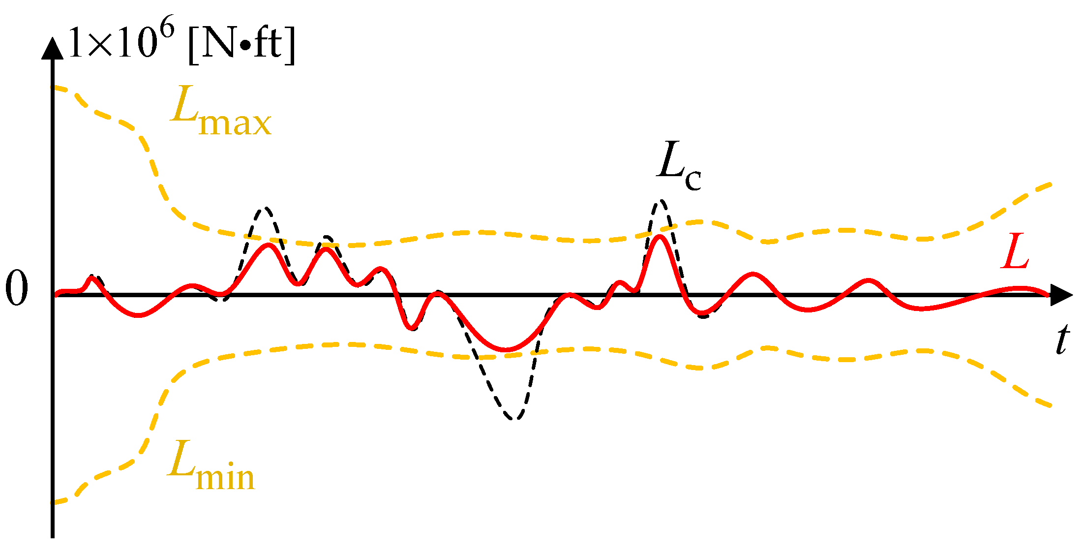
Figure 2 introduces the relationship between the AMB of $L$ and $L_{\mathrm{c}}$. It should be noted that the AMB in Figure 2 is calculated in an open loop by Algorithm 1, meaning it changes in real-time with the $\alpha , \beta , alt, \rho , \upsilon , {\upsilon }_{\mathrm{sound}}, p, q, r$ but does not feed back to the controller to participate in the PCR. Because $L_{\mathrm{c}}$ is unrestricted in this situation, $L_{\mathrm{c}}$ may cross over the AMB envelope. At the same time, $L$ often cannot perfectly match $L_{\mathrm{c}}$, which is caused by control allocation errors. Additionally, without a compensation loop, there is a gap between the peaks of $L$ and AMB. This means that the aerodynamic performance of the drone cannot be fully utilized.

Algorithm 1. AMB algorithm

function $\left[u_{\max }, u_{\min }\right]=\mathrm{AMB}\left(\alpha , \beta , alt, \rho , \upsilon , {\upsilon }_{\mathrm{sound}}, p, q, r, x_{\mathrm{ac}}, x_{\mathrm{cg}}\right)$

$\mathrm{Set}: {\alpha }_i^{\max }, {\alpha }_i^{\min }, {\beta }_i^{\max }, {\beta }_i^{\min }, al{t}_i^{\max }, al{t}_i^{\min }, V_i^{\max }, V_i^{\min }, {\delta }_{\max }, {\delta }_{\min }$

$\mathrm{Initialize}: b, \overline{c}, m, I_{xx}, I_{yy}, I_{zz}, I_{xz}, S_{\mathrm{ref}}, l_{\mathrm{tv}}$

$\mathrm{for} n=L, M, N, Y, Z$

$f_{\mathrm{Cn}}\left(\delta \right)=0$

$\mathrm{for} i=19$

$\alpha =\mathrm{sat}\left({\alpha }_i^{\max }, {\alpha }_i^{\min }\right), \beta =\mathrm{sat}\left({\beta }_i^{\max }, {\beta }_i^{\min }\right)$

$alt=\mathrm{sat}\left(al{t}_i^{\max }, al{t}_i^{\min }\right), V=\mathrm{sat}\left({\upsilon }_i^{\max }, {\upsilon }_i^{\min }\right)$

$p_0=p/\upsilon , q_0=q/\upsilon , r_0=r/\upsilon$

$\overline{q}=\rho {\upsilon }^2/2, Ma=\upsilon /{\upsilon }_{\mathrm{sound}}$

$f_{\mathrm{Cn}, i}\left(\delta \right)=\mathrm{Linear} \mathrm{interpolation}\left(\alpha , \beta , alt, \mathrm{{\rm M}}, p_0, q_0, r_0, \overline{q}\right)$

$\mathrm{or}$

$f_{\mathrm{Cn}, i}\left(\delta \right)=\mathrm{Cubic-spline} \mathrm{interpolation}\left(\alpha , \beta , alt, \mathrm{{\rm M}}, p_0, q_0, r_0, \overline{q}\right)$

$f_{\mathrm{Cn}}\left(\delta \right)=f_{\mathrm{Cn}}\left(\delta \right)+f_{\mathrm{Cn}, i}\left(\delta \right)$

$\mathrm{end} \mathrm{for}$

${\mathrm{C}}_{\mathrm{n-max}/\min }\left({\delta }_n\right)=\mathrm{fmincon}\left(f_{\mathrm{Cn}}\left(\delta \right), {\delta }_{\max }, {\delta }_{\min }, {\delta }_0\right)$

$\mathrm{end} \mathrm{for}$

$L_{\max /\min }=\overline{q}{b}_{\mathrm{ref}}{S}_{\mathrm{ref}}{\mathrm{C}}_{L\max /\min }$

$M_{\max /\min }=\overline{q} \overline{c}{S}_{\mathrm{ref}}{\mathrm{C}}_{M\max /\min }+\overline{q}\left(x_{\mathrm{ac}}-x_{\mathrm{cg}}\right)S_{\mathrm{ref}}{\mathrm{C}}_{Z\max /\min }$

$N_{\max /\min }=\overline{q}{b}_{\mathrm{ref}}{S}_{\mathrm{ref}}{\mathrm{C}}_{N\max /\min }-\overline{q}\left(x_{\mathrm{ac}}-x_{\mathrm{cg}}\right)S_{\mathrm{ref}}{\mathrm{C}}_{Y\max /\min }$

$\mathrm{return}: u_{\max }=\left[L_{\max }, M_{\max }, N_{\max }\right], u_{\min }=\left[L_{\min }, M_{\min }, N_{\min }\right]$

$\mathrm{end} \mathrm{function}$

3.2. Flight Performance Assurance System Design with AMB

The first design target of the FPA system in this article is to enable the flight controller to generate aerodynamic moment tracking signals according to its capabilities. In other words, the control effect of FPA is attitude-angle constraint control when mapping to the attitude loop, while AMB corresponds to the flight envelope. This flight envelope protection system is able to prevent loss-of-control-related accidents and improve flight safety [14]. To sum up, it is meaningful to enable the flight controller to perform aerodynamic moment commands according to its capabilities.

The output of the AMB algorithm can be defined as follows:

$$U\left(\alpha , \beta , alt, \rho , \mathrm{{\rm M}}, p, q, r\right)=\left[\begin{array}{ccc}{L}_{\max }& M_{\max }& N_{\max }\\ L_{\min }& M_{\min }& N_{\min }\end{array}\right]$$

(17)

The common anti-saturation processing strategies follow two core ideas. Firstly, the anti-saturation strategy does not work when the controlled quantity is within the AMB envelope. The second is to take the boundary value corresponding to the current flight state when the controlled quantity crosses the AMB envelope. This anti-saturation strategy is expressed by the following equation:

$$u_{\mathrm{ref}}=\left[\begin{array}{l}{L}_{\mathrm{ref}}\\ M_{\mathrm{ref}}\\ N_{\mathrm{ref}}\end{array}\right]=\left[\begin{array}{l}\max \left(L_{\min }, \min \left(L_{\mathrm{c}}, L_{\max }\right)\right)\\ \max \left(M_{\min }, \min \left(M_{\mathrm{c}}, M_{\max }\right)\right)\\ \max \left(N_{\min }, \min \left(N_{\mathrm{c}}, N_{\max }\right)\right)\end{array}\right]$$

(18)

Instead of $u_{\mathrm{ref}}$, a new anti-saturation strategy is adopted as follows:

$$u_{\mathrm{fpa}}=\left[\begin{array}{c}{L}_{\mathrm{fpa}}\\ M_{\mathrm{fpa}}\\ N_{\mathrm{fpa}}\end{array}\right]=\left[\begin{array}{c}{L}_c-d_L\epsilon (d_L)\mathrm{sech}\left(\cot \frac{\left(d_L+d_1\right)\pi }{2d_1}\right)\\ M_c-d_M\epsilon (d_M)\mathrm{sech}\left(\cot \frac{\left(d_M+d_2\right)\pi }{2d_2}\right)\\ N_c-d_N\epsilon (d_N)\mathrm{sech}\left(\cot \frac{\left(d_N+d_3\right)\pi }{2d_3}\right)\end{array}\right]$$

(19)

where $d_L,d_M,d_N$ describe how dangerous the current state is, $\mathrm{sech}\left(\cot \left(*\right)\right)$ describes how effective the protection will be by adjusting $d_1,d_2,d_3$. Take $L_{\mathrm{fpa}}$ as an example, where

$$d_L=\min \left(\left|L_{\max }-L\right|, \left|L_{\min }-L\right|\right)$$

(20)

$$\epsilon (d_L)=\left\{\begin{array}{cc}1\hfill & ,d_L<d_0\\ 0& ,d_L\ge d_0\end{array}\right.$$

(21)

Compared with Equation (18), the advantages of the FPA are as follows: (1) the aggressiveness of FPA can be altered online by tuning the thresholds $d_0$ and $d_1,d_2,d_3$ without recalculating the whole AMS; (2) the modification to the command is predictive, which starts before reaching the envelope boundary; (3) the boundedness of the modification term is guaranteed, which completes the boundedness proof of AMS-NDI, as will be shown in Section 5. Moreover, the anti-saturation effect of FPA can be shown in Figure 3.

It is important to note that the control command, which exceed AMB, will result in tracking errors between actual aerodynamic torque and control commands. This also means that the maneuverability of TUAVs cannot be achieved. If this tracking error is handled in an open loop, it will also lead to impaired maneuverability or even loss of control. Therefore, it is necessary to design an error compensation system as follows:

$$\varsigma =\left[{\xi }_1\tanh {\epsilon }_1; {\xi }_2\tanh {\epsilon }_2;{\xi }_3\tanh {\epsilon }_3\right]$$

(22)

where $\varsigma$ is the error compensation term, ${\xi }_i>0, i=1, 2, 3$ is the parameter to be designed, and ${\epsilon }_i$ is the state variable of the following error compensation system:

$$\left\{\begin{array}{l}{\dot{\epsilon }}_1=\left[-{\kappa }_1\tanh {\epsilon }_1+\Delta L\right]{\xi }_1^{-1}{\cosh }^2{\epsilon }_1\\ {\dot{\epsilon }}_2=\left[-{\kappa }_2\tanh {\epsilon }_2+\Delta M\right]{\xi }_2^{-1}{\cosh }^2{\epsilon }_2\\ {\dot{\epsilon }}_3=\left[-{\kappa }_3\tanh {\epsilon }_3+\Delta N\right]{\xi }_3^{-1}{\cosh }^2{\epsilon }_3\end{array}\right.$$

(23)

where ${\kappa }_i>0$ is the parameter to be designed, $\Delta L=L_{\mathrm{fpa}}-L_{\mathrm{c}}$, $\Delta M=M_{\mathrm{fpa}}-M_{\mathrm{c}}$, $\Delta N=N_{\mathrm{fpa}}-N_{\mathrm{c}}$.

4. FPA-NDI Controller Design

The structure of the FPA-NDI control system is shown in Figure 4.

From Figure 4, we can find that the essence of AMB plays the role of an observer, which feeds back the observation results to the NDI controller through FPA and influences the control command. It should be noted that, since the control allocation algorithm is not the focus of this paper, this section does not introduce the control algorithm in detail. The control allocation algorithm referenced by the control system originates from an incremental nonlinear control allocation proposed by the author’s team [13].

4.1. Attitude Control

The goal of the flight control system is to design a pseudo command $u_{\mathrm{c}}$ so that the following three-channel second-order systems can stably track the command signal,

$$\left\{\begin{array}{l}{\dot{\tilde{x}}}_1={\dot{x}}_1-{\dot{x}}_{1,\mathrm{d}}=f_1+G_1{x}_{2,\mathrm{c}}-{\dot{x}}_{1,\mathrm{d}}\\ {\dot{\tilde{x}}}_2={\dot{x}}_2-{\dot{x}}_{2,\mathrm{d}}=f_2+G_{2}u-{\dot{x}}_{2,\mathrm{d}}\end{array}\right.$$

(24)

where ${\tilde{x}}_1$ and ${\tilde{x}}_2$ are the tracking errors for the slow period and the fast period, respectively. To track the command signal $x_{1,\mathrm{d}}={\left[{\mu }_{\mathrm{d}}, {\alpha }_{\mathrm{d}}, {\beta }_{\mathrm{d}}\right]}^{\mathrm{T}}$, the virtual control law designed for the slow-period model $x_1$ is

$$x_{2,\mathrm{c}}=G_1^{-1}\left(v_1-f_1+{\dot{x}}_{1,\mathrm{d}}\right)$$

(25)

where $v_1$ is the linear control law to be designed. The pseudo-linear system is obtained by substituting the virtual control law $x_{2,\mathrm{c}}$ into Equation (10):

$${\dot{x}}_1=v_1+{\dot{x}}_{1,\mathrm{d}}$$

(26)

Then, the linear control law $v_1$ is designed by the LQR method,

$$\left\{\begin{array}{l}{v}_1=-R_1^{-1}{R}_2^T{P}_{1}x+R_1^{-1}{R}_2^T\overline{g}\\ \overline{g}={\left[P_1{R}_2{R}_1^{-1}{R}_2^T-R_3^T\right]}^{-1}{R}_4^T{Q}_1{x}_{1,\mathrm{d}}\end{array}\right.$$

(27)

where, $R_1$, $P_1$, $Q_1$ are symmetric positive constant matrices, and $P_1$ satisfies the Riccati equation:

$$P_1{R}_3+R_3^T{P}_1-P_1{R}_2{R}_1^{-1}{R}_2{P}_1+R_4^T{Q}_1{R}_4=0$$

(28)

where $R_2=R_4=E$, $R_3=0$, so the linear control law $v_1$ can be obtained:

$$v_1=P_1^{-1}{Q}_1\left(x_{1,\mathrm{d}}-x_1\right)$$

(29)

Filter the virtual control signal $x_{2,\mathrm{c}}$ to obtain the command signal $x_{2,\mathrm{d}}$ and its first derivative ${\dot{x}}_{2,\mathrm{d}}$. To track the command signal $x_{2,\mathrm{d}}$, based on the backstepping method, the NDI pseudo command $u_{\mathrm{c}}$ designed for the fast-period model $x_2$ is:

$$u_{\mathrm{c}}=G_2^{-1}\left(v_2-f_2+{\dot{x}}_{2,\mathrm{d}}-G_1{\tilde{x}}_1\right)$$

(30)

where $v_2$ is the linear control law to be designed.

Substituting the control instruction $u_{\mathrm{c}}$ into Equation (10), the pseudo-linear system is obtained:

$${\dot{x}}_2=v_2+{\dot{x}}_{2,\mathrm{d}}$$

(31)

Then, the linear control law $v_2$ is designed by the LQR method:

$$\left\{\begin{array}{l}{v}_2=-R_5^{-1}{R}_2^T{P}_{2}x+R_5^{-1}{R}_2^T\overline{g}\\ \overline{g}={\left[P_2{R}_2{R}_5^{-1}{R}_2^T-R_3^T\right]}^{-1}{R}_4^T{Q}_2{x}_{2,\mathrm{d}}\end{array}\right.$$

(32)

where $R_5$, $P_2$, $Q_2$ are symmetric positive constant matrices, $P_2$ satisfies the Riccati equation:

$$P_2{R}_3+R_3^T{P}_2-P_2{R}_2{R}_5^{-1}{R}_2{P}_2+R_4^T{Q}_2{R}_4=0$$

(33)

where $R_2=R_4=E$, $R_3=0$, so the linear control law $v_2$ can be obtained:

$$v_2=P_2^{-1}{Q}_2\left(x_{2,\mathrm{d}}-x_2-\varsigma \right)$$

(34)

where $\varsigma$ is the error compensation term. It is important to emphasize that, unlike traditional NDI controllers, the FPA forms a closed loop with the NDI controller by the $\varsigma$ in Equation (34). This not only prevents PCR through AMB, but also allows the design goals of the FPA system to be realized. This will provide a pathway for improving the performance of the NDI controller.

4.2. Stability Analysis

Theorem 1.

When the model of TUAVs (15) satisfies the above assumptions and is under the control of control commands (25) and (30), the closed-loop system has the following characteristics: 

(1) 

The state tracking error will gradually converge, which satisfies $\underset{t\to \infty }{\lim }\left(x_1-x_{1,\mathrm{d}}\right)=0$;

(2) 

The state variable ${\epsilon }_i$ in the compensation system (23) is bounded and the aerodynamic torque command constraint is not violated.

Proof of Theorem 1.

(1)

Firstly, the stability of the fast-period and slow-period models of the system under $u_{\mathrm{c}}$ is proved, and the radially unbounded positive definite Lyapunov function is designed as follows:

$$W_1=\frac{1}{2}\left({\tilde{x}}_1^{\mathrm{T}}{\tilde{x}}_1+{\tilde{x}}_2^{\mathrm{T}}{\tilde{x}}_2\right)$$

(35)

where $W_1$ is positive definite. The first order derivative of time $t$ along Equation (27) for $W_1$ is obtained:

$$\begin{array}{c}{\dot{W}}_1={\tilde{x}}_1^{\mathrm{T}}\left[f_1+G_1{x}_{2,\mathrm{c}}-{\dot{x}}_{1,\mathrm{d}}\right]+{\tilde{x}}_2^{\mathrm{T}}\left[f_2+G_2{u}_{\mathrm{c}}-{\dot{x}}_{2,\mathrm{d}}\right]\\ \hspace{1em}\hspace{1em}\hspace{1em}\hspace{1em}\hspace{1em}\hspace{1em}\hspace{1em}\hspace{1em}\hspace{1em}\hspace{1em}\hspace{1em}\hspace{1em} ={\tilde{x}}_1^{\mathrm{T}}\left[f_1+G_1{x}_{2,\mathrm{c}}+G_1\left({\rho }_1+{\tilde{x}}_2\right)-{\dot{x}}_{1,\mathrm{d}}\right]+{\tilde{x}}_2^{\mathrm{T}}\left[f_2+G_2{u}_{\mathrm{c}}+G_2\left({\rho }_2+\tilde{u}\right)-{\dot{x}}_{2,\mathrm{d}}\right]\hfill \end{array}$$

(36)

where ${\rho }_1$ and ${\rho }_2$ are the filtering errors generated by the command filter, and $\tilde{u}=u-u_{\mathrm{c}}=M-M_{\mathrm{c}}$ is the control allocation error. Substituting Equations (24) and (30) into the above equation yields:

$$\begin{array}{c}{\dot{W}}_1={\tilde{x}}_1^{\mathrm{T}}\left[f_1+v_1-f_1+{\dot{x}}_{1,\mathrm{d}}+G_1\left({\rho }_1+{\tilde{x}}_2\right)-{\dot{x}}_{1,\mathrm{d}}\right]+\\ \hspace{1em}\hspace{1em}\hspace{1em}\hspace{1em}\hspace{1em}\hspace{1em}\hspace{1em}\hspace{1em}\hspace{1em}\hspace{1em}{\tilde{x}}_2^{\mathrm{T}}\left[f_2+v_2-f_2+{\dot{x}}_{2,\mathrm{d}}+G_2\left({\rho }_2+\tilde{u}\right)-{\dot{x}}_{2,\mathrm{d}}-G_1{\tilde{x}}_1\right]\hfill \\ \hspace{1em}\hspace{1em}\hspace{1em}\hspace{1em}\hspace{1em}\hspace{1em}\hspace{1em}\hspace{1em}\hspace{1em}={\tilde{x}}_1^{\mathrm{T}}\left[-P_1^{-1}{Q}_1{\tilde{x}}_1+G_1{\rho }_1\right]+{\tilde{x}}_2^{\mathrm{T}}\left[-P_2^{-1}{Q}_2\left({\tilde{x}}_2+e_{\mathrm{cmp}}\right)+G_2\left({\rho }_2+\tilde{u}\right)\right]\hfill \\ \hspace{1em}\hspace{1em}\hspace{1em}\hspace{1em}\hspace{1em}\hspace{1em}\hspace{1em}\le -{\lambda }_1{‖{\tilde{x}}_1‖}^2-{\lambda }_2{‖{\tilde{x}}_2‖}^2-{\lambda }_2\xi ‖{\tilde{x}}_2‖+‖{\tilde{x}}_1‖G_1{\rho }_1+‖{\tilde{x}}_2‖G_2\left({\rho }_2+\tilde{u}\right)\end{array}$$

(37)

where ${\lambda }_1$ and ${\lambda }_2$ are the minimum eigenvalues of matrices $P_1^{-1}{Q}_1$ and $P_2^{-1}{Q}_2$, respectively. Therefore, it is possible to use a reasonable design of control parameters to achieve global asymptotic boundedness for Equation (9) when the filtering errors at each level and the control allocation error are bounded. The state tracking error of the slow-period model $x_1$ and the tracking command converge when ${\dot{W}}_1\le 0$ is proved. Therefore, the first part of Theorem 1 is proved.

(2)

Assuming that there is a constant vector $\overline{\omega }={\left[{\overline{\omega }}_1, {\overline{\omega }}_2, {\overline{\omega }}_3\right]}^T\ge 0$, which satisfies $\left|u_{\mathrm{fpa}}-u_c\right|\le \overline{\omega }$, $u_{\mathrm{fpa}}={\left[L_{\mathrm{fpa}}, M_{\mathrm{fpa}}, N_{\mathrm{fpa}}\right]}^{\mathrm{T}}$, the compensation system parameter $\kappa >\overline{\omega }$ is set. For the compensation system (22), the Lyapunov function is designed as follows:

$$W_2=\frac{{\xi }_1{\epsilon }_1^2}{2}$$

(38)

The first derivative of time $t$ along Equation (23) for $W_2$ can be obtained:

$$\begin{array}{c}{\dot{W}}_2=\left[-{\kappa }_1{\epsilon }_1\tanh {\epsilon }_1+{\epsilon }_1\left(M_{x-\mathrm{fpa}}-M_{xc}\right)\right]{\cosh }^2{\epsilon }_1\\ \hspace{1em}\hspace{1em}\hspace{1em}\le \left({\kappa }_1\left|{\epsilon }_1\right|-{\kappa }_1{\epsilon }_1\tanh {\epsilon }_1-{\kappa }_1\left|{\epsilon }_1\right|+{\overline{\omega }}_1\left|{\epsilon }_1\right|\right){\cosh }^2{\epsilon }_1\hfill \\ \hspace{1em}\hspace{1em}\hspace{1em}\le \left[0.2785{\kappa }_1-\left({\kappa }_1-{\overline{\omega }}_1\right)\left|{\epsilon }_1\right|\right]{\cosh }^2{\epsilon }_1\hfill \end{array}$$

(39)

Therefore, if $\left|{\epsilon }_1\right|>0.2785{\kappa }_1{\left({\kappa }_1-{\overline{\omega }}_1\right)}^{-1}$, then ${\dot{W}}_2<0$ contradicts the above discussion. Therefore, $\forall t\ge 0$, ${\epsilon }_1$ is contained in the compact set $\left\{{\epsilon }_1\left|\left|{\epsilon }_1\right|\le 0.2785{\kappa }_1{\left({\kappa }_1-{\overline{\omega }}_1\right)}^{-1}\right.\right\}$ and ${\epsilon }_1$ is bounded. Similarly, for $\forall t\ge 0$, $\epsilon$ is contained in a compact set $\left\{\epsilon \left|\left|\epsilon \right|\le 0.2785\kappa {\left(\kappa -\overline{\omega }\right)}^{-1}\right.\right\}$, which is proved by the second part of Theorem 1. So far, the design of the FPA-NDI controller and its stability proof have been introduced. □

5. Experiment Evaluation and Comparison

5.1. Scenario 1: Simulation Verification for Algorithm AMB

To verify the feasibility and accuracy of Algorithm 1, consider obtaining the AMB through open-loop online calculation. It should be noted that the AMB is not used for the closed-loop feedback as Figure 4 shows. The structure of the simulation is shown in Figure 5.

In scenario 1, the flight mission for the TUAVs to complete is set as a specified snake-shaped maneuver within 65 s, where $x_{1,\mathrm{d}}$ can be obtained from processed snake-shape flight data and is used as the tracking signal for the simulations. In addition, the parameters of the ICE aircraft are set as shown in

Table 2. ICE aircraft simulation parameters.

ICE Parameters	Value	Unit	Effectors	Action Range (deg)
$b_{\mathrm{ref}}$	$37.50$	$\mathrm{ft}$	lilef	[0, 40]
$\overline{c}$	$28.75$	$\mathrm{ft}$	rilef	[0, 40]
$m$	$\mathrm{32,750}$	$\mathrm{LBF}$	lolef	[−40, 40]
$I_{xx}$	$\mathrm{35,479}$	$\mathrm{slug}\cdot {\mathrm{ft}}^2$	rolef	[−40, 40]
$I_{yy}$	$\mathrm{78,451}$	$\mathrm{slug}\cdot {\mathrm{ft}}^2$	lamt	[0, 60]
$I_{zz}$	$\mathrm{110,627}$	$\mathrm{slug}\cdot {\mathrm{ft}}^2$	ramt	[0, 60]
$I_{xz}$	$-525$	$\mathrm{slug}\cdot {\mathrm{ft}}^2$	lele	[−30, 30]
$S_{\mathrm{ref}}$	$808.60$	${\mathrm{ft}}^2$	rele	[−30, 30]
$l_{\mathrm{tv}}$	$18.75$	$\mathrm{ft}$	lssd	[0, 60]
$x_{\mathrm{ac}}$	$38.84\%\overline{c}$		rssd	[0, 60]
$x_{\mathrm{cg}}$	$37.90\overline{c}$		pf	[−30, 30]

.

Furthermore, the NDI controller of scenario 1 is designed as follows:

$$\left\{\begin{array}{l}{x}_{2,\mathrm{c}}=G_1^{-1}\left(P_1^{-1}{Q}_1\left(x_{1,\mathrm{d}}-x_1\right)-f_1+{\dot{x}}_{1,\mathrm{d}}\right)\\ u_{\mathrm{c}}=G_2^{-1}\left(P_2^{-1}{Q}_2\left(x_{2,\mathrm{d}}-x_2\right)-f_2+{\dot{x}}_{2,\mathrm{d}}-G_1{\tilde{x}}_1\right)\end{array}\right.$$

(40)

where $P_1=\mathrm{diag}\left(3, 3, 3\right)$, $Q_1=\mathrm{diag}\left(9, 9, 9\right)$, $P_2=\mathrm{diag}\left(9, 9, 9\right)$, and $Q_2=\mathrm{diag}\left(81, 81, 81\right)$. The simulation results are shown in Figure 6, Figure 7, Figure 8 and Figure 9. Each of Figure 6, Figure 7 and Figure 8 contains both a global view and a local view.

First of all, $x_{1,\mathrm{d}}$ in Scenario 1 is restricted to obtain the mutation of ${\dot{x}}_{1,\mathrm{d}}$. Therefore, the maneuvering capability of ICE can be further challenged to more intuitively validate the effectiveness of AMB. It should be noted that the purpose of setting the tracking signal in this way is to generate multiple notable spikes for $L_{\mathrm{c}}, M_{\mathrm{c}}, N_{\mathrm{c}}$, which may exceed the envelope. This will help verify whether $L, M, N$ exceeds the AMB envelope at the same time.

Figure 6, Figure 7 and Figure 8 show that the curves of AMB can be successfully calculated online. Importantly, the envelope obtained from the online calculation successfully encapsulates the actual $L, M, N$, which are generated by the ICE model in the closed-loop control. It should be noted that the evolutions of $L, M, N$ closely follow the boundary of AMB, while part of the $L_{\mathrm{c}}, M_{\mathrm{c}}, N_{\mathrm{c}}$ exceeds the envelope. In addition, the AMB does not guide the control commands and $L_{\mathrm{c}}, M_{\mathrm{c}}, N_{\mathrm{c}}$ are not restricted. Therefore, Figure 6, Figure 7 and Figure 8 suggest that the AMB obtained from Algorithm 1 is reasonable.

Furthermore, combined with Figure 9, it can be concluded that every time $L, M, N$ approach AMB, it is accompanied by a rapid change in $\mu , \alpha , \beta$. It can also be inferred that $\alpha$ and $\beta$ play a crucial role in the calculation of AMB. The conclusion is that AMB follows the trend of $\alpha$, i.e., a smaller $\alpha$ leads to a wider envelope, further validating the algorithm’s rationality.

However, the simulation results in Figure 6, Figure 7, Figure 8 and Figure 9 are obtained under relatively relaxed conditions, which completes the snake-shaped maneuver in 65 s. So, it cannot be ignored that TUAVs may be more likely to lose control while increasing the maneuver intensity. Therefore, further simulation is required just as in Scenario 2.

5.2. Scenario 2: Comparison of NDI Controller Simulation

The purposes of Scenario 2 can be concluded as follows: (1) to further explore effective solutions for the control of TUAVs in rapid snake-shaped maneuver; (2) to validate the effectiveness of the FPA system and the advantages of the FPA-NDI controller; and (3) to further validate the effectiveness of AMB in more different situations. In addition, Scenario 2 keeps the parameters of the simulation the same as in Scenario 1, but sets the flight mission to complete the snake-shaped maneuver in 40 s. The FPA-NDI controller is designed as follows:

$$\left\{\begin{array}{l}{x}_{2,\mathrm{c}}=G_1^{-1}\left(P_1^{-1}{Q}_1\left(x_{1,\mathrm{d}}-x_1\right)-f_1+{\dot{x}}_{1,\mathrm{d}}\right)\\ u_{\mathrm{c}}=G_2^{-1}\left(P_2^{-1}{Q}_2\left(x_{2,\mathrm{d}}-x_2-\varsigma \right)-f_2+{\dot{x}}_{2,\mathrm{d}}-G_1{\tilde{x}}_1\right)\end{array}\right.$$

(41)

In addition, the parameters of the error compensation system $\varsigma$ are set as ${\kappa }_1={\kappa }_2={\kappa }_3=K_u$, ${\xi }_1={\xi }_2={\xi }_3=100K_u$, where $K_u=1\times {10}^6$ represents the order of magnitude of the aerodynamic moment $L, M, N$.

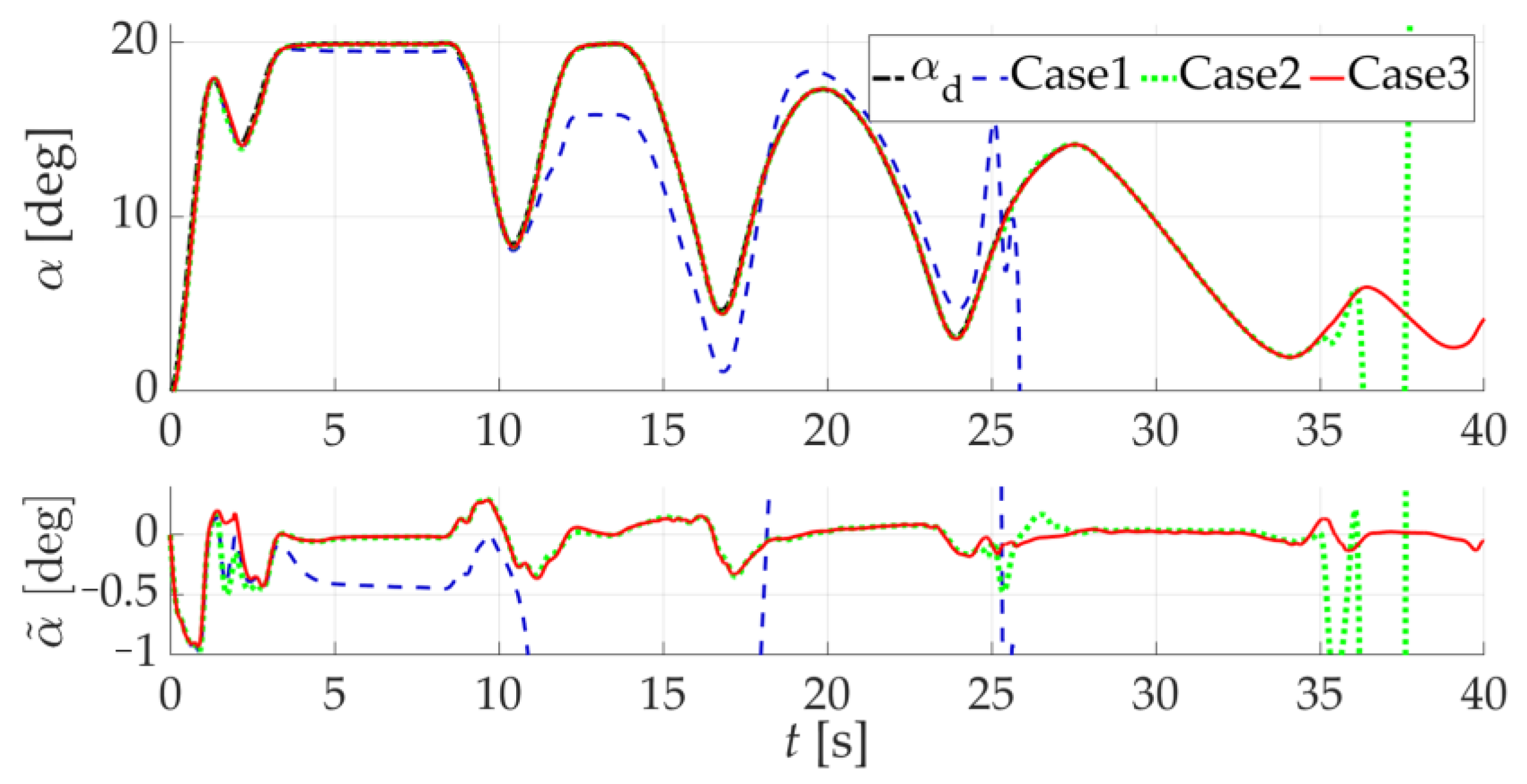
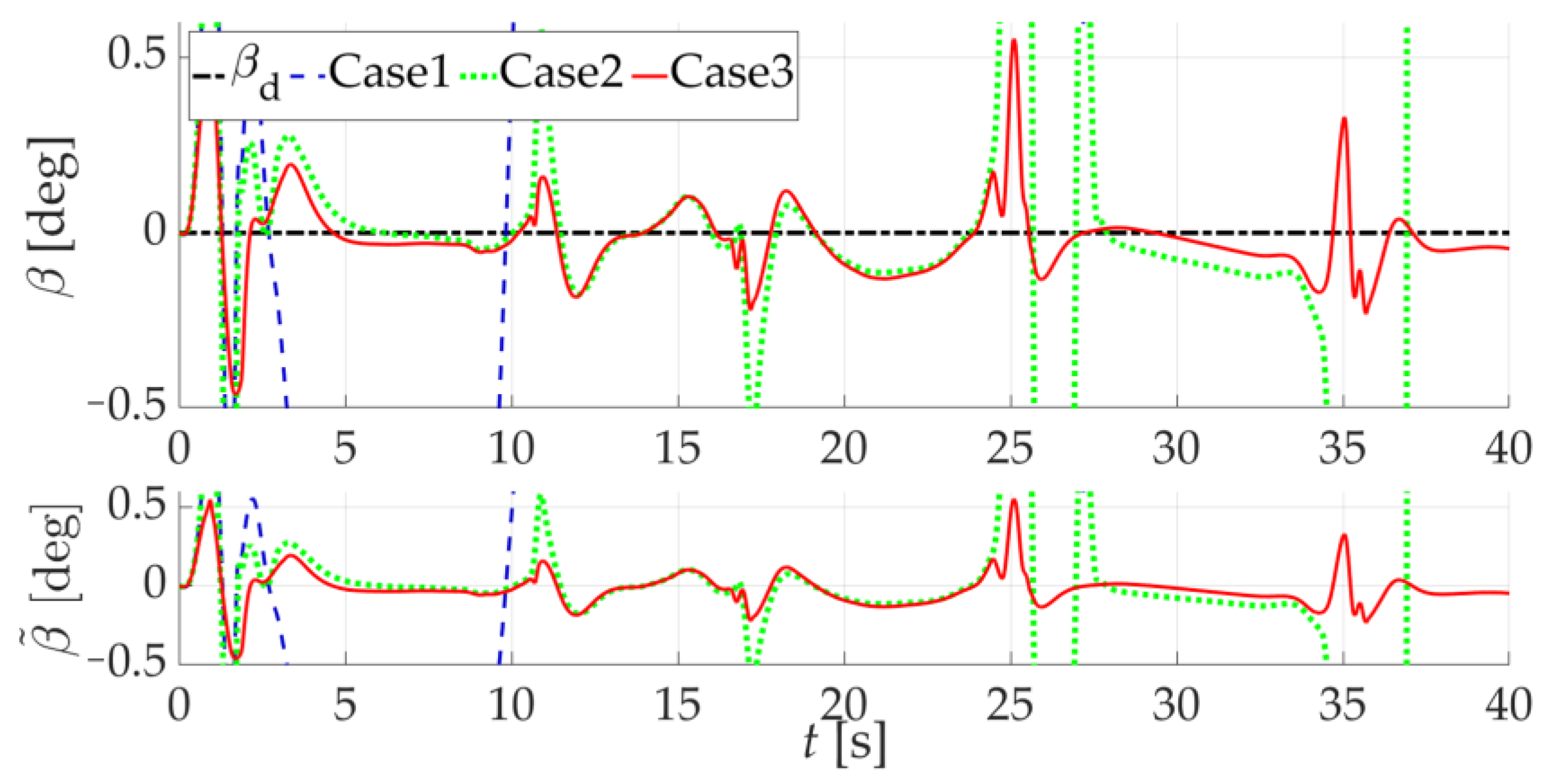
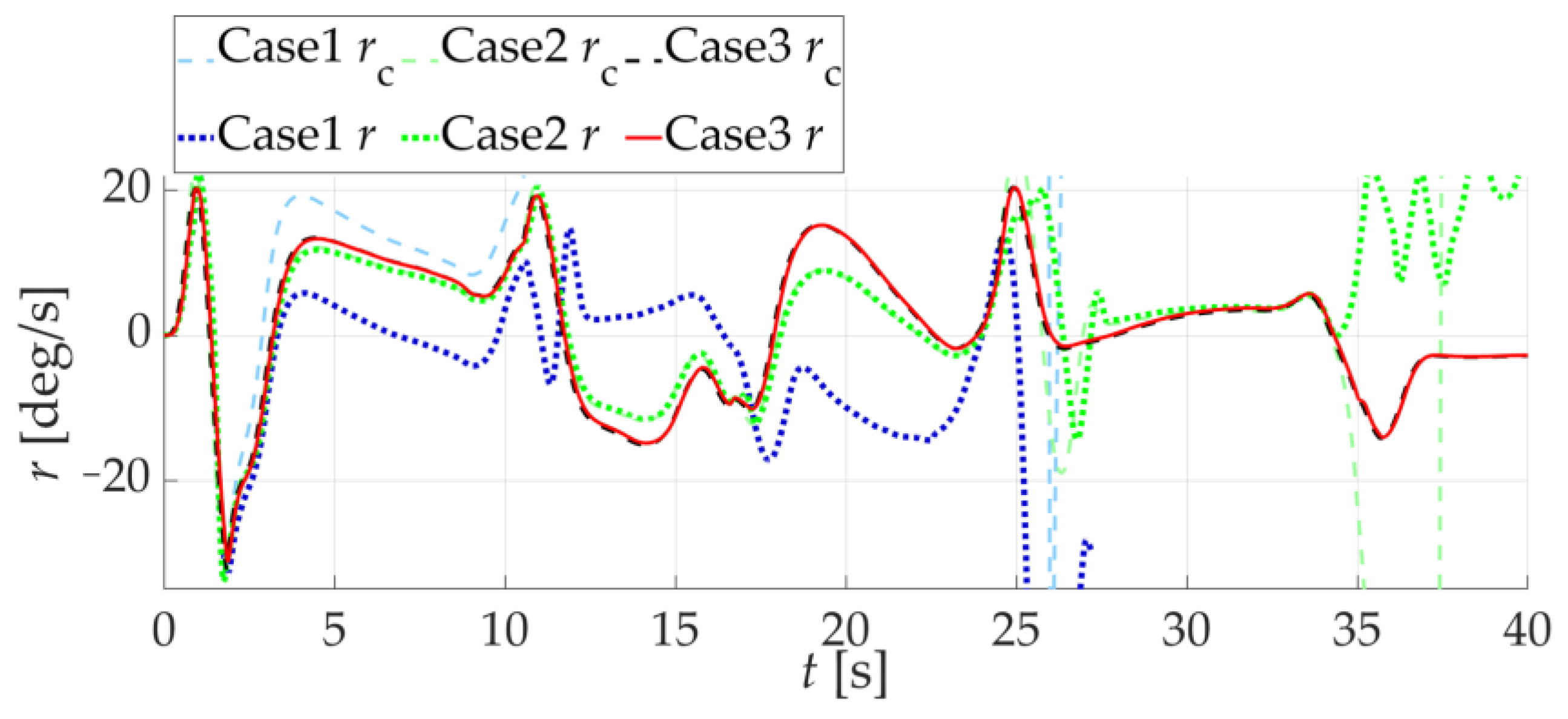
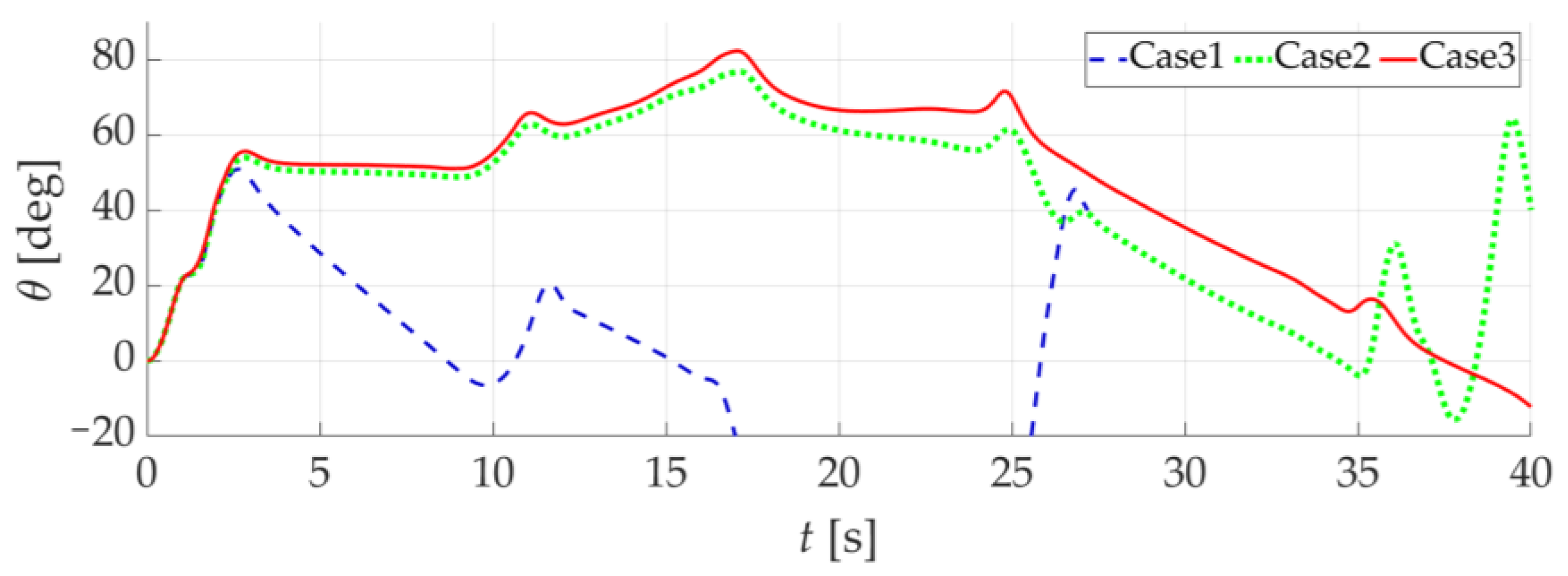
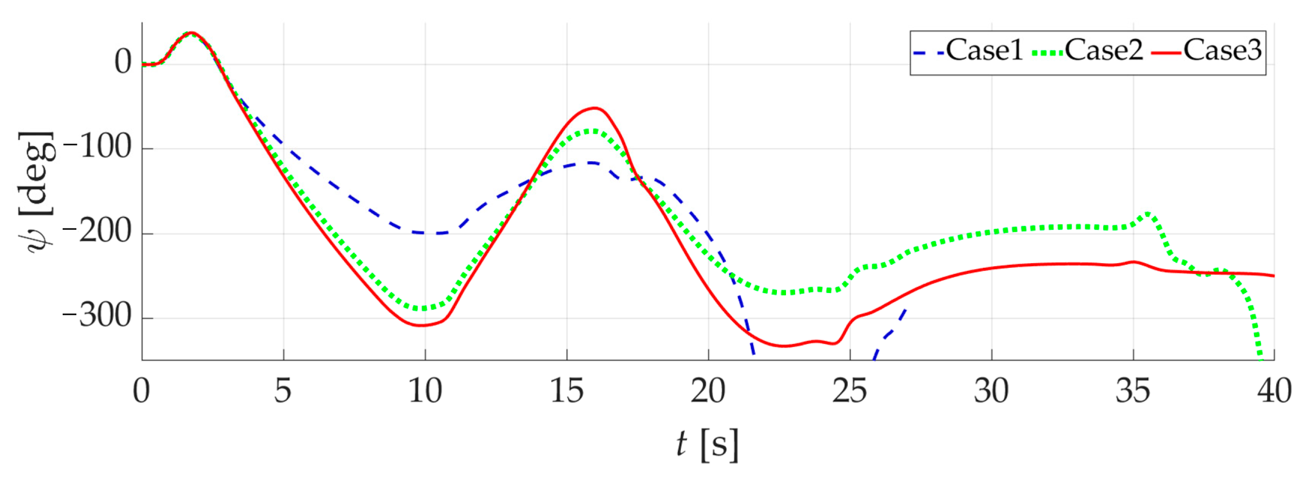
The simulation results are as shown in Figure 10, Figure 11, Figure 12, Figure 13, Figure 14, Figure 15, Figure 16, Figure 17, Figure 18, Figure 19, Figure 20, Figure 21, Figure 22, Figure 23, Figure 24, Figure 25, Figure 26, Figure 27 and Figure 28, in which Case 1 and Case 2 are control groups. The simulation results of Case 1 can be obtained by changing the flight mission to a 40-s snake-shaped maneuver while keeping the other parameters the same as in Scenario 1. Case 2 refers to the NDI-restricted control adopted from [14]. It should be noted that [14] restricts the extension of the constraint of $\mu , \alpha , \beta$ instead of $L, M, N$. So, it is necessary to extend the method of restricted control to $L, M, N$. Case 3 presents simulation results obtained under conditions identical to those of Case 1 and Case 2, with the only distinction being the controller design.

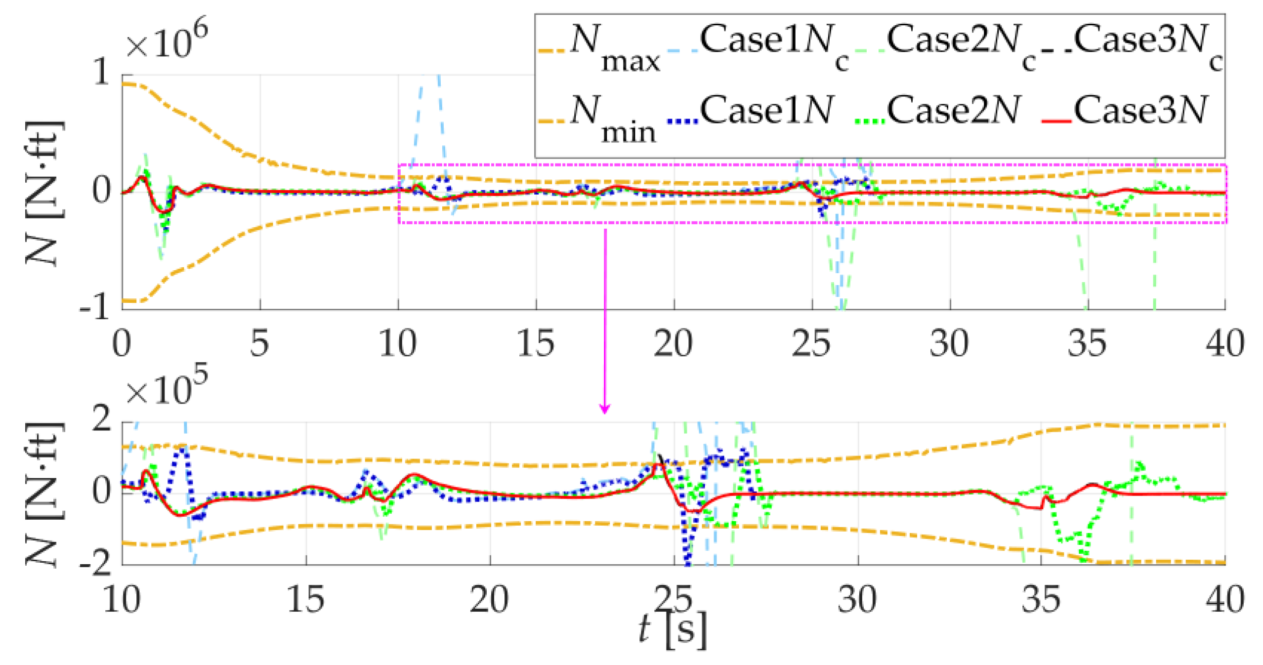
Figure 10, Figure 11 and Figure 12 and 22 show that Case 1 loses control at about 26 s, and Case 2 loses control at about 37 s. Meanwhile, Case 3 not only completes the snake-shaped maneuver, but also has a faster tracking speed and smaller tracking error. To expand on this, the $p, q, r$ in Case 1 has been unable to effectively track $p_{\mathrm{c}}, q_{\mathrm{c}}, r_{\mathrm{c}}$ at about 3 s, while Case 2 is at about 34 s. Together with Figure 17, Figure 18 and Figure 19, we can find that both the reasons for Case 1 and Case 2 are lacking enough $L, M, N$ compared with $L_{\mathrm{c}}, M_{\mathrm{c}}, N_{\mathrm{c}}$. It should be noted that the curves of the envelope in Figure 17, Figure 18 and Figure 19 represent AMB in Case 3. So, it is normal for $L, M, N$ of Case 1 and Case 2 to exceed the AMB. Because of the FPA system, FPA-NDI can not only generate a more seasonable tracking signal for $L, M, N$, but also generate enough ss through $\varsigma$. To sum up, the effectiveness of Case 3 has been validated. However, it seems that Case 2 can also complete the snake-shaped maneuvers from Figure 22. So, further analysis is necessary to further validate the superiority of Case 3.

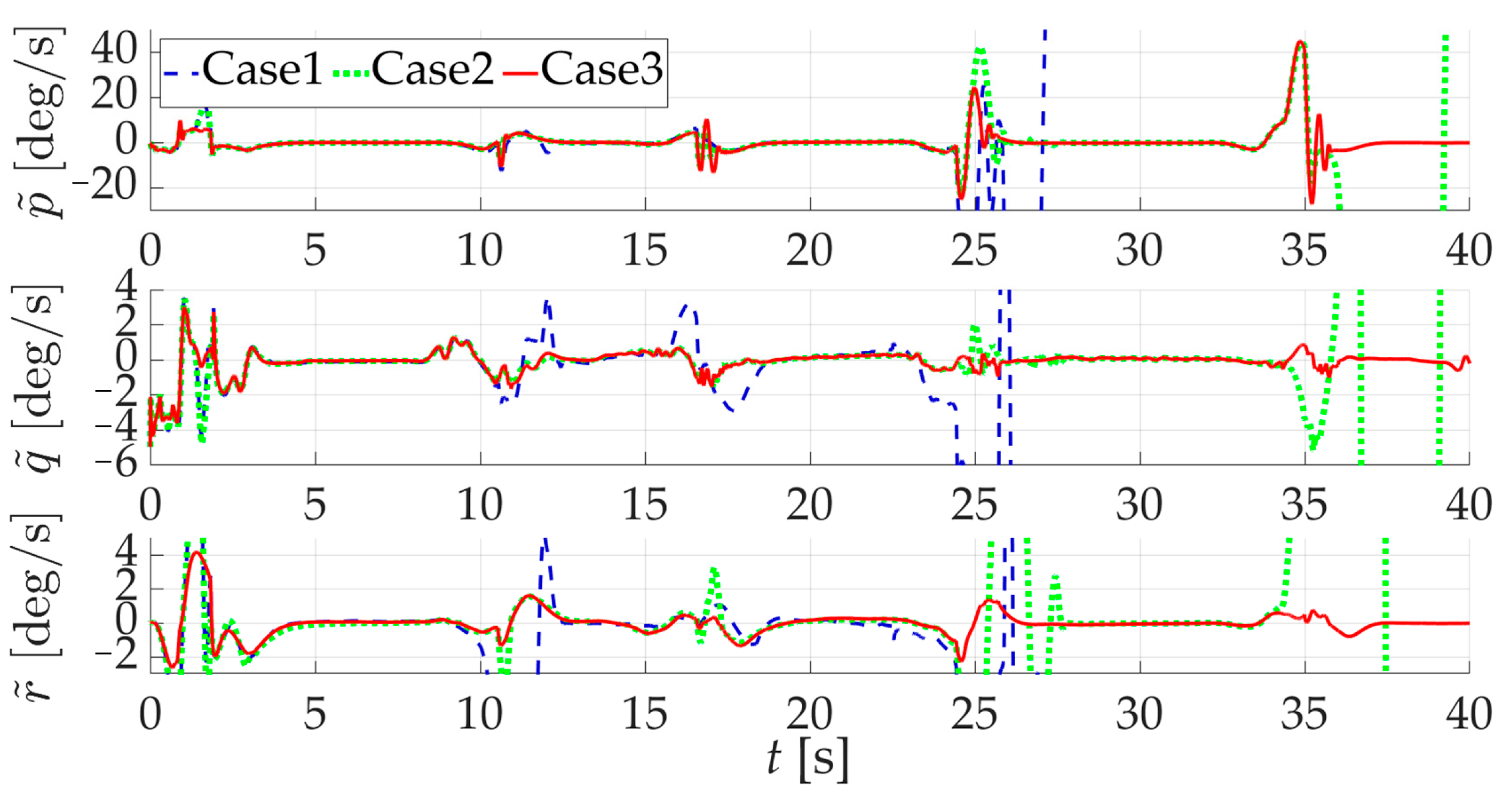
Due to the complexity of the snake-shaped trajectory in Case 3, Figure 22 contains four figures to display the flight trajectory more clearly. The first one is a three-dimensional trajectory map, and the remaining three are side views in three coordinate axis directions. We can find that, although Case 2 can also perform the maneuver, the complexity of its maneuvering trajectory is weaker than that of Case 3. Therefore, the flight security of ICE in Case 3 is better than in Case 2. In addition, we obtain the curves of $\varphi , \theta , \Psi$ to further describe the details of the ICE maneuver. Figure 23, Figure 24 and Figure 25 show that Case 2 rolls and yaws extremely fast after 35 s. Therefore, the snake-shaped maneuver of Case 2 loses control, in fact. The maneuver of Case 3 can be divided into three parts, where ICE turns around first and exits the dangerous airspace after completing the snake maneuver quickly.

Figure 13, Figure 14, Figure 15 and Figure 16 show that, during the snake-like maneuver, the ICE aircraft shakes violently at about 10 s, 17 s, 25 s, and 35 s. And the reasons for the loss of control in Case 1 and Case 2 are both due to the inability to regain stability after severe shaking. Moreover, Figure 13, Figure 14, Figure 15 and Figure 16 reveal that the growing $\tilde{p},\tilde{q},\tilde{r}$ will lead to the rapid saturation of $L,M,N$ in Figure 17, Figure 18 and Figure 19. This will make $u_{\mathrm{fpa}}-u_c$ increase rapidly so that the capability of the constrained compensator in Case 2 will be exceeded, which will result in the loss of control. In comparison, Figure 20 demonstrates that the designed FPA system can provide suitable $\varsigma$ for $\tilde{p},\tilde{q},\tilde{r}$. This will rapidly increase $L_{\mathrm{c}},M_{\mathrm{c}},N_{\mathrm{c}}$ while ensuring that $L,M,N$ remain within the AMB.

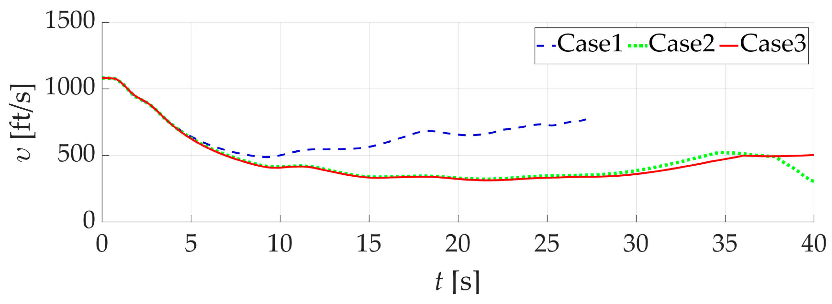
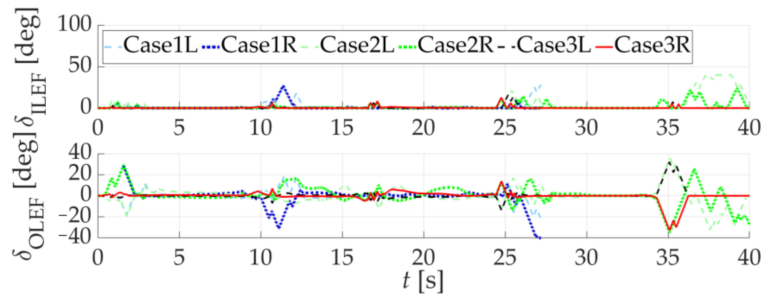
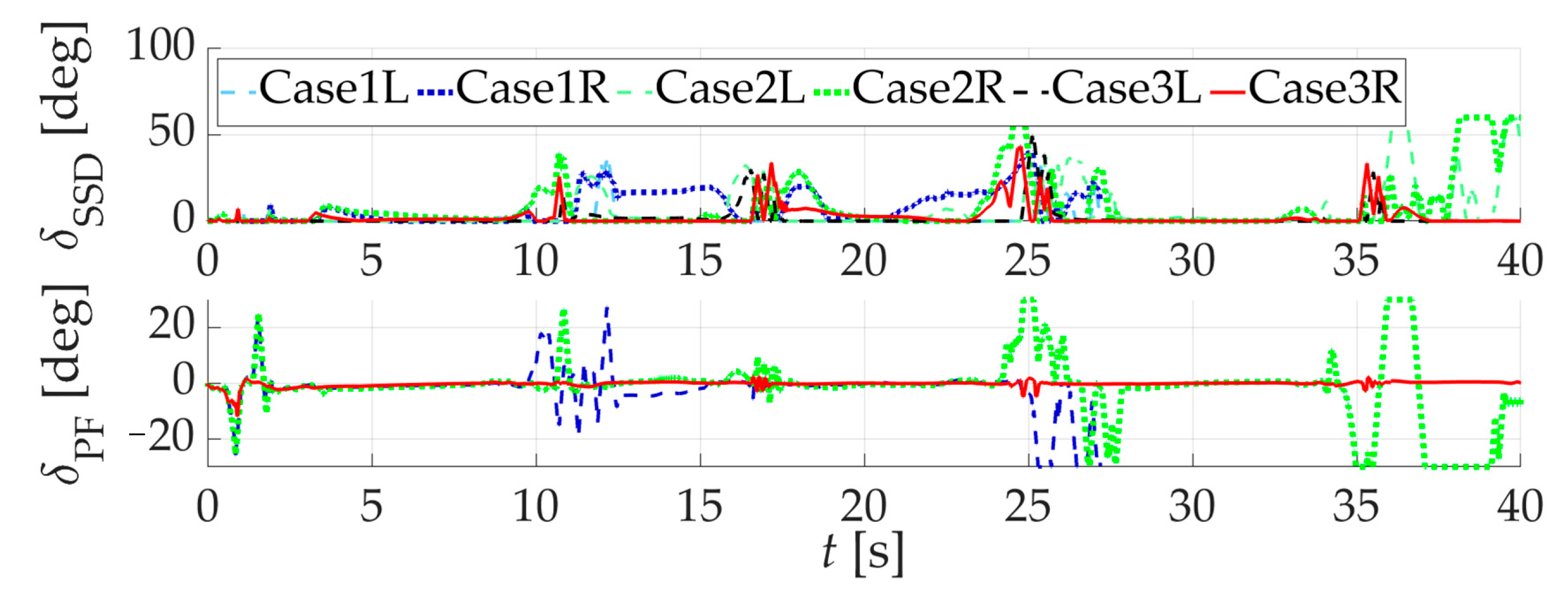
Additionally, Figure 21 describes the conversion of kinetic energy and potential energy throughout the entire maneuver process under limited thrust conditions. Figure 23, Figure 24 and Figure 25 present the actual control surface deflection of the ICE aircraft resulting from the aerodynamic moment commands of the PCR controller after being solved by the control allocation algorithm. But these are not the innovations in this paper, so we only briefly introduce them instead of providing further detailed analysis.

6. Conclusions

In this paper, a novel FPA-NDI controller was proposed and its performance in PCR control was demonstrated. To implement and test the controller, the model of ICE was introduced, which includes 11 effectors. In addition to the FPA-NDI controller, two other controllers were also tested on this ICE model, and the performance of all controllers was evaluated during the snake-shaped maneuver.

Firstly, in the aforementioned modeling scenario, a primary conclusion that the AMB algorithm was able to effectively calculate the envelope online can be drawn. Also, its feasibility and accuracy can be validated by comparing it with the curves of $L,M,N$, which were obtained in an open-loop simulation, and the ability of maneuver was apparently challenged. Additionally, the effectiveness and advantages of the FPA-NDI controller, which was built based on the AMB algorithm, were validated by comparative analysis. This means that the FPA system based on the AMB can achieve its design goals of a predictive boundary and compensating for deficiencies. Therefore, the design objectives outlined in the introduction were successfully achieved by the AMB algorithm and the FPA-NDI controller. In conclusion, the integration of the AMB algorithm with the PCR problem in flight control aids in exploring the maneuvering limits of TUAVs within specified constraints, thereby enhancing their maneuvering capabilities.

Before expounding on our future work, it should be noted that Algorithm 1 was conservative in determining AMS boundaries. In other words, the envelopes of the AMB may be larger than the capability boundary of the maneuver in reality. This is due to the inability of the algorithm to simultaneously obtain the envelopes of $L,M,N$ under the same set of effectors. Nonetheless, the AMB was enough to guide and solve the PCR problem. For future research, more precise flight control methods, such as the NDI/INDI controller, are planned, and it is apparent that the AMB is insufficient, so it requires further improvement and innovation.

References

- Shayan, K. Online Actor-Critic-Based Adaptive Control for a Tailless Aircraft with Innovative Control Effectors. In Proceedings of the AIAA Scitech 2021 Forum, Virtual, 11–21 January 2021. [Google Scholar]
- Harris, J.; Elliott, C.M.; Tallant, G. L1 Adaptive Nonlinear Dynamic Inversion Control for the Innovative Control Effectors Aircraft. In Proceedings of the AIAA SCITECH 2022 Forum, San Diego, CA, USA, 3–7 January 2022. [Google Scholar]
- Cong, J.; Hu, J.; Wang, Y.; He, Z.; Han, L.; Su, M. Fault-Tolerant Attitude Control Incorporating Reconfiguration Control Allocation for Supersonic Tailless Aircraft. Aerospace 2023, 10, 241. [Google Scholar] [CrossRef]
- Zhu, J.; He, R.; Tang, G.; Bao, W. Pendulum Maneuvering Strategy for Hypersonic Glide Vehicles. Aerosp. Sci. Technol. 2018, 78, 62–70. [Google Scholar] [CrossRef]
- Guo, Q.; Teng, L. Maneuvering Target Tracking with Multi-Model Based on the Adaptive Structure. IEEJ Trans. Electr. Electron. Eng. 2022, 17, 865–871. [Google Scholar] [CrossRef]
- Wan, J.; Ren, P.; Guo, Q. Application of Interactive Multiple Model Adaptive Five-Degree Cubature Kalman Algorithm Based on Fuzzy Logic in Target Tracking. Symmetry 2019, 11, 767. [Google Scholar] [CrossRef]
- Yu, X.; Luo, S.; Liu, H. Integrated Design of Multi-Constrained Snake Maneuver Surge Guidance Control for Hypersonic Vehicles in the Dive Segment. Aerospace 2023, 10, 765. [Google Scholar] [CrossRef]
- Maolin, W.; Shenghao, F.; Fei, L.; Renli, L.; Nan, Y. Research on Control Law Design of Fixed Wing Unmanned Aerial Vehicle in Aerobatic Maneuvers. In Proceedings of the 2022 34th Chinese Control and Decision Conference (CCDC), Hefei, China, 15–17 August 2022; pp. 4665–4670. [Google Scholar] [CrossRef]
- Lungu, M.; Flores, G.; Dinu, D.-A.; Ciuca, G.M. Autonomous Landing of Tailless, Blended Wing, and Variable Centre of Mass UAV Using Adaptive Control. In Proceedings of the 2022 8th International Conference on Control, Decision and Information Technologies (CoDIT), Istanbul, Turkey, 17–20 May 2022; pp. 112–117. [Google Scholar] [CrossRef]
- Yu, Z.; Li, Y.; Lv, M.; Pei, B.; Fu, A. Event-Triggered Adaptive Fuzzy Fault-Tolerant Attitude Control for Tailless Flying-Wing UAV with Fixed-Time Convergence. IEEE Trans. Veh. Technol. 2023, 1–12. [Google Scholar] [CrossRef]
- Nie, B.; Liu, Z.; Guo, T.; Fan, L.; Ma, H.; Sename, O. Design and Validation of Disturbance Rejection Dynamic Inverse Control for a Tailless Aircraft in Wind Tunnel. Appl. Sci. 2021, 11, 1407. [Google Scholar] [CrossRef]
- Stolk, A.R.J. Minimum Drag Control Allocation for the Innovative Control Effector Aircraft. Master’s Thesis, Delft University of Technology, Delft, The Netherlands, 2017. [Google Scholar]
- Su, M.; Hu, J.; Wang, Y.; He, Z.; Cong, J.; Han, L. A Multiobjective Incremental Control Allocation Strategy for Tailless Aircraft. Int. J. Aerosp. Eng. 2022, 2022, 6515234. [Google Scholar] [CrossRef]
- Yin, M.; Chu, Q.P.; Zhang, Y.; Niestroy, M.A.; De Visser, C.C. Probabilistic Flight Envelope Estimation with Application to Unstable Overactuated Aircraft. J. Guid. Control. Dyn. 2019, 42, 2650–2663. [Google Scholar] [CrossRef]
- He, Z.; Hu, J.; Wang, Y.; Cong, J.; Bian, Y.; Han, L. Attitude-Tracking Control for Over-Actuated Tailless UAVs at Cruise Using Adaptive Dynamic Programming. Drones 2023, 7, 294. [Google Scholar] [CrossRef]
- Durham, W.C. Attainable Moments for the Constrained Control Allocation Problem. J. Guid. Control. Dyn. 1994, 17, 1371–1373. [Google Scholar] [CrossRef]
- Kou, L.; He, S.; Li, Y.; Xiang, J. Constrained Control Allocation of a Quadrotor-Like Autonomous Underwater Vehicle. J. Guid. Control. Dyn. 2021, 44, 659–666. [Google Scholar] [CrossRef]
- Yu, Y.; Li, R.; Ji, W.; Lu, Z.; Tian, G. Refinements of the Dynamic Inversion Part of Hierarchical 4WIS/4WID Trajectory Tracking Controllers; SAE International: Detroit, MI, USA, 2023. [Google Scholar] [CrossRef]
- Ghobadi, M.; Shafaee, M.; Nadoushan, M.J. Reliability Approach to Optimal Thruster Configuration Design for Spacecraft Attitude Control Subsystem. J. Aerosp. Technol. Manag. 2020, 12, e2320. [Google Scholar] [CrossRef]
- Pfeifle, O.; Fichter, W. Incremental Control Allocation with Axis Prioritization on the Boundary of the Attainable Control Set. In Proceedings of the AIAA SciTech 2023 Forum, National Harbor, MD, USA, 23–27 January 2023; American Institute of Aeronautics and Astronautics: Reston, VA, USA, 2023. [Google Scholar] [CrossRef]
- Lu, Z.; Hong, H.; Diepolder, J.; Holzapfel, F. Maneuverability Set Estimation and Trajectory Feasibility Evaluation for eVTOL Aircraft. J. Guid. Control. Dyn. 2023, 46, 1184–1196. [Google Scholar] [CrossRef]
- Bolander, C.R.; Hunsaker, D.F.; Myszka, D.; Joo, J.J. Attainable Moment Set and Actuation Time of a Bio-Inspired Rotating Empennage. In Proceedings of the AIAA SCITECH 2022 Forum, San Diego, CA, USA, 3–7 January 2022. [Google Scholar]
- Zheng, F.; Liu, L.; Chen, Z.; Chen, Y.; Cheng, F. Hybrid Multi-Objective Control Allocation Strategy for Compound High-Speed Rotorcraft. ISA Trans. 2020, 98, 207–226. [Google Scholar] [CrossRef] [PubMed]
- Zhu, Z.; Guo, H.; Ma, J. Aerodynamic Layout Optimization Design of a Barrel-Launched UAV Wing Considering Control Capability of Multiple Control Surfaces. Aerosp. Sci. Technol. 2019, 93, 105297. [Google Scholar] [CrossRef]
- Lei, H.; Chen, B.; Liu, Y.; Lv, Y. Modified Kalman Particle Swarm Optimization: Application for Trim Problem of Very Flexible Aircraft. Eng. Appl. Artif. Intell. 2021, 100, 104176. [Google Scholar] [CrossRef]
- Zhang, N. Research on Command Allocation Method for Flying Wing Aircraft. IOP Conf. Ser. Mater. Sci. Eng. 2020, 887, 012020. [Google Scholar] [CrossRef]
- Qu, X.; Shi, J.; Zhou, H.; Zuo, L.; Lyu, Y. Reconfigurable Flight Control System Design for Blended Wing Body UAV Based on Control Allocation. In Proceedings of the 2018 18th International Conference on Control, Automation and Systems (ICCAS), PyeongChang, Republic of Korea, 17–20 October 2018. [Google Scholar]
- Matamoros, I.; De Visser, C.C. Incremental Nonlinear Control Allocation for a Tailless Aircraft with Innovative Control Effectors. In Proceedings of the 2018 AIAA Guidance, Navigation, and Control Conference, Kissimmee, FL, USA, 8–12 January 2018; American Institute of Aeronautics and Astronautics: Kissimmee, FL, USA, 2018. [Google Scholar] [CrossRef]
- Niestroy, M.A.; Dorsett, K.M.; Markstein, K. A Tailless Fighter Aircraft Model for Control-Related Research and Development. In Proceedings of the AIAA Modeling and Simulation Technologies Conference, Grapevine, TX, USA, 9–13 January 2017; American Institute of Aeronautics and Astronautics: Reston, VA, USA, 2017. [Google Scholar] [CrossRef]
- Wang, Z.; Zhang, J.; Yang, L.; Guo, X. Weighted Pseudo-Inverse Based Control Allocation of Heterogeneous Redundant Operating Mechanisms for DPC Aircraft. In Proceedings of the 2018 15th International Conference on Control, Automation, Robotics and Vision (ICARCV), Singapore, 18–21 November 2018; pp. 367–370. [Google Scholar] [CrossRef]
- Zhang, B.; Liu, D.; Liu, L.; Zhao, Y.; Sun, L.; Yao, Z. Path Prediction Method for Automotive Applications Based on Cubic Spline Interpolation. In Proceedings of the 2022 International Conference on Advanced Robotics and Mechatronics (ICARM), Guilin, China, 9–11 July 2022; pp. 1086–1091. [Google Scholar]
Figure 1.
Top view of ICE.
Figure 2.
AMB of that changes in real-time with flight states.
Figure 3.
Comparison of constraint effects between Equations (18) and (19).
Figure 4.
FPA-NDI control system.
Figure 5.
Simulation analysis of AMB.
Figure 6.
Calculation of and comparison with , .
Figure 7.
Figure 8.
Figure 9.
Curves of , , and .
Figure 10.
Comparative simulation results of and .
Figure 11.
Figure 12.
Figure 13.
Comparative simulation results of roll rate .
Figure 14.
Comparative simulation results of pitch rate .
Figure 15.
Comparative simulation results of yaw rate .
Figure 16.
Comparative simulation results of tracking errors , , .
Figure 17.
Comparative simulation results between and AMB.
Figure 18.
Figure 19.
Figure 20.
FPA system error compensation term .
Figure 21.
Comparative simulation results of .
Figure 22.
Snake-shaped maneuver flight trajectory with 4 perspectives.
Figure 23.
Figure 24.
Figure 25.
Figure 26.
Comparative simulation results of LEF rudder deviation.
Figure 27.
Comparative simulation results of SSD & PF rudders deviation.
Figure 28.
Comparative simulation results of AMT & ELE rudders deviation.