
UAV Photogrammetric Surveys for Tree Height Estimation

Department of Civil, Environmental Engineering and Architecture (DICAAR), 09123 Cagliari, Italy
*
Author to whom correspondence should be addressed.
Drones 2024, 8(3), 106; https://doi.org/10.3390/drones8030106
Submission received: 2 February 2024
/
Revised: 14 March 2024
/
Accepted: 18 March 2024
/
Published: 20 March 2024
(This article belongs to the Section Drones in Agriculture and Forestry)
Abstract
:In the context of precision agriculture (PA), geomatic surveys exploiting UAV (unmanned aerial vehicle) platforms allow the dimensional characterization of trees. This paper focuses on the use of low-cost UAV photogrammetry to estimate tree height, as part of a project for the phytoremediation of contaminated soils. Two study areas with different characteristics in terms of mean tree height (5 m; 0.7 m) are chosen to test the procedure even in a challenging context. Three campaigns are performed in an olive grove (Area 1) at different flying altitudes (30 m, 40 m, and 50 m), and one UAV flight is available for Area 2 (42 m of altitude), where three species are present: oleander, lentisk, and poplar. The workflow involves the elaboration of the UAV point clouds through the SfM (structure from motion) approach, digital surface models (DSMs), vegetation filtering, and a GIS-based analysis to obtain canopy height models (CHMs) for height extraction based on a local maxima approach. UAV-derived heights are compared with in-field measurements, and promising results are obtained for Area 1, confirming the applicability of the procedure for tree height extraction, while the application in Area 2 (shorter tree seedlings) is more problematic.
1. Introduction
Precision agriculture (PA) is defined as a particular agricultural management strategy based on the observations, measurements, and responses of a set of quantitative and qualitative variables affecting agricultural production [1]. The first step in the PA approach is the acquisition and collection of data from different sensors, such as optical multispectral and geophysical ones, to obtain a deep characterization of plants and monitor a crop [2]. Therefore, PA commonly includes a wide range of techniques and methodologies that need to be properly combined to develop increasingly sustainable agricultural management [3,4]. In this regard, the combination of data from different sources is bound to the proper management of the reference system, commonly handled through geographic information systems (GISs), which are highly suitable tools for multidisciplinary studies [5,6]. Among all, geophysics and geomatics techniques represent fundamental support tools for PA applications, giving essential information for cultivation protection and monitoring [7].
In particular, geophysical analyses involve the study of the chemical characteristics of plants and the shallow part of the subsoil, using ad hoc instruments, such as georadar systems [8,9]. On the other hand, geomatic techniques allow obtaining quantitative parameters describing the plants, in terms of height, crown extension, and volume. The use of global navigation satellite systems (GNSSs) in the agricultural field dates back to the 90s, with the development of farm machines equipped with GNSS receivers. However, the use of GNSS instruments to acquire field measurements cannot ensure high-density datasets without resulting in very time-consuming and expensive surveys [10]. Therefore, in this context, they are commonly employed as a support for other techniques. In the early 2000s, drones became the new major players in precision agriculture, being a very useful platform to transport different types of sensors (i.e., LiDAR, multi-spectral, and optical cameras). Indeed, the main advantages of using unmanned aerial vehicles (UAVs) are related to the fast performance and lower costs compared to other geomatic techniques [11,12].
Several studies addressed the use of UAV remotely sensed data for forestry or agricultural applications, mainly relying on LiDAR (light detection and ranging) datasets or multi-spectral imagery [9,13,14,15,16,17,18,19,20]. Moreover, most of the applications are framed in forest environments, where tall and dense trees are present, and the main focus is crown identification and classification [14,15,17,21,22,23,24]. On the other hand, recent studies have been conducted over areas with lower vegetation, using photogrammetric or LiDAR data sources [16,25,26,27,28,29,30]. In particular, tree height extraction exploiting UAV-acquired imagery has been addressed by several researchers, with different specific characteristics of the observed plants, providing promising results [14,21,23,31,32]. Compared with LiDAR point clouds, photogrammetric data are known to be generally noisier and less accurate since they do not provide information about the terrain surface but only the upper layer [14]. Conversely, information representing the ground level can be retrieved from LiDAR data by exploiting multi-return echoes penetrating the canopy [33,34]. This fact commonly ensures a better accuracy of the ground representation, which is crucial for a fair reconstruction of the 3D structure of vegetation [14]. Nevertheless, this benefit is obtained with more expensive instruments, requiring also more advanced carrying platforms.
Whatever the employed technique, analysis in the agricultural field generally relies on raster-based methods, through canopy height models (CHM), or others combining point clouds and raster data [35,36,37]. A CHM represents tree crowns and their heights from the ground; hence, it is commonly obtained as the difference between a digital surface model (DSM) and a related digital terrain model (DTM). The reference DTMs can be generated by exploiting automatic filters to identify the points representing the ground surface. Originally, the algorithms for vegetation filtering were designed for LiDAR datasets, although they can be employed also for photogrammetric applications [24]. Indeed, different software implements automatic filters for the vegetation that yet lead to better performances in forests rather than in areas with low trees [14,25,26,27]. However, fruit farmland or vineyards are characterized by the presence of sparse trees and relatively low heights, ranging approximately from 1 m to 4 m [38]. A similar situation concerns soils contaminated by pollutants or heavy metals undergoing phytoremediation or reclamation by planting trees or shrubs that can improve the chemical and physical characteristics of the soils and reduce the pollution level [39,40]. These latter contexts are commonly characterized by very low vegetation, in the order of half a metre, and height extraction applications in these contexts are poorly available in the literature, except for LiDAR. Some possible limitations of the SfM algorithm for the extraction of the height of low trees are addressed in the study by Matsuura et al. (2023) [41], developing a stereo-matching-based methodology applied for relatively low trees (50–60 cm).
This paper presents the first results of research concerning the use of aerial photogrammetry acquired by low-cost UAVs to retrieve dimensional parameters of the trees, in particular their height. This study belongs to a wider project aimed at finding algorithms and procedures for analysing and monitoring soils contaminated with heavy metals and undergoing phytoremediation processes, based on the definition of dimensional, geophysical, and chemical parameters. The final purpose is to define specific algorithms for different soils, plant species, and microbial populations, allowing the identification of the optimal conditions for the contaminated site’s restoration. To this aim, two study areas, named “Area 1” and “Area 2”, with different characteristics in terms of mean tree height (Area 1: 5 m; Area 2: 0.70 m) are chosen to carry out the geomatic surveys to test the applicability of the procedure even in a challenging context of shorter trees seedlings. Three low-cost UAV campaigns are performed in Area 1, with different flying altitudes to evaluate the impact of the images’ resolution (ground sampling distance—GSD), while only one UAV survey is performed in Area 2. Starting from the photogrammetric datasets, the implemented workflow involves the elaboration of the reference digital terrain model (DTM), the dense point clouds, and the digital surface models (DSMs) and a GIS-based procedure for the extraction of tree heights based on a local maxima approach. Finally, the accuracy of the tree heights is assessed through a statistical analysis exploiting the availability of field measurements.
2. Materials and Methods
2.1. Study Areas
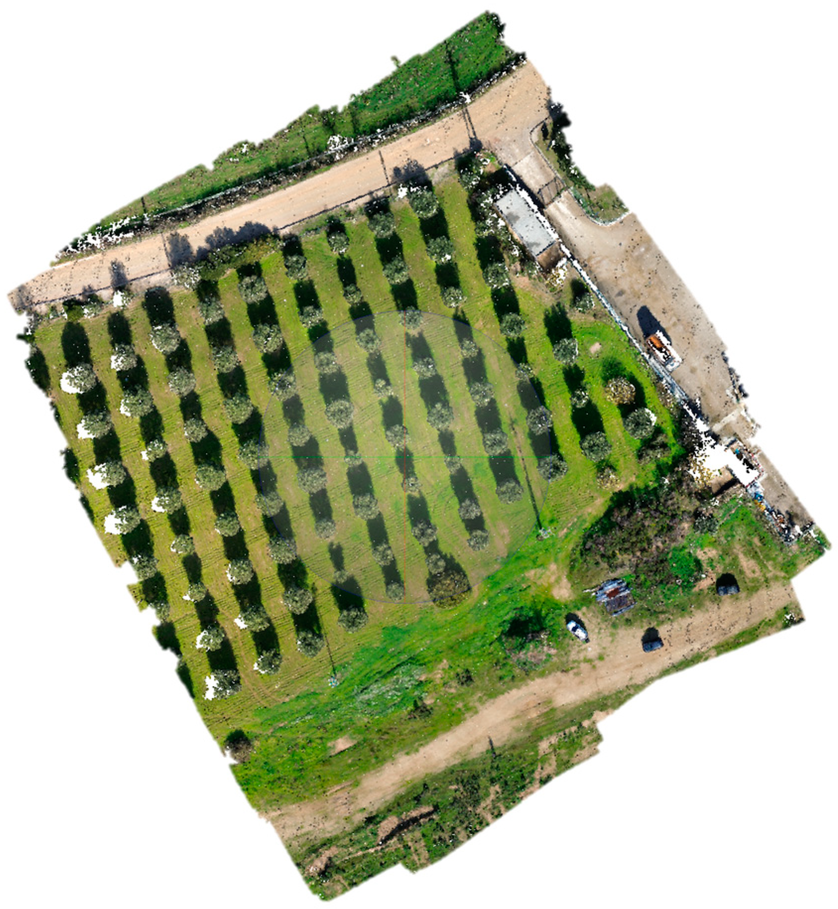
Two different study areas were chosen for the analysis, having different characteristics, especially in terms of mean tree height. The analysis aimed to test the possibility of applying the same method of height extraction in different conditions to evaluate possible limitations of the procedure. The first site, named “Area 1”, is part of an olive grove extended for about 1.2 hectares located in the South of Sardinia, Italy (Figure 1a). Approximately 80 olive trees cover the area following a precise configuration along separated rows, and the tree heights range between 3 m and 6 m (5 m on average). This area was chosen as the optimal case study for our application, considering the mean tree heights, the canopy extension, and the density of the foliage. The second site, hereafter called “Area 2”, consists of nearly 600 young trees placed along 26 rows with 2–3 m of inter-distance extending for about half a hectare (Figure 1b). Since the planting of the area was part of a requalification project that started a few months before the survey, here, the plants’ heights are generally very low, ranging between 10 cm and 140 cm and sometimes with leaf-off conditions. Moreover, the plantation in Area 2 involves three different plant species, having different typical characteristics in terms of foliage and mean heights: about 50 cm, 70 cm, and 85 cm for lentisk, poplar, and oleander, respectively. We want to stress that this second study area is particularly challenging due to the poor growth of the plants at the survey epoch.
2.2. UAV Photogrammetric Surveys
In Area 1, three UAV campaigns were performed using a very low-cost Mini 3—DJI drone equipped with an RGB sensor on the same day under the same weather conditions (Figure 2a). Three different flight altitudes were set, namely, 50 m, 40 m, and 30 m, for flights 1, 2, and 3, respectively. The flights were manually guided ensuring a resulting forward and side overlapping of 80% and 70%, respectively. A total of 6 GCPs were evenly distributed, 4 at the edges and 2 in the centre of the area. A good distribution of GCPs is of high importance not only for the image orientation but also for the prevention of block deformation effects that may result from the remaining systematic errors in the camera calibration [42,43]. The GCPs were surveyed using a single Trimble R8 GNSS receiver operating in NRTK mode for the georeferencing process. The GCP coordinates in terms of Northing and Easting aligned to the ETRF2000-UTM32N reference system (EPSG: 6707) were obtained exploiting the Sardinian SARNET network [44]. Moreover, ellipsoidal heights were converted into orthometric ones using ConveRgo software [45], which exploits the ITALGEO05 geoidheight grid (GK2 format) [46].
The UAV survey in Area 2, hereafter called “Flight a”, was carried out using a Phantom-DJI 4 drone equipped with RGB sensors and flying 42 m high. In this case, forward and side overlapping of 80% and 70%, respectively, were ensured through an automatic planning of the flight. The GCP survey followed the same method as the first site for a total of 7 points evenly distributed over the area, 4 at the corners and 3 in the centre (Figure 2b).
The GCPs were materialized on the ground using red and white circular targets with a diameter of 20 cm for both the surveyed sites (Figure 3). The shape and size of the targets were planned to be visible on images acquired flying up to 80 m high.
2.3. UAV Data Processing
Acquired images were processed using Agisoft Metashape software version 2.0.4 [47]. Metashape is a commercial software package widely used by the research community and by geomatics professionals to produce orthophotos, digital elevation models, and 3D models. Metashape implements the structure from motion (SfM) algorithm and multi-view stereo (MVS) techniques. The SfM algorithm allows fully automatic orientation of the images and reconstruction of a sparse model of the scene. The poses of the images, the spatial positions of the tracks, and the cameras’ calibration parameters were globally optimized with bundle block adjustment [48,49,50]. Moreover, Metashape software uses a hierarchical strategy for SfM reconstruction called HSfM, which is a natural extension of the incremental SfM (ISfM) [51]. MVS techniques were used to calculate the dense point cloud and to create three-dimensional models, serving as the base for the DSMs and orthophotos [38,52].
For each UAV dataset, we followed the workflow implemented in the software, consisting of the following steps: image import, image alignment, generation of the sparse point cloud, optimization of the image alignment, elaboration of the dense point cloud, and georeferencing. A total of 118, 86, 59, and 345 nadiral frames were acquired for Flights 1, 2, 3, and Flight “a”, respectively (Table 1), and all the images were aligned in the first step. The dense points clouds were processed by choosing high-quality parameters, which for Metashape software results in a preliminary downscaling of the image size by a factor of 4, 2 times by each side.
The dense point clouds were georeferenced using 6 GCPs for the flights of Area 1 and 7 GCPs for the flight of Area 2. The SD (standard deviation) and the minimum and maximum values of the georeferencing accuracies are reported in Table 3.
According to Table 3, high SD values related to Flight 3 in Area 1 are evident, and their possible sources were investigated. Although the analysis of the multiple GCPs on the images and their collimation did not result in any outcomes, we chose to use this dataset and verify its response to the methodology.
Table 4 reports the number of points in each point cloud and the size of the corresponding file; the dense point cloud of Flight 1 is shown in Figure 4 as an example.
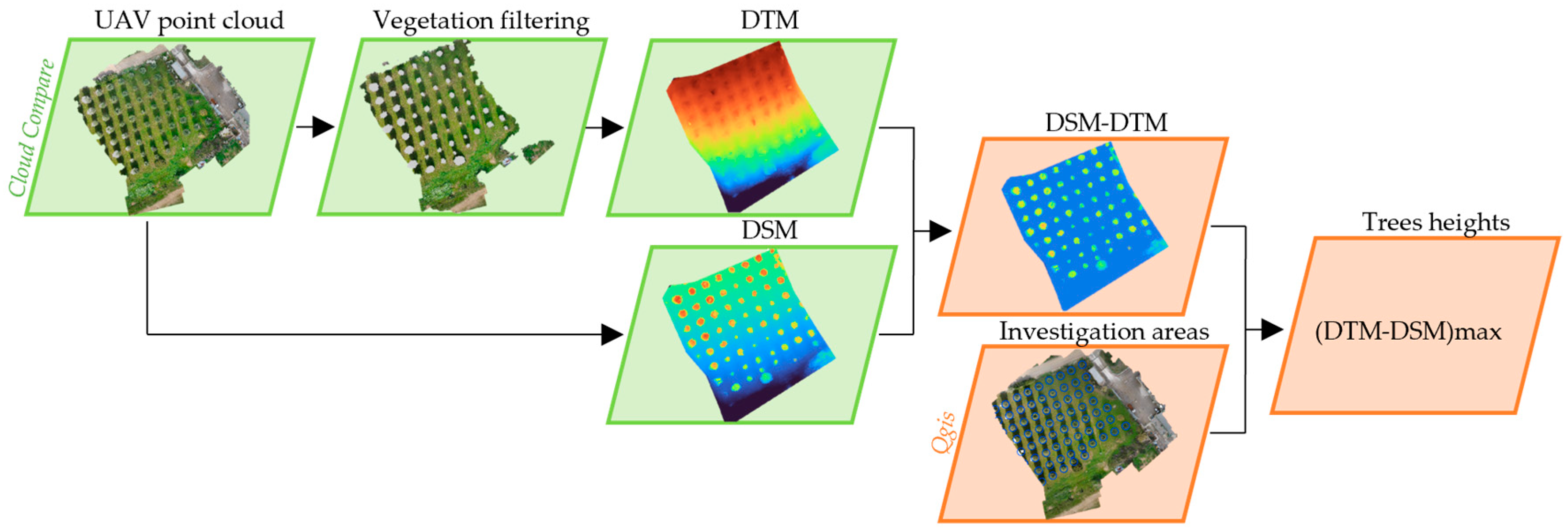
For each UAV survey, the dense point clouds were interpolated using the CloudCompare software package (version 2.12.14) [53] obtaining the corresponding DSM, with 20 cm of pixel dimension. Afterward, the applied methodology aimed at extracting the tree heights from the availability of a digital terrain model of the area provided by an external data source, using UAV-derived data to produce the reference DTM. This choice was possible also considering the negligible slope gradient of the terrain at both the chosen sites. Indeed, although CHMs originate from a normalization of the heights, minor terrain slopes ensure independent DTM processing without running into significant errors due to the interpolation process [10]. Nevertheless, bearing in mind the different characteristics between the two case studies in terms of tree heights and crown extensions, slightly different filtering procedures were used to produce the reference DTM. Indeed, Area 1 has mature olive trees with very defined canopies, while Area 2 includes at least small bushes. For this reason, the common automatic filtering operations, i.e., the inbuilt classification algorithms provided by the Agisoft Metashape and CloudCompare software, were not usable on the second site. In Area 1, the automatic filter implemented by CloudCompare software (Cloth Simulation Filter—CSF) was applied to split the UAV dense point clouds into “ground” and “off-ground” points. The following parameters were chosen for CSF processing: cloth resolution 1.0; max iterations 1000; and classification threshold 0.5. The vegetation filtering of the second dataset was manually carried out by exploiting the open-source LAStool package [54] implemented in Qgis software [55]. A clipping operation of the dense point cloud was performed, leading to the removal of the crowns from the original point cloud. After the filtering step, the DTMs of the two sites were generated by interpolating the ground points using the Rasterize tool in CloudCompare, choosing 20 cm of pixel dimension.
2.4. GIS-Based Approach for Tree Height Extraction
The maps of height variation have been computed as the differences between each DSM and the related DTM, using the Raster Calculator tool in Qgis software:
where the result represents the canopy height model (CHM) [33].
Finally, CHM maps were analysed in the GIS environment through a local maxima approach. In particular, the CHM values within trees’ individual neighbourhoods have been identified using the Zonal Statistic tool in Qgis software. This tool enables computing different statistics concerning the raster pixels included in selected regions. According to the local maxima approach, the maximums of the pixel retrieved values are the candidates to correspond to tree tops and thus can be selected as UAV-derived tree heights. Since both Area 1 and Area 2 have very defined plantation rows, there were no issues related to multiple matches of trees tops, which can happen for more structurally complex vegetation structures [56]. Therefore, maximum values were extracted and assigned to individual trees for the following analysis. Figure 5 graphically shows the complete workflow to extract the tree heights.
2.5. Field Measurements of Tree Heights and Statistical Analysis
All the UAV surveys were coupled with in-field measurements to be used for the validation process. In particular, the height of every single tree was directly measured using a metric rod. Field values were matched with the trees’ positions by exploiting a GIS-based procedure, obtaining a complete description of the area in terms of plant row, ID number, plant species (for Area 2), and plant height. Hereafter, we refer to these values as “field measurements”.
The accuracy of the tree height determination was assessed by computing different statistics. Residuals (r) showing the differences between each i-th UAV extracted height and the related field measurement collected in the field have been considered, as presented by Equation (2).
where hest and hmeas are the UAV heights and the measured ones, respectively. Minimum, maximum, mean, and standard deviation (SD) of the residuals were computed for each flight, together with values related to the 50% and 90% percentiles. Moreover, in order to represent the relationship between errors and related trees heights, the average value of the relative errors () was computed for each flight, following Equation (3).
where n is the number of trees.
Finally, the deviation between in-field values and extracted trees heights was provided through the root mean square error (RMSE), as shown in Equation (4).
The results are graphically presented using frequency distribution histograms of the residuals, and the relationship between the extracted and measured heights is reported in the form of scatter plots with linear regression lines. Indeed, the R2 parameters of each linear regression can be employed for the accuracy assessment. Furthermore, box and whisker plots were generated to have a graphical representation of the variances of both the estimated and measured trees heights.
3. Results
The main statistics of the residual values between extracted and measured heights for each flight are reported in Table 5.
Concerning Area 1, the results are within the expected method’s accuracy obtained for higher trees or in forestry contexts since the mean absolute values of the residuals range between 14 cm and 34 cm. As expected, the lower the flying altitude, i.e., the lower the GSD, the better coherence we found with the field measurements, from Flights 1 to 3. In particular, Flight 3 (30 m of flight altitude) shows very promising results, with 90% of the residuals below 50 cm. This result was also unexpected due to the high values of the RMSE related to the georeferencing process (Table 3). Nevertheless, a difference between the three flights arises since the former tend to underestimate the tree heights, while the third slightly overestimates their values (considering the field measurements as a reference in the comparison, as in Equation (2)). This fact is also evident from the frequency distribution histograms of the residuals in Figure 6a and should be further investigated to understand possible sources of this behaviour. Although Flight 3 involved a slightly smaller area compared with the previous ones, with a total of 41 identified trees, we can observe an almost normal distribution of the differences close to zero-centred. Finally, the relation between the residuals and the corresponding “real” height value (from the field measurement) has been analysed through the parameter. Very similar values are found for Flights 1 and 2, equal to 8.7% and 8.8%, respectively, whereas for Flight 3, is equal to 5.5%. These outcomes confirm the good results for the first site, meaning that the errors, i.e., the residuals in the height determination, are low compared to the absolute tree heights. This is further proved by the RMSE values, resulting in 0.47 m, 0.51 m, and 0.37 m, for Flights 1, 2, and 3, respectively.
The situation is different in Area 2, where Table 5 and Figure 6b show that values are entirely shifted toward the negatives, with a mean value of about minus 60 cm, i.e., nearly 30 cm more than the highest flight on Area 1 (Flight 1). This fact was expected from a first graphical inspection of the dense point cloud where plants were barely visible, mainly due to their very low heights, which affected the whole procedure. As a first aspect, independently of the following elaborations, it was difficult to obtain a good representation of shorter tree seedlings from the photogrammetric dense point cloud, considering the limited extension of the canopies and the foliage. Secondly, low heights negatively impact vegetation filtering, which cannot exploit automatic tools but rather requires a manual procedure. As a final point, comparing DSMs and DTMs, both of which derive from interpolation processes entraining sources of uncertainty, requires proper accuracies to enable small variations to be detected. Reasonably, these aspects mutually influence each other as well as the plant heights that are both the origin of the problem and the reason why the method is unusable in this context. Indeed, even if the field measurements are known to have accuracies lower than the cm-level, the obtained differences are comparable or sometimes higher than the actual tree heights in the area. Moreover, the same outcome is confirmed by the RMSE value, equal to 0.67 m.
Figure 7 shows the box and whisker plots of the estimated and measured tree heights for the three flights in Area 1. The minimum, maximum, and median values of the two datasets are highlighted, showing the higher variability in the estimated values compared to the measured ones as well as the underestimation trend for the first two flights, which is inverted in the case of Flight 3. Note that since the statistics related to the residuals already revealed the behaviour in Area 2, we decided not to show box charts for the second site.
The relationship between the estimated and measured tree heights for the three flights performed in Area 1 is presented in Figure 8. Looking at the linear regression lines, we can say that overall, the models, i.e., the estimated height values, are able to replicate the observed samples. Flight 1 and Flight 3 exhibit similar coefficients of determination (R2 = 0.67; R2 = 0.65), whereas the value is slightly lower for Flight 2 (R2 = 0.50). Similar considerations of the previous charts are made for Figure 8 relating to Area 2.
4. Discussion and Conclusions
To date, the monitoring and management of agricultural lands is a topic of high interest in the context of environmental protection and precision agriculture (PA), also due to the European Common Agricultural Policy (CAP) [57,58]. Indeed, there is a growing development in related research where geomatic surveys play a fundamental role.
This study focuses on the use of photogrammetric data to retrieve dimensional parameters of trees. The preliminary results of the tree height estimation from imagery acquired with low-cost UAV platforms are presented. The proposed methodology is based on photogrammetric processing exploiting the SfM technique, coupled with a GIS-based analysis. This analysis is straightforward and mainly based on open-source software, such as CloudCompare and Qgis, making again the whole procedure very flexible. Two study areas were chosen, named “Area 1” and “Area 2”, and a total of four UAV flights were performed. Starting from the UAV dense point clouds, the reference DTMs were produced by applying automatic filtering procedures or implementing a manual classification of ground and vegetation. The canopy height models obtained as differences between each DSM and the related DTM were analysed in the GIS environment using a local maxima approach choosing ad hoc regions as individual investigation areas around each tree. Thus, the candidate tree tops, corresponding to the maximum CHM pixel values, were identified and the related heights were considered in the analysis. The availability of in-field measurements concurrent with the UAV surveys supported the validation process and the statistical analysis, allowing for the method’s accuracy assessment.
In Area 1, the comparison with the field measurements provided promising results, with mean absolute residuals ranging between 14 and 34 cm. The best values are related to the campaign with 30 m of flying altitude, proving that the image resolution (GSD) is a fundamental parameter to obtain higher quality in the photogrammetric products. This fact is also supported by other studies, such as [22,29]. In particular, Pourreza et al. [29] used a DJI Phantom 4 flying at different altitudes (25 m, 50 m, and 100 m) over an area with tree heights comparable to ours, confirming that accuracy is negatively dependent on the flight altitudes. Moreover, all the flights in Area 1 exhibit 50% of the residuals lower than 38 cm, and the frequency distribution histograms of the residuals follow almost normal distributions. Results in the first site are also coherent with the outcomes of a similar study by Zarco-Tejada et al. [28], where they obtained an RMSE of 35 cm for tree heights ranging between 1.16 m and 4.38 m. Concerning the coefficients of determination related to the tree height estimation, their higher value (R2 = 0.83 versus our R2 = 0.67) could be related to the difference in the field measurements used for the validation. Indeed, we are aware that the use of a metric rod inevitably suffers from the weather conditions, in particular the wind, the tree characteristics in terms of foliage and the crown’s extension and the subjective nature affecting the observations. Birdal et al. [26] found an RMSE equal to 28 cm for trees ranging between 1.2 m and 7.1 m, which is also consistent with our findings, whereas their R2 parameter is significantly higher (0.95). Similar results can be found in [14,21,23,31], whose findings outline RMSE and R2 values comparable to ours in contexts of higher trees. However, results of the different flights in the first site exhibit different behaviours, since Flights 1 and 2 generally underestimate the trees’ heights, while Flight 3 tends to overestimate. Since results of other studies generally confirm the underestimation trend of UAV extracted heights [21,29], this fact requires further investigation, which will be developed in future studies.
As expected, the context in Area 2 entailed different conclusions since the mean value of the residuals is about −60 cm, i.e., sometimes higher than the actual tree heights in the area. Even if the flight altitude was comparable with the one of Flight 1, the mean value of the residuals is 30 cm higher. This fact is reasonably not only due to the altitude rather than to the “absolute” height of the individual trees that made the whole procedure very challenging. Indeed, we want again to stress the complexity of the context chosen in the case of Area 2, where tree heights are always below 1.5 m and the foliage is poorly grown. We identified three main aspects impacting this outcome: (i) goodness of the photogrammetric dense cloud in representing shorter tree seedlings; (ii) manual vegetation filtering; and (iii) impact of the interpolation in the DSM and DTM generation and differencing. Although the obtained results make the methodology not usable for this range of heights, bearing in mind the presence of different plant species in Area 2, we tried to relate the results with this parameter. However, no evidence has arisen, unless a slightly better behaviour of the lentisk compared with the other two species (poplar, oleander), but probably reliable results would require higher plants to allow their differentiation by foliage and crown extensions.
Overall, the obtained results confirm the suitability of UAV photogrammetric data acquired from low-cost instruments for tree height extraction. The implementation of the same procedure to multitemporal datasets acquired at low-flight altitudes could allow even the determination of the rate of growth of trees over medium–long temporal scales. These become key data in the analysis of phytoremediation processes when assessing the plant’s health and the effectiveness of the chosen restoration method. Moreover, since the usage of low-cost UAV equipment is easily accessible even for non-specialist users, the possibility of easily adopting the same workflow represents a benefit for all those involved in the agricultural field. Nevertheless, the application of the same methodology in the context of shorter tree seedlings requires further investigation, and possible future development of this research may involve UAV campaigns at lower flying altitudes and an intermediate case study of Area 2 after the plants’ growth.
Finally, it should be highlighted that this research is framed in the context of a wider project, “Tecnologie di CARatterizzazione Monitoraggio e Analisi per il ripristino e la bonifica (CARMA)”, involving both geomatics and geophysical data [59]. Thus, the presented study is the first step to reaching the project’s goals of integrating geometric, biochemical, and geophysical data in a single workflow to assess tree health and rates of growth. Considering this multidisciplinary context, future developments may involve the employment of more advanced technologies, such as LiDAR, to improve the accuracy, especially in areas with shorter tree seedlings. In addition, future analysis will exploit both nadiral and oblique images, as suggested in [26,29]. Indeed, the use of oblique images leads to improvements in the final accuracy since they allow the point cloud to better capture the ground points under and around trees, resulting in enhanced classification processes.
Author Contributions
Conceptualization, G.V. and E.V.; methodology, G.V. and E.V.; software, E.V.; resources, G.V.; writing—review and editing, E.V. and G.V.; and supervision, G.V. All authors have read and agreed to the published version of the manuscript.
Funding
This research was funded by Sardegna Ricerca, CUP: G28C17000250006, https://www.ecoserdiana.com/servizi/progetti-di-ricerca.html (accessed on 5 January 2024).
Data Availability Statement
The raw data supporting the conclusions of this article will be made available by the authors on request.
Acknowledgments
The authors are grateful to Pasquale Carta, Andrea Dessì, Sergio De Montis, and Federico Secchi for their contribution during the field surveys.
Conflicts of Interest
The authors declare no conflicts of interest.
References
- Ammoniaci, M.; Kartsiotis, S.-P.; Perria, R.; Storchi, P. State of the Art of Monitoring Technologies and Data Processing for Precision Viticulture. Agriculture 2021, 11, 201. [Google Scholar] [CrossRef]
- Pagliai, A.; Ammoniaci, M.; Sarri, D.; Lisci, R.; Perria, R.; Vieri, M.; D’Arcangelo, M.E.M.; Storchi, P.; Kartsiotis, S.-P. Comparison of Aerial and Ground 3D Point Clouds for Canopy Size Assessment in Precision Viticulture. Remote Sens. 2022, 14, 1145. [Google Scholar] [CrossRef]
- Crookston, R.K. A top 10 list of developments and issue impacting crop management and ecology during the past 50 years. Crop Sci. 2006, 46, 2253–2262. [Google Scholar] [CrossRef]
- Casa, R.; Airoldi, G.; Balsari, P.; Basso, B.; Boschetti, M.; Buttafuoco, G.; Calcante, A.; Cammarano, D.; Castaldi, F.; Castrignanò, A.; et al. Agricoltura diprecisione. Metodi etecnologie per migliorare l’efficienza e lasostenibilità dei sistemi colturali. In Agricoltura di Precisione; Edagricole—Edizioni Agricole di New Business Media srl: Milano, Italy, 2016; Available online: https://www.edagricole.it/wp-content/uploads/2020/03/5510-Agricoltura-di-precisione-SFOGLIA.pdf (accessed on 1 September 2023).
- Vacca, G.; Quaquero, E. BIM-3D GIS: An integrated system for the knowledge process of the buildings. J. Spat. Sci. 2020, 65, 193–208. [Google Scholar] [CrossRef]
- Belcore, E.; Angeli, S.; Colucci, E.; Musci, M.A.; Aicardi, I. Precision Agriculture Workflow, from Data Collection to Data Management Using FOSS Tools: An Application in Northern Italy Vineyard. ISPRS Int. J. Geo-Inf. 2021, 10, 236. [Google Scholar] [CrossRef]
- Hobart, M.; Pflanz, M.; Weltzien, C.; Schirrmann, M. Growth height determination of tree walls for precise monitoring in apple fruit production using UAV photogrammetry. Remote Sens. 2020, 12, 1656. [Google Scholar] [CrossRef]
- Zaru, N.; Rossi, M.; Vacca, G.; Vignoli, G. Spreading of Localized Information across an Entire 3D Electrical Resistivity Volume via Constrained EMI Inversion Based on a Realistic Prior Distribution. Remote Sens. 2022, 15, 3993. [Google Scholar] [CrossRef]
- Gonzalez-Dugo, V.; Zarco-Tejada, P.; Nicolás, E.; Nortes, P.A.; Alarcón, J.J.; Intrigliolo, D.S.; Fereres, E. Using high-resolution UAV thermal imagery to assess the variability in the water status of five fruit tree species within a commercial orchard. Precis. Agric. 2013, 14, 660–678. [Google Scholar] [CrossRef]
- Vecchi, E.; Tavasci, L.; De Nigris, N.; Gandolfi, S. GNSS and photogrammetric UAV derived data for coastal monitoring: A case of study in Emilia-Romagna, Italy. J. Mar. Sci. Eng. 2021, 9, 1194. [Google Scholar] [CrossRef]
- Zhang, H.L.; Tian, W.T.; Yin, J. A Review of Unmanned Aerial Vehicle Low-Altitude Remote Sensing (UAV-LARS) Use in Agricultural Monitoring in China. Remote Sens. 2021, 13, 1221. [Google Scholar] [CrossRef]
- Remondino, F.; Barazzetti, L.; Nex, F.; Scaioni, M.; Sarazzi, D. UAV photogrammetry for mapping and 3d modelling–current status and future perspectives. Int. Arch. Photogramm. Remote Sens. Spat. Inf. Sci. 2012, 38, 25–31. [Google Scholar] [CrossRef]
- Wallace, L. Assessing the stability of canopy maps produced from UAV-LiDAR data. In Proceedings of the IEEE International Geoscience and Remote Sensing Symposium-IGARSS, Melbourne, Australia, 21–26 July 2013; pp. 3879–3882. [Google Scholar]
- Wallace, L.; Lucieer, A.; Malenovský, Z.; Turner, D.; Vopěnka, P. Assessment of forest structure using two UAV techniques: A comparison of airborne laser scanning and structure from motion (SfM) point clouds. Forests 2016, 7, 62. [Google Scholar] [CrossRef]
- Argamosa, R.J.L.; Paringit, E.C.; Quinton, K.R.; Tandoc, F.A.M.; Faelga, R.A.G.; Ibañez, C.A.G.; Posilero, M.A.V.; Zaragosa, G.P. Fully automated GIS-based individual tree crown delineation based on curvature values from a lidar derived canopy height model in a coniferous plantation. Int. Arch. Photogramm Remote Sens. Spat. Inf. Sci. 2016, 41, 563–569. [Google Scholar] [CrossRef]
- Beloiu, M.; Heinzmann, L.; Rehush, N.; Gessler, A.; Griess, V.C. Individual Tree-Crown Detection and Species Identification in Heterogeneous Forests Using Aerial RGB Imagery and Deep Learning. Remote Sens. 2023, 15, 1463. [Google Scholar] [CrossRef]
- Tiede, D.; Hochleitner, G.; Blaschke, T. A full GIS-based workflow for tree identification and tree crown delineation using laser scanning. In Proceedings of the ISPRS Workshop CMRT 2005, Vienna, Australia, 29–30 August 2005; Volume 5. [Google Scholar]
- Latella, M.; Sola, F.; Camporeale, C. A density-based algorithm for the detection of individual trees from LiDAR data. Remote Sens. 2021, 13, 322. [Google Scholar] [CrossRef]
- Velusamy, P.; Rajendran, S.; Mahendran, R.K.; Naseer, S.; Shafiq, M.; Choi, J.-G. Unmanned Aerial Vehicles (UAV) in Precision Agriculture: Applications and Challenges. Energies 2022, 15, 217. [Google Scholar] [CrossRef]
- Panagiotidis, D.; Abdollahnejad, A.; Slavik, M. 3D point cloud fusion from UAV and TLS to assess temperate managed forest structures. Int. J. Appl. Earth Obs. Geoinf. 2022, 112, 102917. [Google Scholar] [CrossRef]
- Krause, S.; Sanders, T.G.; Mund, J.P.; Greve, K. UAV-based photogrammetric tree height measurement for intensive forest monitoring. Remote Sens. 2019, 11, 758. [Google Scholar] [CrossRef]
- Kameyama, S.; Sugiura, K. Estimating tree height and volume using unmanned aerial vehicle photography and SfM technology, with verification of result accuracy. Drones 2020, 4, 19. [Google Scholar] [CrossRef]
- Yurtseven, H.; Akgul, M.; Coban, S.; Gulci, S. Determination and accuracy analysis of individual tree crown parameters using UAV based imagery and OBIA techniques. Measurement 2019, 145, 651–664. [Google Scholar] [CrossRef]
- Komárek, J.; Klápště, P.; Hrach, K.; Klouček, T. The potential of widespread UAV cameras in the identification of conifers and the delineation of their crowns. Forests 2022, 13, 710. [Google Scholar] [CrossRef]
- Huo, L.; Lindberg, E.; Holmgren, J. Towards low vegetation identification: A new method for tree crown segmentation from LiDAR data based on a symmetrical structure detection algorithm (SSD). Remote Sens. Environ. 2022, 270, 112857. [Google Scholar] [CrossRef]
- Birdal, A.C.; Avdan, U.; Türk, T. Estimating tree heights with images from an unmanned aerial vehicle. Geomat. Nat. Hazards Risk 2017, 8, 1144–1156. [Google Scholar] [CrossRef]
- Moudrý, V.; Klápště, P.; Fogl, M.; Gdulová, K.; Barták, V.; Urban, R. Assessment of LiDAR ground filtering algorithms for determining ground surface of non-natural terrain overgrown with forest and steppe vegetation. Measurement 2020, 150, 107047. [Google Scholar] [CrossRef]
- Zarco-Tejada, P.J.; Diaz-Varela, R.; Angileri, V.; Loudjani, P. Tree height quantification using very high resolution imagery acquired from an unmanned aerial vehicle (UAV) and automatic 3D photo-reconstruction methods. Eur. J. Agron. 2014, 55, 89–99. [Google Scholar] [CrossRef]
- Pourreza, M.; Moradi, F.; Khosravi, M.; Deljouei, A.; Vanderhoof, M.K. GCPs-free photogrammetry for estimating tree height and crown diameter in Arizona Cypress plantation using UAV-mounted GNSS RTK. Forests 2022, 13, 1905. [Google Scholar] [CrossRef]
- Surový, P.; Ribeiro, N.A.; Panagiotidis, D. Estimation of positions and heights from UAV-sensed imagery in tree plantations in agrosilvopastoral systems. Int. J. Remote Sens. 2018, 39, 4786–4800. [Google Scholar] [CrossRef]
- Gülci, S. The determination of some stand parameters using SfM-based spatial 3D point cloud in forestry studies: An analysis of data production in pure coniferous young forest stands. Environ. Monit. Assess. 2019, 191, 495. [Google Scholar] [CrossRef]
- Lisein, J.; Pierrot-Deseilligny, M.; Bonnet, S.; Lejeune, P. A photogrammetric workflow for the creation of a forest canopy height model from small unmanned aerial system imagery. Forests 2013, 4, 922–944. [Google Scholar] [CrossRef]
- Mohan, M.; Silva, C.A.; Klauberg, C.; Jat, P.; Catts, G.; Cardil, A.; Hudak, A.T.; Dia, M. Individual Tree Detection from Unmanned Aerial Vehicle (UAV) Derived Canopy Height Model in an Open Canopy Mixed Conifer Forest. Forests 2017, 8, 340. [Google Scholar] [CrossRef]
- Pearse, G.D.; Dash, J.P.; Persson, H.J.; Watt, M.S. Comparison of high-density LiDAR and satellite photogrammetry for forest inventory. ISPRS J. Photogramm. Remote Sens. 2018, 142, 257–267. [Google Scholar] [CrossRef]
- Belcore, E.; Latella, M. Riparian ecosystems mapping at fine scale: A density approach based on multi-temporal UAV photogrammetric point clouds. Remote Sens. Ecol. Conserv. 2022, 8, 644–655. [Google Scholar] [CrossRef]
- Dandois, J.P.; Ellis, E.C. High spatial resolution three-dimensional mapping of vegetation spectral dynamics using computer vision. Remote Sens. Environ. 2013, 136, 259–276. [Google Scholar] [CrossRef]
- Popescu, S.C. Estimating biomass of individual pine trees using airborne lidar. Biomass Bioenergy 2007, 31, 646–655. [Google Scholar] [CrossRef]
- Vacca, G. Estimating tree height using low-cost UAV. Int. Arch. Photogramm. Remote Sens. Spatial Inf. Sci. 2023, 48, 381–386. [Google Scholar] [CrossRef]
- Naveed, M.; Ghaffar, M.; Khan, Z.; Gul, N.; Ijaz, I.; Bibi, A.; Pervaiz, S.; Alharby, H.F.; Tariq, M.S.; Ahmed, S.R.; et al. Morphological and Structural Responses of Albizia lebbeck to Different Lead and Nickel Stress Levels. Agriculture 2023, 13, 1302. [Google Scholar] [CrossRef]
- Wang, Y.; Wang, S.; Zhao, Z.; Zhang, K.; Tian, C.; Mai, W. Progress of Euhalophyte Adaptation to Arid Areas to Remediate Salinized Soil. Agriculture 2023, 13, 704. [Google Scholar] [CrossRef]
- Matsuura, Y.; Heming, Z.; Nakao, K.; Qiong, C.; Firmansyah, I.; Kawai, S.; Yamaguchi, Y.; Maruyama, T.; Hayashi, H.; Nobuhara, H. High-precision plant height measurement by drone with RTK-GNSS and single camera for real-time processing. Sci. Rep. 2023, 13, 6329. [Google Scholar] [CrossRef]
- Shahbazi, M.; Sohn, G.; Théau, J.; Menard, P. Development and Evaluation of a UAV-Photogrammetry System for Precise 3D Environmental Modeling. Sensors 2015, 15, 27493–27524. [Google Scholar] [CrossRef]
- Sanz-Ablanedo, E.; Chandler, J.H.; Rodríguez-Pérez, J.R.; Ordóñez, C. Accuracy of Unmanned Aerial Vehicle (UAV) and SfM Photogrammetry Survey as a Function of the Number and Location of Ground Control Points Used. Remote Sens. 2018, 10, 1606. [Google Scholar] [CrossRef]
- Sarnet, Web Server della Rete di Stazioni Permanenti Della Sardegna. Available online: www.sarnet.it/servizi.html (accessed on 1 January 2024).
- Centro Interregionale per I Sistemi Informatici Geografici e Statistici In Liquidazione. Trasformazioni di Coordinate—Il Software ConveRgo. Available online: https://www.cisis.it/?page_id=3214 (accessed on 1 January 2024).
- International Service for the Geoid (ISG). Italy (ITALGEO05). Available online: https://www.isgeoid.polimi.it/Geoid/Europe/Italy/italgeo05_g.html (accessed on 1 January 2024).
- AgiSoft PhotoScan Standard (Version 1.2.6) (Software). (2016*). Available online: http://www.agisoft.com/downloads/installer/ (accessed on 27 January 2024).
- Turner, D.; Lucieer, A.; Watson, C. An automated technique for generating georectified mosaics from ultra-high resolution unmanned aerial vehicle (UAV) imagery, based on structure from motion (SfM) point clouds. Remote Sens. 2012, 4, 1392–1410. [Google Scholar] [CrossRef]
- Szeliski, R. Computer Vision: Algorithms and Applications; Springer Nature: Berlin/Heidelberg, Germany, 2022. [Google Scholar]
- Jiang, S.; Jiang, C.; Jiang, W. Efficient structure from motion for large-scale UAV images: A review and a comparison of SfM tools. ISPRS J. Photogramm. Remote Sens. 2020, 167, 230–251. [Google Scholar] [CrossRef]
- Liang, Y.; Yang, Y.; Fan, X.; Cui, T. Efficient and Accurate Hierarchical SfM Based on Adaptive Track Selection for Large-Scale Oblique Images. Remote Sens. 2023, 15, 1374. [Google Scholar] [CrossRef]
- Lingua, A.M.; Maschio, P.; Spadaro, A.; Vezza, P.; Negro, G. Iterative Refraction-Correction Method on Mvs-Sfm for Shallow Stream Bathymetry. Int. Arch. Photogramm. Remote Sens. Spat. Inf. Sci. 2023, XLVIII-1/W1-2023, 249–255. [Google Scholar] [CrossRef]
- CloudCompare. Available online: https://www.danielgm.net/cc/ (accessed on 1 January 2024).
- Isenburg, M. LAStools—Efficient LiDAR Processing Software (Version 141017, Unlicensed). Available online: http://rapidlasso.com/LAStools (accessed on 1 September 2023).
- Qgis Documentation. Available online: https://docs.qgis.org/2.8/en/ (accessed on 1 January 2024).
- Panagiotidis, D.; Abdollahnejad, A.; Surový, P.; Chiteculo, V. Determining tree height and crown diameter from high-resolution UAV imagery. Int. J. Remote Sens. 2017, 38, 2392–2410. [Google Scholar] [CrossRef]
- European Commission. Agriculture and Rural Development, Common Agricultural Policy. Available online: https://agriculture.ec.europa.eu/common-agricultural-policy_en#:~:text=The%20CAP%20is%20a%20partnership,27%20commenced%201%20January%202023 (accessed on 1 January 2024).
- Alexandratos, N.; Bruinsma, J. World Agriculture towards 2030/2050: The 2012 Revision; ESA Working Paper 2012 12-03; FAO: Rome, Italy, 2012. [Google Scholar]
- Ecoserdiana. Progetto di Ricerca su Tecnologie di CARatterizzazione Monitoraggio e Analisi per il Ripristino e la Bonifica (CARMA)—Fondo Europeo di Sviluppo Regionale—Por Fesr Sardegna 2014–2020. Available online: https://www.ecoserdiana.com/servizi/progetti-di-ricerca.html (accessed on 1 December 2023).
Figure 1.
National and local contextualization of the study areas located in the South of Sardinia, Italy. (a) refers to Area 1 (olive grove site); (b) refers to Area 2 (plantation of poplar, lentisk, and oleander). Basemap: Google Satellite. The map was generated using Qgis software (version 3.28.15) and the coordinates are aligned to the ETRS89-ETRF2000-UTM32 reference system (EPSG: 6707).

Figure 2.
Tree rows and UAV campaigns in the study areas: (a) refers to Area 1; (b) refers to Area 2, during the GNSS-NRTK survey of the GCPs.
Figure 2.
Tree rows and UAV campaigns in the study areas: (a) refers to Area 1; (b) refers to Area 2, during the GNSS-NRTK survey of the GCPs.

Figure 3.
Example of a circular target used as a ground control point (GCP).

Figure 4.
Dense point cloud of Flight 1 (Area 1).

Figure 5.
Schematic representation of the workflow for tree height extraction.

Figure 6.
Frequency distribution histograms of the residuals between the extracted and measured tree heights: (a) Area 1—Flights 1, 2, and 3; (b) Area 2—Flight a.
Figure 6.
Frequency distribution histograms of the residuals between the extracted and measured tree heights: (a) Area 1—Flights 1, 2, and 3; (b) Area 2—Flight a.

Figure 7.
Box and whisker plots showing the variance of the measured and estimated tree heights for the three flights in Area 1.
Figure 7.
Box and whisker plots showing the variance of the measured and estimated tree heights for the three flights in Area 1.

Figure 8.
Relationship between estimated and measured tree heights, linear regression, and related parameters for the three UAV campaigns in Area 1.
Figure 8.
Relationship between estimated and measured tree heights, linear regression, and related parameters for the three UAV campaigns in Area 1.


Table 1.
Summary of the UAV flight parameters for Area 1 and Area 2.
| Site | Flight Name | Date and Time of the Survey | Flying Altitude (m) | Flight Path Pattern | GSD | n GCPs | n Frames (Nadiral) |
|---|---|---|---|---|---|---|---|
| Area 1 | 1 | 14 December 2023 From 11:13:49 to 11:28:22 | 50 | North-South | 1.61 cm/pix | 6 | 118 |
| 2 | 14 December 2023 From 11:34:23 to 11:43:51 | 40 | North-South | 1.14 cm/pix | 6 | 86 | |
| 3 | 14 December 2023 From 11:49:56 to 11:55:42 | 30 | North-South | 0.53 cm/pix | 6 | 59 | |
| Area 2 | a | 3 January 2023 From 10:01:22 to 10:15:22 | 42 | NE-SW | 1.07 cm/pix | 7 | 345 |
Table 2.
Camera parameters.
| Site | Sensor Size (Pixels) | Focal Length (mm) Full-Frame Equivalent | Pixel Size on the Sensor (µm) |
|---|---|---|---|
| Area 1 | 12 MP | 24 | 2.64 |
| Area 2 | 12.4 MP | 20 | 2.41 |
Table 3.
Standard deviation (SD), minimum and maximum values of the georeferencing accuracy. Values are expressed in centimetres.
Table 3.
Standard deviation (SD), minimum and maximum values of the georeferencing accuracy. Values are expressed in centimetres.
| Site | Flight Name | n GCPs | SD (cm) (X; Y; Z) | Min; Max Accuracy (cm) X | Min; Max Accuracy (cm) Y | Min; Max Accuracy (cm) Z |
|---|---|---|---|---|---|---|
| Area 1 | 1 | 6 | 1.4; 2.8; 2.3 | −1.2; 2.4 | 0.3; 5.4 | −3.3; 2.9 |
| 2 | 6 | 0.9; 2.5; 6.5 | −0.4; 1.6 | −3.8; 2.8 | −8.5; 1.6 | |
| 3 | 6 | 6.1; 7.9; 7.2 | −9.5; 2.8 | −3.0; 13.3 | −3.0; 11.3 | |
| Area 2 | a | 7 | 1.8; 0.8; 2.2 | −1.8; 4.0 | −1.3; 1.1 | −1.7; 2.2 |
Table 4.
Point cloud characteristics in terms of number of points and file size.
| Site | Flight | N Points | File Size |
|---|---|---|---|
| Area 1 | 1 | 82 million | 2.30 GB |
| 2 | 104 million | 2.52 GB | |
| 3 | 95 million | 2.31 GB | |
| Area 2 | a | 105 million | 2.55 GB |
Table 5.
Residuals between estimated tree heights and measured values: minimum, maximum and mean values, standard deviations, and 50% and 90% percentiles are given for each flight. Values are expressed in metres.
Table 5.
Residuals between estimated tree heights and measured values: minimum, maximum and mean values, standard deviations, and 50% and 90% percentiles are given for each flight. Values are expressed in metres.
| Site | Flight | Min (m) | Max (m) | Mean (m) | SD (m) | 50%ile (m) | 90%ile (m) |
|---|---|---|---|---|---|---|---|
| Area 1 | 1 | −1.13 | 0.70 | −0.34 | 0.34 | 0.38 | 0.72 |
| 2 | −1.30 | 1.37 | −0.26 | 0.44 | 0.31 | 0.87 | |
| 3 | −0.42 | 1.46 | 0.14 | 0.28 | 0.16 | 0.49 | |
| Area 2 | a | −1.37 | −0.04 | −0.62 | 0.24 | 0.57 | 0.96 |
Disclaimer/Publisher’s Note: The statements, opinions and data contained in all publications are solely those of the individual author(s) and contributor(s) and not of MDPI and/or the editor(s). MDPI and/or the editor(s) disclaim responsibility for any injury to people or property resulting from any ideas, methods, instructions or products referred to in the content. |
© 2024 by the authors. Licensee MDPI, Basel, Switzerland. This article is an open access article distributed under the terms and conditions of the Creative Commons Attribution (CC BY) license (https://creativecommons.org/licenses/by/4.0/).
Share and Cite
MDPI and ACS Style
Vacca, G.; Vecchi, E. UAV Photogrammetric Surveys for Tree Height Estimation. Drones 2024, 8, 106. https://doi.org/10.3390/drones8030106
AMA Style
Vacca G, Vecchi E. UAV Photogrammetric Surveys for Tree Height Estimation. Drones. 2024; 8(3):106. https://doi.org/10.3390/drones8030106
Chicago/Turabian StyleVacca, Giuseppina, and Enrica Vecchi. 2024. "UAV Photogrammetric Surveys for Tree Height Estimation" Drones 8, no. 3: 106. https://doi.org/10.3390/drones8030106