
Saturated Trajectory Tracking Controller in the Body-Frame for Quadrotors
by
 , , , and
João Madeiras
1,*,
Carlos Cardeira
1,
Paulo Oliveira
1,2,
Pedro Batista
2 and
Carlos Silvestre
2,3 1
IDMEC —Institute of Mechanical Engineering, Instituto Superior Técnico, Universidade de Lisboa, 1049-001 Lisboa, Portugal
2
ISR—Institute for Systems and Robotics, Instituto Superior Técnico, Universidade de Lisboa, 1049-001 Lisboa, Portugal
3
Department of Electrical and Computer Engineering, Faculty of Science and Technology, University of Macau, Macao 999078, China
*
Author to whom correspondence should be addressed.
Drones 2024, 8(4), 163; https://doi.org/10.3390/drones8040163
Submission received: 26 February 2024
/
Revised: 30 March 2024
/
Accepted: 16 April 2024
/
Published: 19 April 2024
(This article belongs to the Section Drone Design and Development)
Abstract
:This paper introduces a quadrotor trajectory tracking controller comprising a steady-state optimal position controller with a normed input saturation and modular integrative action coupled with a backstepping attitude controller. First, the translational and rotational dynamical models are designed in the body-fixed frame to avoid external rotations and are partitioned into an underactuated position system and a quaternion-based attitude system. Secondly, a controller is designed separately for each subsystem, namely, (i) the position controller synthesis is derived from the Maximum Principle, Lyapunov, and linear quadratic regulator (LQR) theory, ensuring the global exponential stability and steady-state optimality of the controller within the linear region, and global asymptotic stability is guaranteed for the saturation region when coupled with any local exponential stable attitude controller, and (ii) the attitude system, with the quaternion angles and the angular velocity as the controlled variables, is designed in the error space through the backstepping technique, which renders the overall system, position, and attitude, with desirable closed-loop properties that are almost global. The overall stability of the system is achieved through the propagation of the position interconnection term to the attitude system. To enhance the robustness of the tracking system, integrative action is devised for both position and attitude, with emphasis on the modular approach for the integrative action on the position controller. The proposed method is experimentally validated on board an off-the-shelf quadrotor to assess the resulting performance.
1. Introduction
In recent years, quadrotors have emerged as versatile aerial platforms, with applications spanning from surveillance and inspection to aerial photography and autonomous exploration. The inherent agility and maneuverability of these vehicles have rendered them indispensable in various fields [1,2]. To fully exploit the capabilities of quadrotors in tracking tasks, precise and robust control strategies are paramount. The trajectory tracking problem for quadrotors is challenging due to their nonlinear dynamics and underactuated nature, and many control strategies have been devised [2,3].
With the purpose of taking the maximum benefit of the capabilities of these vehicles for tracking purposes, numerous controllers have been proposed [4,5,6]. In [7], successful implementation of linear control techniques, including the linear quadratic regulator (LQR), was achieved for low-speed indoor flights. However, these linear techniques often rely on the linearization of quadcopter dynamics, which can limit their ability to fully explore the vehicle’s flight envelope and establish a clear region of attraction for stability. In the literature, various nonlinear approaches are available, including feedback linearization [8], backstepping [9], differential flatness [10], and sliding mode control.
Nowadays, state-of-the-art research in quadrotor control blends hierarchical control with geometric feedback. This method entails the creation of a virtual feedback law at the acceleration level, which is subsequently extended to the inner attitude controller. A geometric approach for trajectory tracking with thrust vectoring capabilities is proposed in [11], where position tracking can be achieved by easing attitude tracking requirements. Asymptotic stability is proved for the entire system. In [12], the stability of the system is tackled through integral input-to-state stability. This method yields a quasi-time-optimal control law, which achieves global asymptotic stabilization for any initial position. As a result, it enhances transient performance compared with existing control designs. Recent significant contributions to quadrotor control, which combine hierarchical control with geometric feedback, can be found in [13,14,15,16].
The backstepping method has been extensively applied in various studies to control underactuated quadrotors, as documented in [17,18,19]. In these approaches, the attitude error is skillfully derived either from the error in the thrust direction or through traditional backstepping techniques. This results in the interconnection term being backstepped into the attitude control law, effectively canceling its influence.
In the field of quadrotor control, effectively handling system dynamics within the constraints of actuator limits is of paramount importance. The intrinsic underactuated nature of quadrotors necessitates sophisticated control strategies that can handle the nonlinear constraints imposed by actuator saturation. The formulation of control laws incorporating saturation for quadrotors typically aims to avert the singularity linked with a null thrust value, thereby ensuring well-posed attitude references [14,16,20]. This approach is critical, as it ensures that the system remains robustly stable and bounded, regardless of the given trajectory. Moreover, such control laws can provide large regions of attraction with disturbances rejection capability in a closed-form solution [21]. A recently emerging alternative strategy is the Explicit Reference Governor (ERG), which has gained traction in the field. This Lyapunov-based scheme acts as an add-on to prestabilized systems, from which the reference commands are modified to ensure the handling of constraints [22]. The ERG closed-form solutions are particularly advantageous for constraint applications with limited computational resources but may lead to conservative solutions [23]. This method has been successfully applied to underactuated Unnamed Air Vehicles (UAVs), demonstrating its efficacy in real-time constraint management [24,25].
This work presents a quadrotor trajectory tracking controller that integrates a steady-state optimal position controller with normed saturated input and a backstepping attitude controller. This approach is characterized by a blend of inner–outer loop theory and backstepping, enhancing transient performance. The dynamical models for translation and rotation are designed in the body-fixed frame to prevent external rotations (algebraic transformations to convert sensor data into inertial coordinates) and are split into underactuated position and quaternion-based attitude systems. Separate controllers are crafted for each subsystem. The position controller is synthesized with a modular integrative action using the Maximum Principle, Lyapunov, and linear quadratic regulator theory, ensuring global exponential stability and steady-state optimality in the linear region, with global asymptotic stability (GAS) guaranteed in the saturation region. On the other hand, the attitude system, with quaternion angles and angular velocity as controlled variables, is developed using the backstepping technique, ensuring desirable almost global closed-loop properties as a consequence of the double cover quaternion representation [26]. The position controllers are designed with a normed input saturation with the shown GAS property when coupled with any attitude controller with local exponential stability. This strategic approach ensures stability throughout the operation, preserving both GAS and local exponential stability for the overall system.
The proposed methodology incorporates rigid-body translational dynamics expressed in body-fixed coordinates, which is rooted in several compelling benefits. One of the notable advantages is the avoidance of algebraic transformations to convert sensor data into inertial coordinates. This avoidance is crucial as it helps minimize the amplification of noise and biases on attitude estimates, a viewpoint highlighted in [27]. Moreover, the present approach aligns well with sensor-based strategies and image-based algorithms often utilized in aerial vehicles, as they are designed in a similar frame. This synergy with existing strategies is advantageous, as it allows for seamless integration into various applications, such as visual servoing tasks [28]. Additionally, positioning dynamics in the body-fixed frame enable the direct utilization of accelerometer measurements for body acceleration estimation. This capability is vital in helping the system effectively deal with specific unmodeled dynamics, a feature that proves advantageous in real-world scenarios [29]. Furthermore, when addressing the position dynamics in the body-fixed frame, the interconnection term primarily depends on gravity and attitude error, thereby making it independent of how the inertial frame is defined [30]. This distinctive characteristic offers a fresh perspective on solving the thrust and desired attitude extraction problem, setting it apart from the majority of approaches in the literature. In essence, the decision to employ the body-fixed frame in constructing the controller is grounded in its multifaceted advantages, including noise reduction in attitude estimates, compatibility with existing sensor-based strategies, direct utilization of accelerometer data for robustness, and a unique approach to handling position and attitude dynamic interconnections.
Summarizing, the key contributions of this work encompass several aspects:
- A position control law developed in the body-fixed frame, incorporating an input normed saturation with a modular integral control component. This innovative approach ensures global asymptotic stability and presents a novel way of addressing the thrust and desired attitude extraction problem, distinguishing it from the majority of existing methods in the literature.
- The proposal of a novel trajectory tracking approach for quadrotors, characterized by almost global asymptotic stability and local exponential stability, exhibiting optimal steady-state properties within the linear region.
- The design of the controller is fine-tuned using the linear quadratic regulator framework, which optimizes for energy efficiency over time.
This paper is organized as follows. Section 2 introduces the dynamics and kinematics of the quadrotor. The problem statement and the control objective are also provided. Section 3 provides the design of an optimal steady-state position control law to guarantee asymptotic convergence of the closed-loop error to zero. A saturated control law is devised to overcome singularities during the thrust and reference attitude extraction. The attitude controller design is also given with stability proof and explicitly takes into consideration the coupling between both systems. Section 4 details the implementation of the controllers, as well as some insight into the gain-tuning procedure. Section 5 provides simulation results to assess the proposed tracking law. In Section 6, the experimental results of the proposed control structure onboard an AR.Drone 2.0 are shown and its performance is analyzed. Concluding remarks are pointed out in Section 7.
Notation
Throughout this paper, bold lowercase letters (e.g., , ) denote column vectors, bold uppercase letters (e.g., , ) denote matrices, the symbol denotes a matrix of zeros, and is an identity matrix, both with appropriate dimensions. The vectors , , and denote the unit vectors codirectional with the x, y, and z axes, respectively. The i-th element of the vector is denoted by . The time derivative of is denoted by . The Euclidean norm of vectors is denoted as , . In , the skew-symmetric matrix of a generic vector is defined as and given by
The vector expressed in the coordinate frame is denoted by , and is a rotation matrix from the frame to . Finally, the transpose operator is denoted by the superscript .
2. Problem Statement
2.1. Quadrotor Dynamics and Kinematics
Consider the quadrotor vehicle model presented in Figure 1. The quadrotor equations are represented in the body-fixed frame since that is usually the frame of the available sensory data. Thus, unnecessary rotations are avoided. The equations of motion that govern the quadrotor [1], used throughout the paper, are given by
where is the inertial position, is the linear body velocity, is the body angular velocity, is the total thrust generated by the rotors, m is the total mass of the quadrotor, assumed constant, g is the gravitational acceleration, and is the rotation matrix from to . Let represent the orientation vector, in terms of quaternions, and denote the equivalent orientation vector in terms of Euler angles. The rotation matrix follows the Euler sequence of rotation Z-Y-X and is given by
where c and s are the shorthand forms for the cosine and sine trigonometric functions and are equivalent to
Similarly, the exploited equations for the angular motion of the quadrotor are defined as follows:
where , corresponds to the quadrotor inertia tensor described in , assumed to be constant, and denotes the moments applied to the vehicle airframe by the aerodynamics of the rotors, described in , which affect the rotation of the vehicle about the , , and axes, respectively. It is assumed that , , , and are available from the sensor set.
2.2. Problem Formulation
Consider a UAV with kinematics and dynamics given by (6) and (7), respectively. Let the desired position be a curve of class and the desired yaw be a curve of class , both with bounded time derivatives. The problem considered herein is that of designing a sensor-based integrated tracking control law for the thrust T and torque , which enforces a bound on the thrust force with respect to the position, velocity errors, and an integrative term, ensuring global convergence of the quadrotor position to the desired position and the yaw angle to , minimizing the energy expenditure over time.
3. Controller Design
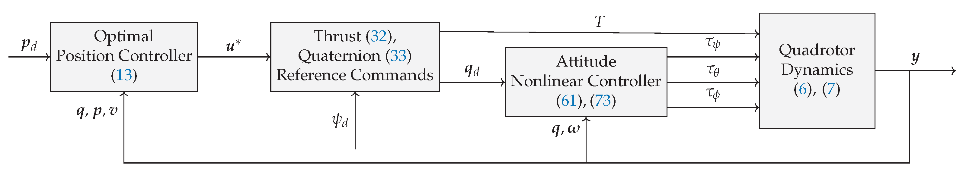
In this section, a nonlinear tracking and control law is derived for the tracking problem stated in Section 2.2. The schematic of the proposed quadrotor controller is presented in Figure 2. By virtue of the underactuated nature of the quadrotor system, a hierarchical strategy is employed to achieve the control development. It consists of an inner loop, the attitude control, combined with an outer loop, the position control, which when bounded provides references to the inner loop. Pontryagin’s principle and the LQR theory aligned with Lyapunov’s theory are at the basis of the controller’s design and the stability proof.
3.1. Position Control
Suppose that the desired position of the quadrotor represented in the inertial frame is . Furthermore, must verify some conditions, namely, it is assumed to be continuous and three-times differentiable. The position error is defined as
with , where is the desired velocity in the body-fixed frame. Define the body velocity error as
In order to achieve zero steady-state error and to add robustness to model uncertainties, a modular integral feedback is taken into account
where and are user-defined.
Hence, by taking the derivative of (8)–(9), considering the position system (6) and the integral dynamics (10), the position tracking system is defined as
where
and is the desired inertial acceleration.
The proposed feedback control law is
where represents the optimal LQR controller for the system (11), , , and are the steady-state LQR gain matrices corresponding to the fully controllable LTI system
Theorem 1.
Consider the dynamics of position error described by (11). The closed-loop system that results from applying the feedback law (13) is globally exponentially stable. Moreover, the feedback law is steady-state optimal in the sense that it minimizes the cost function
where , , and are positive semidefinite matrices, is a positive definite matrix, and .
Proof.
The proof follows a similar approach as in the LQR derivation. Applying the Maximum Principle theorem [31] to minimize the cost function (15) subject to the constraint (11) renders the Hamiltonian H
where is the costate vector of variables, and and are defined in (11). Applying the Maximum Principle theorem [31], the following necessary conditions are obtained:
Hence, the optimal control law is given by
To find a solution for , must be determined. Let , where is a square symmetric matrix, and substitute (17) into the necessary conditions to obtain the equation
which is the Riccati matrix differential equation. Since system (11) is time-varying, will always vary for any t. Consider the following well-defined Lyapunov transformation
Then, as detailed in Appendix A, it is possible to write
which is the Riccati equation for the LTI system (14), and is defined in Appendix A. Consequently, at the infinity, , and the optimal control law (13) can be rewritten as
where . Thereby, is the optimal control law that minimizes the cost function (15) for the position system (11). The proof of global exponential stability is now immediate. Consider the following well-defined Lyapunov function
with the time derivative given by
with and . Thus, and for an x different from zero, and, by [32] [Theorem 4.9], the origin of the closed-loop error system is globally asymptotically stable. To prove exponential stability, observe the following inequalities [32]
where and are the minimum eigenvalue of and the maximum eigenvalue of , respectively, which are positive. Define and apply (25) to (24), which yields
Hence, the origin is globally exponentially stable. □
The block diagram of the position controller is depicted in Figure 3.
The position dynamics are an underactuated system with one control input and three output variables. The outer loop is responsible for generating not only the desired thrust but also angular references. Noting that , although T is a system input, the rotation matrix is not and cannot be set arbitrarily. Nevertheless, the attitude variable can be controlled by means of the attitude system (7), and the input moments can be exploited to drive the thrust force in some intended direction. The input can be rewritten as
where the term is a disturbance due to the attitude error control, is the desired rotation matrix, and describes the discrepancy between the vehicle attitude and the attitude command. The rotation matrix verifies [33]
where denotes the unit quaternion error parameterization that is further defined in Section 3.3, which ensures that through the mapping . The mapping (28) allows to write the perturbation term as
where , and provide an upper bound resorting to the spectral norm of given by
which is a strictly increasing class- function [34]. Keep in mind that similar constraints on can be derived using alternative attitude parameterizations.
The desired quaternion is obtained by equating in (27) with the output of the feedback law (13), which gives
where is the rotation matrix defined in quaternions that represents the chosen yaw angle, i.e., , of the quadrotor, and denotes the desired rotation matrix defined by the equivalent quaternion for a roll rotation followed by a pitch rotation, i.e., . The thrust is computed as
and the desired quaternion command is given by
where
The guidance law (33) only specifies the desired roll and pitch, but it can be extended to include the desired yaw. Let represent the desired yaw quaternion, then the desired quaternion can be defined as follows:
where the operator ⊗ defines the quaternion product, i.e.,
and
Remark 1.
The stability proof presented in this section does not take into consideration the coupling term Δ, which is a requisite when position and attitude are coupled together. In Section 3.2 and Section 3.3, the coupling term Δ is addressed while the attitude controller is deduced and the stability analysis for the overall system is discussed.
The reference angular velocity and its time derivatives along the body’s x and y axes can be readily expressed as functions of , , and their respective time derivatives. In fact, this can be deduced from the kinematic relationship , which implies that
where
and
It is clear that the extracted attitude is time-varying, and that and can be derived using the expressions of and , which are functions of available signals.
3.2. Saturated Control Law
The control law derived in Section 3.1 requires certain conditions to be met. First, due to the nature of the aircraft, the thrust T must be positive, which leads to the following control law requirement
Secondly, the rotors and fans can only manage a maximum thrust, i.e., , which is equivalent to the next requirement
In the context of a well-defined thrust magnitude, the inequalities and can be considered equivalent. Consequently, the last necessary bound for comes from the quaternion extraction (33) and is given by , which is equivalent to the following inequality
In Figure 4, the allowed space for input considering is depicted in light blue and gray. Due to the complexity of finding a smooth saturation function that guarantees these bounds, one could saturate within the gray space; see Figure 4, i.e.,
or even to choose the maximum possible radius sphere around the origin.
To accomplish the requirements in (43), one may employ the following smooth saturation function:
where is the saturation limit, and adjusts the slope transition between linear and saturated regions; see Figure 5.
Given (43) and (44), the saturated control law is designed as follows:
where
with , , , , , where and can be defined by the user such that ,
and , define the allowed saturation limits between each saturation function and satisfy .
Theorem 2.
Let the dynamics of the position error be described by (11). Suppose that the equilibrium of is GAS and LES and that the gain matrices , , and , where , , and . The closed-loop system that results from applying the saturated feedback law (45) achieves global asymptotic stabilization, driving both position and velocity errors to zero for any and chosen such that .
Proof.
The proof can be found in Appendix B. □
Remark 2.
The inclusion of the plant integrator allows the control system to manage constant uncertainties within the dynamic model. For this particular scenario, the Lyapunov function from the preceding theorem can be adapted to account for a constant bias in the position acceleration dynamics. This adaptation can be achieved by employing the methodologies outlined in [20,21] and adjusting them for the application of normed saturation functions. This implies that the proposed system is capable of handling a disturbance provided that .
The preceding theorem guarantees that asymptotically converges to zero. This implies that there exists a time at which tends to , entering the linear region. Consequently, and assuming that also tends asymptotically to zero, the closed-loop system (A4) can be reformulated as
where and .
Lemma 1.
Proof.
The inequalities come to light by setting
and
Then,
□
The graphical illustration in Figure 6 showcases the range of gains concerning the s ratio, from which Theorem 2 and Lemma 1 are satisfied.
Theorem 3.
Let the dynamics of the position error be described by (11) and assume that asymptotically and exhibits exponential local convergence and that the gain matrices , , and , where , , and . Additionally, let (22), which implies that , , and . Choose and , such that in Theorem 1, and let
where , , and . Then, the origin of the closed-loop system that results from applying the saturated feedback law (45) is globally asymptotically stable and locally exponentially stable as soon as . Moreover, the feedback law is steady-state optimal in the sense that it minimizes the cost function
in the linear region.
Proof.
The proof can be found in Appendix C. □
Remark 3.
The saturation law (45), as stipulated in Theorem 3, ensures global asymptotic stability and local exponential stability for the system (11), with the assumption that Δ converges to zero asymptotically and locally exponentially. Moreover, it ensures steady-state optimal control within the linear region of the saturation function and enables the computation of the thrust T and the desired quaternion for every instance.
3.3. Attitude Control—Quaternion
The attitude controller is designed via backstepping to cope with the coupling term . Suppose the desired orientation of the quadrotor is . The quaternion error is a four-dimensional vector, defined as follows:
where represents the inverse of the estimated quaternion rotation, and the error (57) verifies (28).
Define the angular velocity error vector in the body-fixed frame as
where is the desired angular velocity. Take the derivative of (57) and (58), and define the attitude tracking system by the kinematic differential equation
and by the dynamic equation
Apply the following input-to-state linearization control law
and rewrite (59)–(60) as follows:
Define the vectors of variables
and
The objective is to drive and to zero. Note that, due to the dual quaternion representation, two equilibria exist, i.e., . To cope with model imbalances, the control is augmented with an integrator state
Remark 4.
Incorporating plant integrators endows the control system to effectively handle unchanging uncertainties inherent in the dynamical model. As long as these uncertainties are constant, the control system can sustain its properties of stability in both position and attitude error. Nevertheless, when confronted with nonlinear uncertainties, such as those stemming from biased mass or moment of inertia, additional measures are required. The introduction of nonlinear integrative or adaptive terms into the control system emerges as a valuable recourse, effectively reinstating the stability properties and addressing the effects of these nonlinear uncertainties [21].
The quaternion parameter set is redundant due to the fact that a particular attitude of a rigid body will always have two mathematical representations, involving a rotation about an axis relative to each other [35]. Only one of the equilibrium points is considered, i.e., , as formalized with the assumption that follows.
Assumption 1.
The scalar part of the quaternion error maintains its signal for all times, i.e., .
In order to stabilize the equilibrium points of , the signum function, denoted as , is introduced
Remark 5.
In practical scenarios, control continuity is maintained as it hinges on the initial condition . However, it is important to exercise caution if the initial quaternion error is zero and exposed to noise, as this may trigger unwinding behavior. This potential issue can be relaxed through hybrid switching techniques, as detailed in [35,36]. Nonetheless, in a well-defined trajectory, it is typically unrealistic to encounter an initial tracking error that is nearly zero.
A candidate Lyapunov function is devised as
where is defined in (A19), is a positive gain to tune the effects of the coupling term, and is a positive definite diagonal matrix.
Accounting for the coupling term , the Lyapunov function within the saturated region, i.e., , is given by
where . Exploiting the property in (28) and (29), the previous term can be rewritten as follows:
where . The time derivative of is given by
Applying the backstepping procedure, a new error is defined
where is a positive definite gain matrix, and a new Lyapunov function is defined as
with time derivative
The actuation can now be set to cancel the coupling terms and to render the Lyapunov function negative semidefinite. Define the actuation as follows:
where is a positive definite gain matrix.
Theorem 4.
Let the quadrotor kinematics and dynamics be described by (6)–(7), let and be the reference trajectory, and consider the transformation of error coordinates , , , given by (63a), (63b) and (70), respectively. The closed-loop system that results from applying the inputs (45) and (61) achieves trajectory tracking by guaranteeing that the errors , , and converge to zero. Additionally, almost uniform global asymptotic stability of is established.
Proof.
The closed-loop quadrotor error dynamic system, with state variables , , , , and , defined as (63a), (63b), and (70), respectively, with devised according to Theorem 2, admits the Lyapunov function (71) with time derivative
Since , which implies that is compact, and according to [32] [Theorem 4.8], the set is uniformly stable. Resorting to the LaSalle–Yoshizawa Theorem [32] [Theorem 8.4], it follows from (74) that and .
To show uniform asymptotic stability of the equilibrium , one can resort to the Nested Matrosov Theorem [37] [Theorem 1]. Define the following auxiliary function , with time derivative . By inspection, and its time derivative are bounded, and within the set , , yield
Consider the function , with time derivative
Finally, consider the last auxiliary function , which satisfies
By setting for and applying the Nested Matrosov Theorem [37] [Theorem 1], almost uniform global asymptotic stability of is established, since the closed-loop system exhibits a zero measure point for [26].
Therefore, by leveraging the Lyapunov coordinate transformation , it can be asserted that the equilibrium point of the closed-loop system (A4) is also almost globally asymptotically stable. □
The preceding theorem establishes global asymptotic stability for in the context of classical solutions. Nonetheless, it is crucial to exercise caution as this solution is susceptible to arbitrarily small measurement noise near . This vulnerability is underscored in [36], where it is asserted that initial conditions in close proximity to the discontinuity maintain the state near the discontinuity, implying that the condition represents a set of zero measure, rendering the system almost global. This issue can potentially be addressed through hybrid switching techniques, as demonstrated in [38]. However, in practical scenarios where the generated path is well-defined, it is unrealistic for the initial tracking error to be close to 0, and it has been disregarded in this context.
Keep in mind that constructing the Lyapunov function from scratch is possible by utilizing the Lyapunov transformation alongside the position system errors and . This would yield a result akin to applying the transformation at the end of Theorems 2 and 4. However, such an extension of the proof is unnecessary, as the Lyapunov transformation inherently preserves the system’s properties.
Remark 6.
The current approach utilized the principles of backstepping theory to eliminate the interconnection term between position and attitude. Nevertheless, according to Theorem 2, any attitude controller relying exclusively on an attitude parameterization error with asymptotic and locally exponential stability would render the overall system, i.e., position and attitude, asymptotically stable.
4. Implementation
As detailed in Section 3.1, the matrix gains , , and are derived using the LQR method applied to the LTI system (14), and they must adhere to the constraints depicted by the shaded region in Figure 6. An alternative approach involves selecting a specific line, such as , and computing the LQR solution in a manner consistent with Theorem 3.
In order to have some similar sensibility on the gains for the attitude system, the following similar LTI system is considered to compute , , and
By performing the closed-loop system on the attitude system consisting of , , and , and considering only small angle variations, the following system is devised:
where , , and are the LQR gains for the system (78). With some algebraic computations, , , and are retrieved as follows:
where and should be invertible, and , , should check positive definiteness. By considering diagonal input and state matrices while performing the LQR, this is most likely the case, but one must always check. The desired angular velocity and its derivative are computed through (39).
Control Application-Steps
A complete step-by-step approach is outlined below to simplify the applicability of the proposed control law:
- Begin by computing the controller gains, as outlined in the initial part of Section 4;
- Set the maximum thrust and choose p and such that ;
5. Simulation Results
In this section, simulation results are presented to illustrate the performance of the presented control law. The model was simulated in Simulink at a rate of 100 Hz using the equations of motion (6)–(7). The vehicle starts with the states at zero, while the desired position starts at . At 4.5 s, the vehicle takes off, and the position controller is activated at 6 s. Then, the vehicle hovers for around 6 s, and the following lemniscate of Gerono is generated:
and it finishes after two laps.
To ensure smooth transitions, a second-order low-pass filter with a natural frequency of 2 Hz is applied to the trajectory. The vehicle mass is , the inertia matrix is , the thrust is chosen to be bound by , which implies a , the parameter p of the saturation function is set to , and . The transition point from the linear to saturated region is , where . The controller parameters are presented in Table 1, which are used to compute the controller gains, as described in Section 4. The gains for the position controller are selected in accordance with Theorem 3.
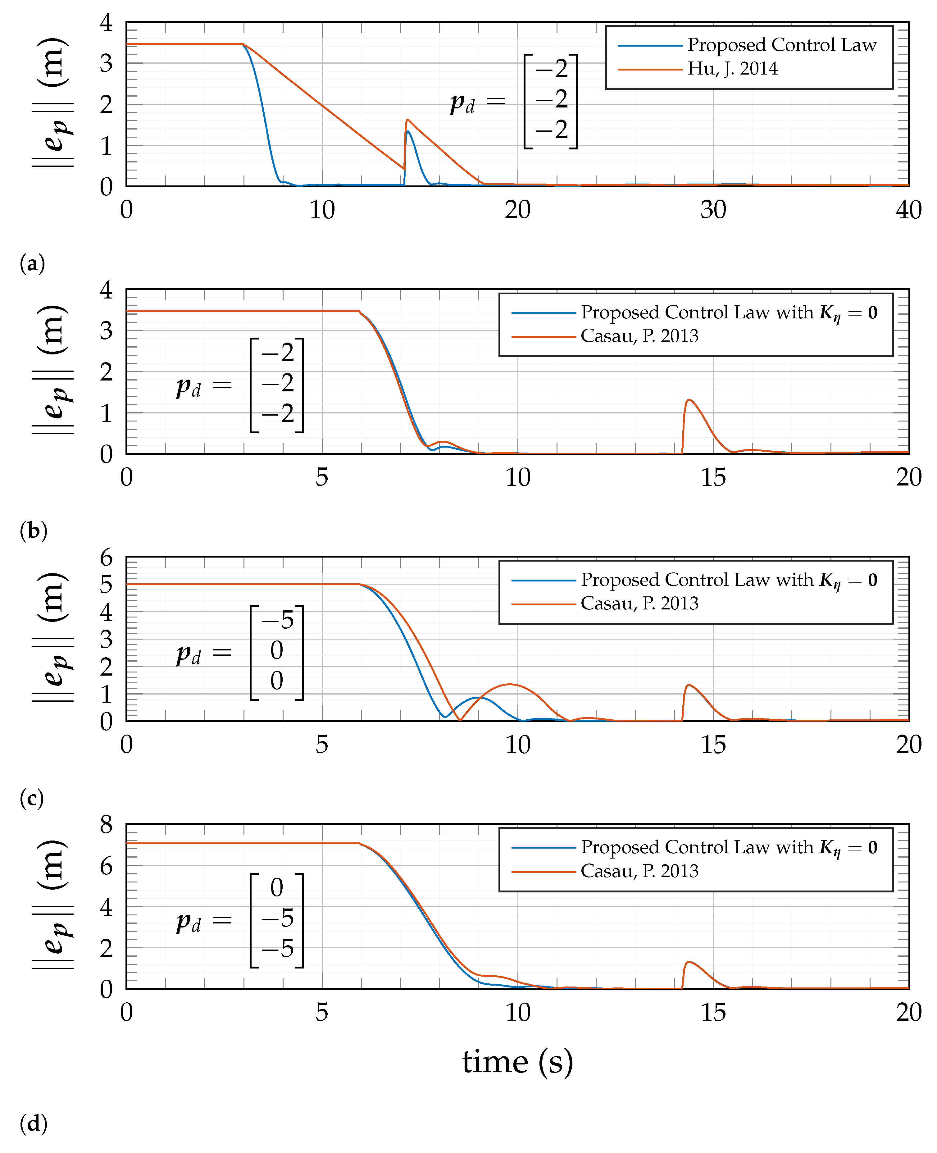
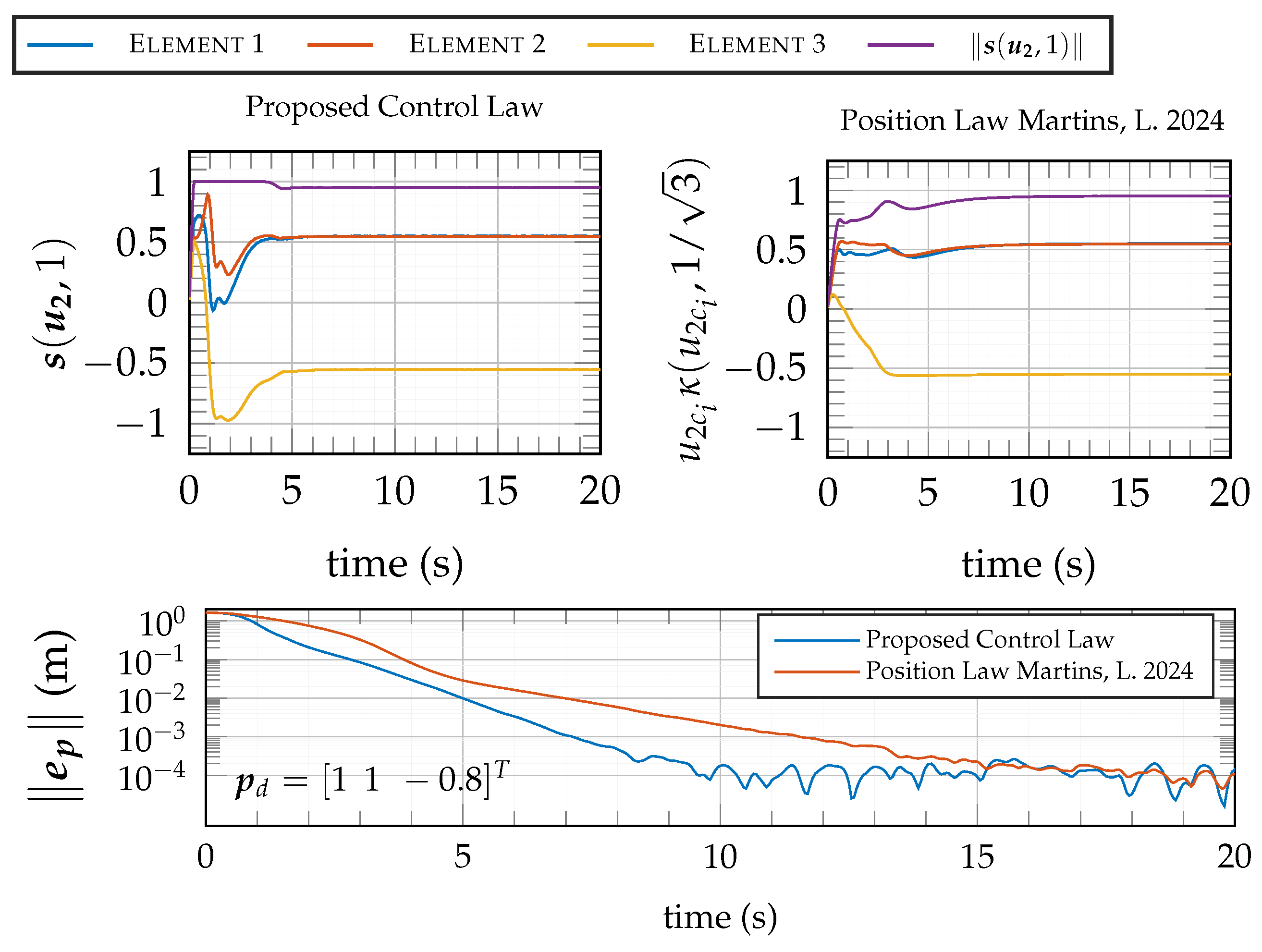
The simulation results are presented in Figure 7, Figure 8 and Figure 9. In Figure 8, the tracking errors converge exponentially to zero, which shows that the proposed solution is capable of following paths. The transient convergence to the pass is less than 3 s. The controller provides zero position and velocity steady-state errors. The rotor, thrust, and moment actuations can be seen in Figure 9, respectively. As illustrated in the bottom left plot of Figure 9, the position controller saturates during the take-off and stays in the imminence of saturation at the time when the trajectory is given. In comparison, the newly proposed position saturation law exhibits a higher convergence rate when contrasted with a conventional nested saturation law [39], as demonstrated in Figure 10. The notable discrepancy in convergence behavior within the saturated region arises from the unique configuration where the position error term is placed on the outer saturation function, as also performed in [12]. This is a departure from the typical nested approach, where the velocity error is positioned on the outer part of the saturation function. Furthermore, the controller is evaluated against the position saturation law described in [40]; see Figure 10. To ensure an equitable assessment, a comparison is made excluding the integrative element of the controller, since the controller proposed in [40] does not have integrative action. The key distinction lies in the saturation approach, where the proposed controller saturates the norm of the input, whereas the controller from [40] applies saturation to each input component individually. The proposed controller exhibits improved convergence rates in the step response, particularly when the step input occurs in one or two directions, as depicted in Figure 10. This enhanced performance can be attributed to the controller’s ability to allocate a larger control action when fewer than three directions are saturated, resulting in faster convergence rates.
Robustness Comparisons
To rigorously evaluate the proposed controller’s effectiveness in counteracting constant biases within the position acceleration dynamics, two distinct scenarios were analyzed. For both scenarios, the system’s maximum tolerable bias threshold was set to , meaning that , with . The system is initialized at a zero position and a step is applied.
In the first scenario, the disturbance is characterized by . Comparative results with the robust position controller from [14] are depicted in Figure 11. This figure illustrates the progression of the integrative saturation action, demonstrating that both controllers successfully converge and neutralize the disturbance. While the position error diminishes to zero for both controllers, the one proposed in this work exhibits superior transient performance. One should notice that the controller in [14] does not account for the bounded normed saturation function, which is the reason why each saturation function is applied individually to each vector element and is bounded by or such that the bound is preserved for all time.
It is important to observe that the controller described in [14] does not incorporate a bounded normed saturation function. Consequently, the saturation function must be applied separately to each element of the vector and bounded by or to ensure that the overall bound is maintained at all times. This requirement may be seen as a drawback, as evidenced in the second scenario that follows.
The second scenario considers a disturbance , with . The outcomes of this test are illustrated in Figure 12. The results demonstrate that the proposed controller successfully manages to cope with the disturbance, driving the position error zero. In contrast, the position controller from [14] fails to achieve this, as its saturation function is unable to handle biases in individual elements exceeding . Essentially, the utilization of a normed bound function allows the system to more effectively distribute the integrative capacity across each variable.
6. Experimental Results
The experimental results attained with the coupled position (32), (45) and attitude controllers (61), on board an AR.Drone 2.0, are presented in Figure 13, Figure 14 and Figure 15. This particular quadrotor offers the capability to implement custom software that can override the factory control system through a Simulink package [41]. This custom software grants direct access to the Pulse Width Modulation (PWM) of each motor. For the experiment, a position tracking system (Qualisys) alongside the onboard IMU of the vehicle was exploited to provide real-time accurate measurements at of position, velocity, quaternion angles, and angular velocity. To allow a fair comparison, the controller parameters and the path generated in the simulation are also used for the real-time experiment.
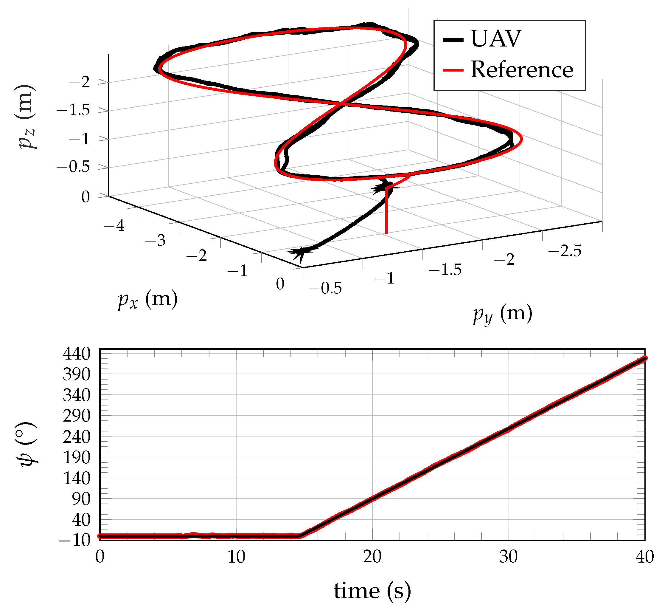
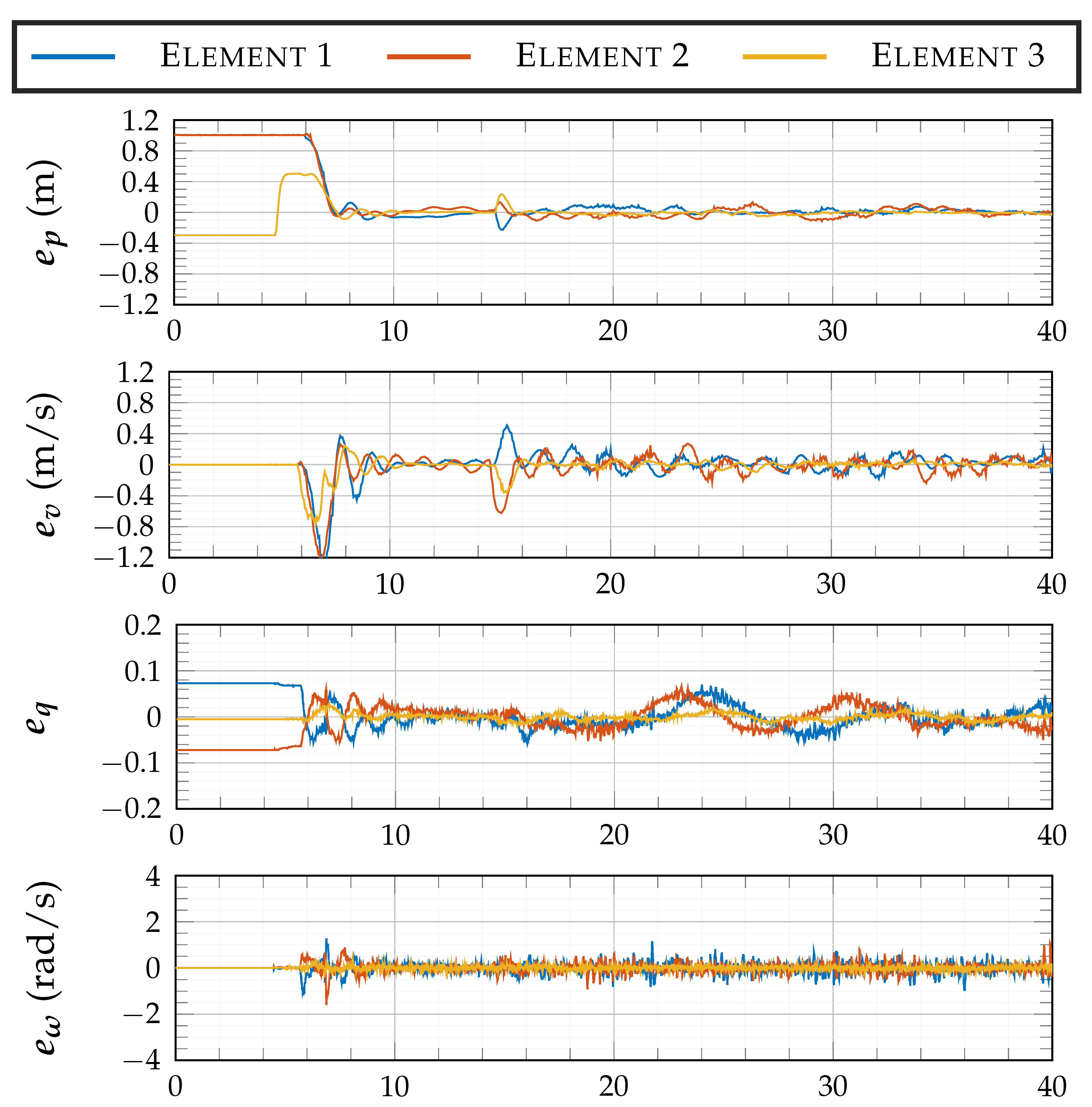
Similarly to the simulation results, the quadrotor starts at 4.5 s from the ground floor and aims to follow a lemniscate path for position and a ramp for the yaw angle. The vehicle starts far off from the initial position in order to trigger saturation of the position control law. In Figure 13, it is shown that the controller was successfully able to track the given path displayed in red. The actual trajectories are displayed in black. The transient convergence to the path occurs within 3 s, and the steady-state error is fewer than 10 cm. The system errors, depicted in Figure 14, converge to the vicinity of zero and remain bounded. The actuations are plotted in Figure 15. The experimental results exhibit an analogous resemblance to the simulation results; see for comparison Figure 7 and Figure 13 and Figure 9 and Figure 15.
Table 2 details the root mean square errors (RMSEs) obtained during the steady state of the trajectory. Furthermore, the entire experiment was recorded, and the result can be seen at https://youtu.be/lg_5mCDDU8s (accessed on 17 April 2024).
7. Conclusions
This paper presented a tracking controller for a quadrotor with steady-state optimal properties, developed on the body-fixed frame and quaternion space. The controller stabilizes the position and attitude of a rigid body robustly and almost globally asymptotically. Through a specific set of transformation matrices, the positioning system is rendered LTI, allowing the exploitation of linear control techniques that optimally stabilize it. To avoid the physical limitations of the vehicle, during the thrust and attitude references extraction, a saturation law with modular integrative action that bounds the norm of the position input is devised, ensuring GAS and LES for the position system when paired with any controller that achieves LES for the attitude system. At first, the position and attitude are addressed separately. The origin of the saturation position controller exhibits global asymptotic stability in the saturated region and exponential stability in the linear region. The attitude controller, derived from the backstepping technique, tackles the effect of the interconnection term , which results in almost uniform global asymptotic stability of the overall closed-loop system. Experimental and simulation results were shown to assess the performance of the proposed controller.
Author Contributions
J.M., methodology, software, validation, and writing—original draft; C.C., P.O., P.B. and C.S., supervision, writing—review and editing, project administration, and funding acquisition. All authors have read and agreed to the published version of the manuscript.
Funding
This work was supported by the Portuguese Fundação para a Ciência e a Tecnologia (FCT) through the scholarship 2020.06736.BD, and the Institute for Mechanical Engineering (IDMEC), under the projects LAETA Base Funding (DOI: 10.54499/UIDB/50022/2020) and LAETA Programatic Funding (DOI: 10.54499/UIDP/50022/2020), through Institute for Systems and Robotics (ISR), under LARSyS funding (DOI: 10.54499/LA/P/0083/2020, 10.54499/UIDP/50009/2020, and 10.54499/UIDB/50009/2020) and by the University of Macau, Macau, China, under Projects MYRG 2022-00205-FST and MYRG-GRG2023-00107-FST-UMDF. This work has also been supported by the European Union under the Next Generation EU, through a grant of the Portuguese Republic’s Recovery and Resilience Plan (PRR) Partnership Agreement, within the scope of the project PRODUTECH R3—“Agenda Mobilizadora da Fileira das Tecnologias de Produção para a Reindustrialização”, Total project investment: 166.988.013,71 Euros; Total Grant: 97.111.730,27 Euros.
Data Availability Statement
The data used in the present work are all available in the document itself.
Conflicts of Interest
The authors declare no conflicts of interest.
Appendix A
Appendix B
Proof of Theorem 2.
Let position and velocity error dynamics subjected to the input saturation be given by
and consider for now there is no inner-loop tracking error, i.e., . By applying the Lyapunov transformation of coordinates
to the closed-loop system (A4) results in the following LTI system with saturation input
where
and . From here onwards, the second term in the saturation function will be omitted. Hence, if achieves asymptotic stabilization for the system (A6), the stability characteristics are then extended, through the Lyapunov transformation, to the system (11) with saturated feedback law (45).
Inspired by [40], the following radially unbounded Lyapunov function is devised:
where , , , , , and is a positive definite symmetric matrix. The time derivative is given by
By choosing , and
the following expression is obtained:
Since (47) is positive definite, choosing , and any such that , it is possible to verify that is negative semidefinite. Since (A8) is radially unbounded, then for any initial condition (, , )(0), the sublevel set
is compact. It follows from [32] [Theorem 4.8] that the set is globally stable, and it follows from [32] [Theorem 8.4] that converges to 0; therefore, each solution converges to 0 asymptotically. Then, the origin of the closed-loop system (A6) is globally asymptotically stable.
Accounting for the interconnection term , the system (A6) can be written as
where , and represents any parameterization of the attitude error. Notice that is bounded by a class- function (30) and does not depend on , and that can be bounded by
for some and . Then, by following the proof in [34] [Theorem 4.7], the fact that the system (A12) is forward complete [42] and due to the assumption that the equilibrium of is to be GAS and LES, it can be deduced that there exists a time for which exponentially converges to zero. Consequently, there exists a constant and a function , such that
for . This analysis establishes the boundedness of . Given that is radially unbounded, the boundedness of implies the boundedness of . Hence, the GAS of the equilibrium point follows. Therefore, by leveraging the Lyapunov coordinate transformation (A5), it can be asserted that the equilibrium point of the closed-loop system (A4) is globally asymptotically stable. □
Appendix C
Proof of Theorem 3.
By choosing and , then , which satisfies the initial inequality in Theorem 1. As a result, tends to zero asymptotically, and there exists a time at which the original system (A4) converges to the system (49).
Following the same logic as in the beginning of Theorem 2, if one applies the transformation of coordinates
to the closed-loop system (49) results in the following LTI system with saturation input
where , , and represent the LQR gains that minimize the cost function (56). These gains correspond to the matrices derived from the positive definite solution of the following Riccati equation
where the solutions for , , and are given by
which is a subtly distinct solution compared with the conventional LQR solution, as in this instance the state matrix in (A16) is dependent on matrix . Hence, if achieves asymptotic stabilization for the system (A16), the stability characteristics are then extended, through the Lyapunov transformation , to the closed-loop system (49).
A candidate unbounded Lyapunov function for system (A16) is
where . The time derivative of (A19) is given by
where with as in (47). According to Theorem 2 and Lemma 1, enters the linear region in finite time. Meaning that after a , and . Consequently, can be written as
which is negative semidefinite for any , where , and a and c are given in (53)–(52), respectively, for and . The Lyapunov function (A19) admits for the following upper bound:
Since , one can show that for some . Consequently, one can write
It follows that the origin of the closed-loop system (A16) is globally exponentially stable. Therefore, leveraging the Lyapunov coordinate transformation , it can be asserted that for , , and , , and given by (55), the equilibrium point of the closed-loop system (49) is globally exponentially stable, as there is time such that , meaning that the closed-loop system will converge to
which falls under the systems outlined by Theorem 1. □
References
- Pounds, P.; Mahony, R.; Corke, P. Modelling and control of a large quadrotor robot. Control Eng. Pract. 2010, 18, 691–699. [Google Scholar] [CrossRef]
- Liang, H.; Lee, S.C.; Bae, W.; Kim, J.; Seo, S. Towards UAVs in Construction: Advancements, Challenges, and Future Directions for Monitoring and Inspection. Drones 2023, 7, 202. [Google Scholar] [CrossRef]
- Hua, M.D.; Hamel, T.; Morin, P.; Samson, C. Introduction to feedback control of underactuated VTOLvehicles: A review of basic control design ideas and principles. IEEE Control Syst. Mag. 2013, 33, 61–75. [Google Scholar] [CrossRef]
- Emran, B.J.; Najjaran, H. A review of quadrotor: An underactuated mechanical system. Annu. Rev. Control 2018, 46, 165–180. [Google Scholar] [CrossRef]
- Sonugür, G. A Review of quadrotor UAV: Control and SLAM methodologies ranging from conventional to innovative approaches. Robot. Auton. Syst. 2023, 161, 104342. [Google Scholar] [CrossRef]
- Wan, M.; Chen, M.; Lungu, M. Integral Backstepping Sliding Mode Control for Unmanned Autonomous Helicopters Based on Neural Networks. Drones 2023, 7, 154. [Google Scholar] [CrossRef]
- Martins, L.; Cardeira, C.; Oliveira, P. Linear Quadratic Regulator for Trajectory Tracking of a Quadrotor. IFAC-PapersOnLine 2019, 52, 176–181. [Google Scholar] [CrossRef]
- Martins, L.; Cardeira, C.; Oliveira, P. Feedback Linearization with Zero Dynamics Stabilization for Quadrotor Control. J. Intell. Robot. Syst. 2021, 101, 1–17. [Google Scholar] [CrossRef]
- Ha, C.; Zuo, Z.; Choi, F.B.; Lee, D. Passivity-based adaptive backstepping control of quadrotor-type UAVs. Robot. Auton. Syst. 2014, 62, 1305–1315. [Google Scholar] [CrossRef]
- Mellinger, D.; Kumar, V. Minimum snap trajectory generation and control for quadrotors. In Proceedings of the 2011 IEEE International Conference on Robotics and Automation, Shanghai, China, 9–13 May 2011; pp. 2520–2525. [Google Scholar]
- Invernizzi, D.; Lovera, M. Trajectory tracking control of thrust-vectoring UAVs. Automatica 2018, 95, 180–186. [Google Scholar] [CrossRef]
- Invernizzi, D.; Lovera, M.; Zaccarian, L. Integral ISS-Based Cascade Stabilization for Vectored-Thrust UAVs. IEEE Control Syst. Lett. 2020, 4, 43–48. [Google Scholar] [CrossRef]
- Gamagedara, K.; Bisheban, M.; Kaufman, E.; Lee, T. Geometric Controls of a Quadrotor UAV with Decoupled Yaw Control. In Proceedings of the 2019 American Control Conference (ACC), Philadelphia, PA, USA, 10–12 July 2019; pp. 3285–3290. [Google Scholar] [CrossRef]
- Martins, L.; Cardeira, C.; Oliveira, P. Global trajectory tracking for quadrotors: An MRP-based hybrid strategy with input saturation. Automatica 2024, 162, 111521. [Google Scholar] [CrossRef]
- Control of VTOL Vehicles with Thrust-Tilting Augmentation. IFAC Proc. Vol. 2014, 47, 2237–2244. [CrossRef]
- Naldi, R.; Furci, M.; Sanfelice, R.G.; Marconi, L. Robust Global Trajectory Tracking for Underactuated VTOL Aerial Vehicles Using Inner-Outer Loop Control Paradigms. IEEE Trans. Autom. Control 2017, 62, 97–112. [Google Scholar] [CrossRef]
- Quadrotor trajectory generation and tracking for aggressive maneuvers with attitude constraints. IFAC-Pap. 2019, 52, 55–60.
- Cabecinhas, D.; Cunha, R.; Silvestre, C. A Globally Stabilizing Path Following Controller for Rotorcraft with Wind Disturbance Rejection. IEEE Trans. Control Syst. Technol. 2015, 23, 708–714. [Google Scholar] [CrossRef]
- Cabecinhas, D.; Cunha, R.; Silvestre, C. A nonlinear quadrotor trajectory tracking controller with disturbance rejection. Control Eng. Pract. 2014, 26, 1–10. [Google Scholar] [CrossRef]
- Casau, P.; Sanfelice, R.G.; Cunha, R.; Cabecinhas, D.; Silvestre, C. Robust global trajectory tracking for a class of underactuated vehicles. Automatica 2015, 58, 90–98. [Google Scholar] [CrossRef]
- Xie, W.; Cabecinhas, D.; Cunha, R.; Silvestre, C. Adaptive Backstepping Control of a Quadcopter with Uncertain Vehicle Mass, Moment of Inertia, and Disturbances. IEEE Trans. Ind. Electron. 2021, 69, 549–559. [Google Scholar] [CrossRef]
- Nicotra, M.M.; Garone, E. Explicit reference governor for continuous time nonlinear systems subject to convex constraints. In Proceedings of the 2015 American Control Conference (ACC), Chicago, IL, USA, 1–3 July 2015; pp. 4561–4566. [Google Scholar] [CrossRef]
- Osorio, J. Reference Governors: From Theory to Practice. Ph.D. Thesis, Electrical Engineering Department, University of Vermont, Burlington, VT, USA, 2020. [Google Scholar]
- Nicotra, M.; Naldi, R.; Garone, E. A robust explicit reference governor for constrained control of Unmanned Aerial Vehicles. In Proceedings of the 2016 American Control Conference (ACC), Boston, MA, USA, 6–8 July 2016; pp. 6284–6289. [Google Scholar] [CrossRef]
- Convens, B.; Merckaert, K.; Nicotra, M.; Naldi, R.; Garone, E. Control of Fully Actuated Unmanned Aerial Vehicles with Actuator Saturation. In Proceedings of the IFAC 2017 World Congress, Toulouse, France, 9–14 July 2017. [Google Scholar] [CrossRef]
- Bhat, S.; Bernstein, D. A topological obstruction to global asymptotic stabilization of rotational motion and the unwinding phenomenon. In Proceedings of the 1998 American Control Conference. ACC (IEEE Cat. No.98CH36207), Philadelphia, PA, USA, 26 June 1998; Volume 5, pp. 2785–2789. [Google Scholar]
- Optimal position and velocity navigation filters for autonomous vehicles. Automatica 2010, 46, 767–774. [CrossRef]
- Cao, N.; Lynch, A.F. Inner–Outer Loop Control for Quadrotor UAVs With Input and State Constraints. IEEE Trans. Control Syst. Technol. 2016, 24, 1797–1804. [Google Scholar] [CrossRef]
- Allibert, G.; Abeywardena, D.; Bangura, M.; Mahony, R. Estimating Body-Fixed Frame Velocity and Attitude from Inertial Measurements for a Quadrotor Vehicle. In Proceedings of the 2014 IEEE Conference on Control Applications, CCA 2014, Antibes/Nice, France, 8–10 October 2014. [Google Scholar]
- Lefeber, E.; van den Eijnden, S.; Nijmeijer, H. Almost global tracking control of a quadrotor UAV on SE(3). In Proceedings of the 2017 IEEE 56th Annual Conference on Decision and Control (CDC), Melbourne, VIC, Australia, 12–15 December 2017; pp. 1175–1180. [Google Scholar] [CrossRef]
- Front Matter. In Optimal Control; John Wiley & Sons, Ltd.: Hoboken, NJ, USA, 2012; pp. i–xii. [CrossRef]
- Khalil, H.K. Nonlinear Systems, 3rd ed.; Prentice-Hall: Upper Saddle River, NJ, USA, 2002. [Google Scholar]
- Bani Younes, A.; Mortari, D. Derivation of All Attitude Error Governing Equations for Attitude Filtering and Control. Sensors 2019, 19, 4682. [Google Scholar] [CrossRef] [PubMed]
- Sepulchre, R.; Jankovic, M.; Kokotovic, P. Constructive Nonlinear Control; Communications and Control Engineering; Springer: London, UK, 1997. [Google Scholar]
- Schlanbusch, R.; Loria, A.; Nicklasson, P.J. On the stability and stabilization of quaternion equilibria of rigid bodies. Automatica 2012, 48, 3135–3141. [Google Scholar] [CrossRef]
- Mayhew, C.G.; Sanfelice, R.G.; Teel, A.R. Quaternion-Based Hybrid Control for Robust Global Attitude Tracking. IEEE Trans. Autom. Control 2011, 56, 2555–2566. [Google Scholar] [CrossRef]
- Loria, A.; Panteley, E.; Popovic, D.; Teel, A. A nested Matrosov theorem and persistency of excitation for uniform convergence in stable nonautonomous systems. IEEE Trans. Autom. Control 2005, 50, 183–198. [Google Scholar] [CrossRef]
- Mayhew, C.G.; Sanfelice, R.G.; Teel, A.R. Robust global asymptotic attitude stabilization of a rigid body by quaternion-based hybrid feedback. In Proceedings of the 48h IEEE Conference on Decision and Control (CDC) Held Jointly with 2009 28th Chinese Control Conference, Shanghai, China, 15–18 December 2009; pp. 2522–2527. [Google Scholar] [CrossRef]
- Hu, J.; Zhang, H. Globally asymptotically stable saturated PID controllers for a double integrator with constant disturbance. Int. J. Robust Nonlinear Control 2014, 24. [Google Scholar] [CrossRef]
- Casau, P.; Sanfelice, R.G.; Cunha, R.; Cabecinhas, D.; Silvestre, C. Global trajectory tracking for a class of underactuated vehicles. In Proceedings of the 2013 American Control Conference, Washington, DC, USA, 17–19 June 2013; pp. 419–424. [Google Scholar] [CrossRef]
- Lee, D.A.R. Drone 2.0 Support from Embedded Coder. 2016. Available online: https://www.mathworks.com/hardware-support/ar-drone.html (accessed on 17 April 2024).
- Mironchenko, A. Input-to-State Stability: Theory and Applications; Springer: Cham, Switzerland, 2023. [Google Scholar]
Figure 1.
Quadrotor model.

Figure 2.
Controller architecture.

Figure 3.
Position controller block diagram.

Figure 4.
Two-dimensional bounds for the input , considering , according to (43) in gray. The total admissible area also aggregates the light blue area, which results from (40) (red circle), (41) (blue circle), and (42) (green lines).

Figure 5.
Saturation function (44) and the respective derivative for .
Figure 5.
Saturation function (44) and the respective derivative for .

Figure 6.
Graphical representation of the inequalities from Lemma 1. The shaded region indicates the allowable region for the modular integral feedback concerning the ratio .
Figure 6.
Graphical representation of the inequalities from Lemma 1. The shaded region indicates the allowable region for the modular integral feedback concerning the ratio .

Figure 7.
Simulated tridimensional response obtained with the quadrotor during trajectory tracking with the proposed nonlinear control approach, from top to bottom: tridimensional; yaw angle.
Figure 7.
Simulated tridimensional response obtained with the quadrotor during trajectory tracking with the proposed nonlinear control approach, from top to bottom: tridimensional; yaw angle.

Figure 8.
Error state variables during the simulation.

Figure 9.
Thrust, moments, and norm of the position saturation control law resulting from the control law implemented during the simulation.
Figure 9.
Thrust, moments, and norm of the position saturation control law resulting from the control law implemented during the simulation.

Figure 10.
Transient performance comparison of the proposed position saturation law with, from top to bottom, (a) a nested solution as per [39] and (b–d) the controller detailed in [40] under various initial conditions. (a) Comparison with the nested solution in [39] with . (b) Comparison with the position controller in [40] with . (c) Comparison with the position controller in [40] with . (d) Comparison with the position controller in [40] with .

Figure 11.
Comparison of the proposed position controller with the position controller presented in [14]. The upper plot demonstrates the integration action compensating for a constant system bias , with the lower plot illustrating the norm of the position error.
Figure 11.
Comparison of the proposed position controller with the position controller presented in [14]. The upper plot demonstrates the integration action compensating for a constant system bias , with the lower plot illustrating the norm of the position error.

Figure 12.
Comparison of the proposed controller with the controller presented in [14]. The upper plot demonstrates the integration action compensating for a constant system bias , with the lower plot illustrating the norm of the position error.
Figure 12.
Comparison of the proposed controller with the controller presented in [14]. The upper plot demonstrates the integration action compensating for a constant system bias , with the lower plot illustrating the norm of the position error.

Figure 13.
Tridimensional response (upper) and yaw angle response (lower) obtained with the quadrotor during trajectory tracking.
Figure 13.
Tridimensional response (upper) and yaw angle response (lower) obtained with the quadrotor during trajectory tracking.

Figure 14.
Error state variables during the experiment.

Figure 15.
Thrust, moments, and norm of the position saturation control law resulting from the control law implemented during the experimental validation.
Figure 15.
Thrust, moments, and norm of the position saturation control law resulting from the control law implemented during the experimental validation.


Table 1.
Controller parameters: Input and state matrices to compute the controller gains, as described in Section 4 and Theorem 3.
Table 1.
Controller parameters: Input and state matrices to compute the controller gains, as described in Section 4 and Theorem 3.
| (55) | (55) | (55) | |||||
|---|---|---|---|---|---|---|---|
| 93 | 20 | 0.1 | 0.02 |
Table 2.
Root mean square error obtained in the experimental test.
| 0.0373 | 0.0580 | 0.0189 |
Disclaimer/Publisher’s Note: The statements, opinions and data contained in all publications are solely those of the individual author(s) and contributor(s) and not of MDPI and/or the editor(s). MDPI and/or the editor(s) disclaim responsibility for any injury to people or property resulting from any ideas, methods, instructions or products referred to in the content. |
© 2024 by the authors. Licensee MDPI, Basel, Switzerland. This article is an open access article distributed under the terms and conditions of the Creative Commons Attribution (CC BY) license (https://creativecommons.org/licenses/by/4.0/).
Share and Cite
MDPI and ACS Style
Madeiras, J.; Cardeira, C.; Oliveira, P.; Batista, P.; Silvestre, C. Saturated Trajectory Tracking Controller in the Body-Frame for Quadrotors. Drones 2024, 8, 163. https://doi.org/10.3390/drones8040163
AMA Style
Madeiras J, Cardeira C, Oliveira P, Batista P, Silvestre C. Saturated Trajectory Tracking Controller in the Body-Frame for Quadrotors. Drones. 2024; 8(4):163. https://doi.org/10.3390/drones8040163
Chicago/Turabian StyleMadeiras, João, Carlos Cardeira, Paulo Oliveira, Pedro Batista, and Carlos Silvestre. 2024. "Saturated Trajectory Tracking Controller in the Body-Frame for Quadrotors" Drones 8, no. 4: 163. https://doi.org/10.3390/drones8040163