1. Introduction
Over the past thirty years, with the long-term development of Global Navigation Satellite System (GNSS) basic services, the basic needs of the UAV field for Positioning, Navigation, and Timing (PNT) have been met, making it the mainstream option for UAV navigation and positioning [
1]. However, the disadvantages of GNSS positioning technology have become increasingly apparent. GNSS signals have low power and are susceptible to interference. They are severely limited in scenarios where signals are blocked or in urban multipath jamming environments, to the extent that they cannot provide effective positioning services for UAVs [
2,
3,
4]. These factors have become important constraints affecting further development in the UAV field [
5,
6]. To address these limitations, using SOP technology has proven effective for positioning [
7]. This technology leverages any available non-navigation/non-cooperative signals, extracting relevant observations to achieve terminal localization. Its advantages lie in its ability to use existing infrastructure without the need for additional construction. SOP technology boasts wide signal spectrum coverage, high ground power levels, and robust anti-jamming capabilities. As a result, SOP positioning has become a research hotspot as a promising solution to overcoming the limitations of UAVs using GNSS positioning technology [
8].
SOPs are primarily categorized into terrestrial [
9,
10,
11,
12] and celestial opportunity signals [
13]. Compared to terrestrial signals, celestial signals offer advantages such as extensive coverage and a wide frequency range, enabling seamless global positioning in complex geographical environments. Simultaneously, the rapid development of emerging LEO satellite communication constellations, represented by Starlink and OneWeb, has been notable. The global number of satellites in LEO for communication purposes is anticipated to surpass 22,000 by 2025 [
14]. This vast quantity of LEO satellites will provide abundant radiation sources for celestial SOP positioning. In this context, the use of LEO constellations for SOP positioning has become a research hotspot. Numerous studies [
15,
16,
17,
18,
19,
20,
21,
22] have introduced cases where research teams leverage LEO satellites for positioning. Recent research findings indicate that a positioning accuracy of <15 m can be achieved [
23].
The accuracy of LEO satellite SOP positioning technology has steadily approached the level of GNSS positioning. This advancement has allowed it to meet the precision requirements for UAV positioning in daily scenarios. The goal is to provide independent, reliable, and high-precision positioning services for UAVs, leveraging the numerous advantages offered by LEO satellite SOP positioning. Simultaneously, with the development of miniaturization technology for SOP positioning terminals, this technology’s application to the UAV positioning field has become crucial for the development of UAVs. The goal of this trend is to achieve independent and high-precision positioning services for UAVs with the benefits presented by LEO satellite SOP positioning technology.
However, the scenario of drone operation is often accompanied by various adverse electromagnetic environments, such as urban multipath jamming and malicious human jamming, as shown in
Figure 1. Therefore, researching anti-jamming algorithms focused on LEO satellite SOP positioning has extremely high application value for drones.
At present, there is no research on anti-jamming technologies specifically tailored to LEO satellite SOP positioning, either domestically or internationally. Previous achievements in anti-jamming technology mainly focused on GNSS positioning. According to the types of receiving terminal antennas, they can be divided into single-antenna and antenna array anti-jamming technology. The principle of single-antenna anti-jamming technology is to suppress interference spectral lines. According to the processing domain, approaches can be divided into time domain and frequency domain anti-jamming algorithms. The antenna array anti-jamming technology uses multiple antenna elements. According to the different incident directions of the signal and jamming, interference cancellation is performed using vector weighting, mainly using spatial domain anti-jamming algorithms [
24,
25,
26,
27,
28,
29,
30,
31,
32,
33]. Compared with antenna arrays, single antennas are widely used in the drone field due to their small size, low cost, and low power consumption.
The single-antenna time–frequency domain anti-jamming algorithm is based on the premise that the navigation signal is much weaker than the noise. It assumes that the power spectrum of the superimposed signal and noise is flat and that the spectral lines at different frequencies follow the same distribution. It then calculates the interference detection threshold for anti-jamming processing. In a scenario with strong signals, however, the statistical characteristics of the spectral lines at different frequencies are correlated with the frequency due to the presence of strong signals. This requires different interference detection thresholds for the same false alarm probability, leading to a higher false alarm probability or lower detection probability, rendering the anti-jamming algorithm ineffective [
34,
35].
Conventional anti-jamming methods cannot be directly applied due to the distinct characteristics of LEO satellite signals, such as a high ground SNR (typically ranging from 15–30 dB) and narrow downlink bandwidths, which significantly differ from traditional satellite navigation signals. This issue is particularly challenging in the context of time–frequency domain anti-jamming scenarios, widely used in UAV applications with single-antenna receivers. For scenarios with high SNRs and strong signals, most traditional research has focused on spatial domain anti-jamming algorithms using antenna array techniques [
34,
35,
36,
37,
38,
39,
40]. However, there is limited research on time–frequency domain anti-jamming algorithms applicable to single-antenna receivers due to the presence of strong signals, which significantly affect jamming threshold settings and lead to high false alarm rates or low detection probabilities. Currently, only two studies in the literature mention frequency domain anti-jamming algorithms suitable for strong signal scenarios [
34,
35]. One of them, the Anti-Jamming Weighting Generation (AJWG) algorithm [
34], optimizes the equivalent carrier-to-noise ratio (CNR) at the despread output for each spectral line of the signal, deciding whether the signal’s single spectral line is jamming before subsequently eliminating or preserving it. Due to the excessively large computational complexity of the AJWG algorithm, it is rarely used in engineering applications. Therefore, this paper does not further analyze the AJWG algorithm.
This study conducted research on single-antenna anti-jamming technology for LEO satellite SOP positioning. Firstly, the other GNSS frequency domain anti-jamming improvement algorithm was analyzed, revealing several flaws when directly applied to the anti-jamming scenario in UAVs using LEO satellite SOP positioning. Secondly, considering the narrow downlink bandwidth and high ground SNR characteristics of LEO satellite constellation signals, a Consecutive Iteration based on Signal Cancellation (SCCI) algorithm was proposed, which significantly reduces the errors generated during the model fitting process. Additionally, an adaptive variable convergence factor was designed to address the challenge of balancing convergence speed and steady-state error during iterations. Finally, to verify the jamming suppression performance of the proposed algorithm, simulations and experimental validations were conducted in different scenarios. The results show that compared to traditional algorithms, the proposed algorithm significantly improves the frequency domain anti-jamming performance in LEO satellite SOP positioning anti-jamming scenarios for UAVs.
2. The Consecutive Mean Excision Based on Signal Cancellation (SCCME) Algorithm [35]
The other GNSS frequency domain anti-jamming improvement algorithm is the SCCME algorithm. The concept behind the SCCME algorithm involves iteratively approximating and fitting the power spectrum of strong signals. This process aims to eliminate the impact of strong signal power on the input signal, thereby transforming the anti-jamming issue in strong-signal scenarios into a conventional interference detection problem in weak-signal scenarios. The authors considered that the power spectrum of the input signal (signal and noise) in strong-signal scenarios follows a chi-square distribution. Consequently, they derived a first-order expression relating the power spectrum of the input signal to the power spectral density of the signal. Subsequently, they constructed an approximation model:
where
represents the estimated power spectrum of the input signal,
denotes the power spectrum of the signal, and a and b are parameter variables.
Assuming that the input signal power spectrum is denoted as , the authors employed the gradient descent method. They minimized the mean square error between and the model estimate . The estimated values of parameters a and b in Equation (1) were obtained through iterations. Consequently, they derived an estimate of the mean of the input signal power spectrum . In the subsequent step, the estimated power spectrum mean obtained from the model was subtracted from the input signal power spectrum . This operation was interpreted as removing the power spectrum values corresponding to signal components in the input signal, retaining only the noise and jamming signal components.
According to the flow of this algorithm, it is evident that during the iterative estimation of , the algorithm tends to overestimate the signal power spectral density due to the criterion of minimizing the mean square error between and and considering that jamming power is often much greater than signal or noise power in practical scenarios. The process of canceling out the estimated from may lead to the removal of some noise power, making it challenging to statistically characterize the remaining noise power distribution. However, in frequency domain anti-jamming, the premise for setting detection thresholds involves the statistical characteristics of the amplitude spectrum. In other words, the statistical characteristics of spectral lines at different frequencies should be consistent. In this case, due to the over-removal of noise power, spectral lines’ statistical characteristics at different frequencies become inconsistent and are correlated with the frequency. Setting the interference detection thresholds according to the original statistical characteristics results in an inflated false alarm probability or a reduced detection probability. Inflated false alarm probabilities may cause more interference-free spectral lines to be misjudged as jamming signals and zeroed out, introducing greater anti-jamming losses. Conversely, a reduced detection probability may result in residual interference spectral lines, affecting the anti-jamming performance.
Such interference detection errors may be tolerable when confronting satellite navigation signals with downlink bandwidths, commonly in the tens of megahertz. However, due to the generally narrow downlink signal bandwidth of LEO satellites (e.g., Iridium system with a bandwidth of 500 kHz and Orbcomm system with only 25 kHz), errors in interference detection can significantly impact the signal quality after anti-jamming processing.
3. The Consecutive Iteration Based on Signal Cancellation (SCCI) Algorithm
In this section, building upon the principles of the SCCME algorithm and utilizing the Least Mean Square (LMS) principle, we propose an algorithm known as SCCI. This algorithm has an optimized workflow and incorporates an adaptive variable convergence factor in its process for the characteristics of LEO satellite downlink signals. The final simulation compares the convergence factors of the SCCI algorithm and the SCCME algorithm, validating that the adaptive convergence factor of the SCCI algorithm can better balance between a faster convergence speed and smaller steady-state error during the iteration process.
3.1. Process Optimization
The core objective of optimizing the SCCI algorithm workflow was to reduce the impact of jamming power on the model estimate . This reduction minimizes the difference between the final estimated value of and the true signal power spectrum . This optimization accurately sets the false alarm probability for the next step. Therefore, the steps after obtaining the estimated value in the improved algorithm are essentially consistent with the SCCME algorithm. The main difference lies in how the estimated value is obtained. The following explanation will focus on this aspect.
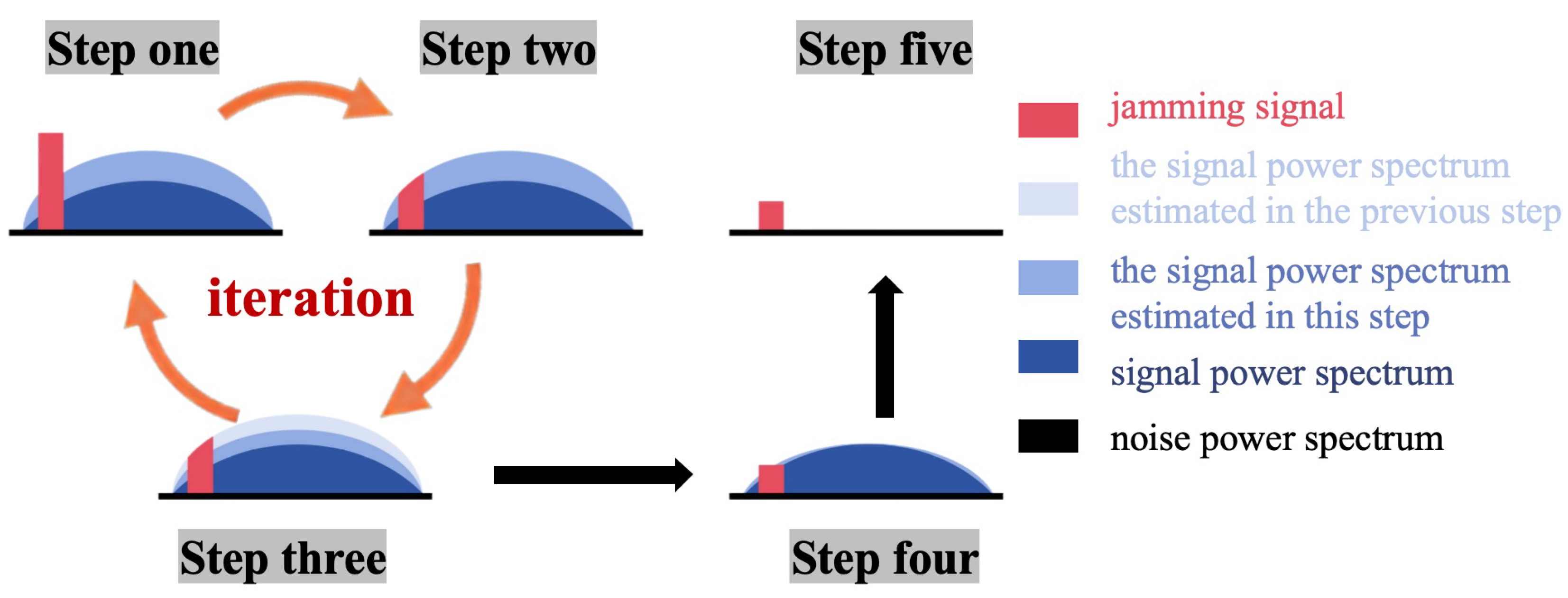
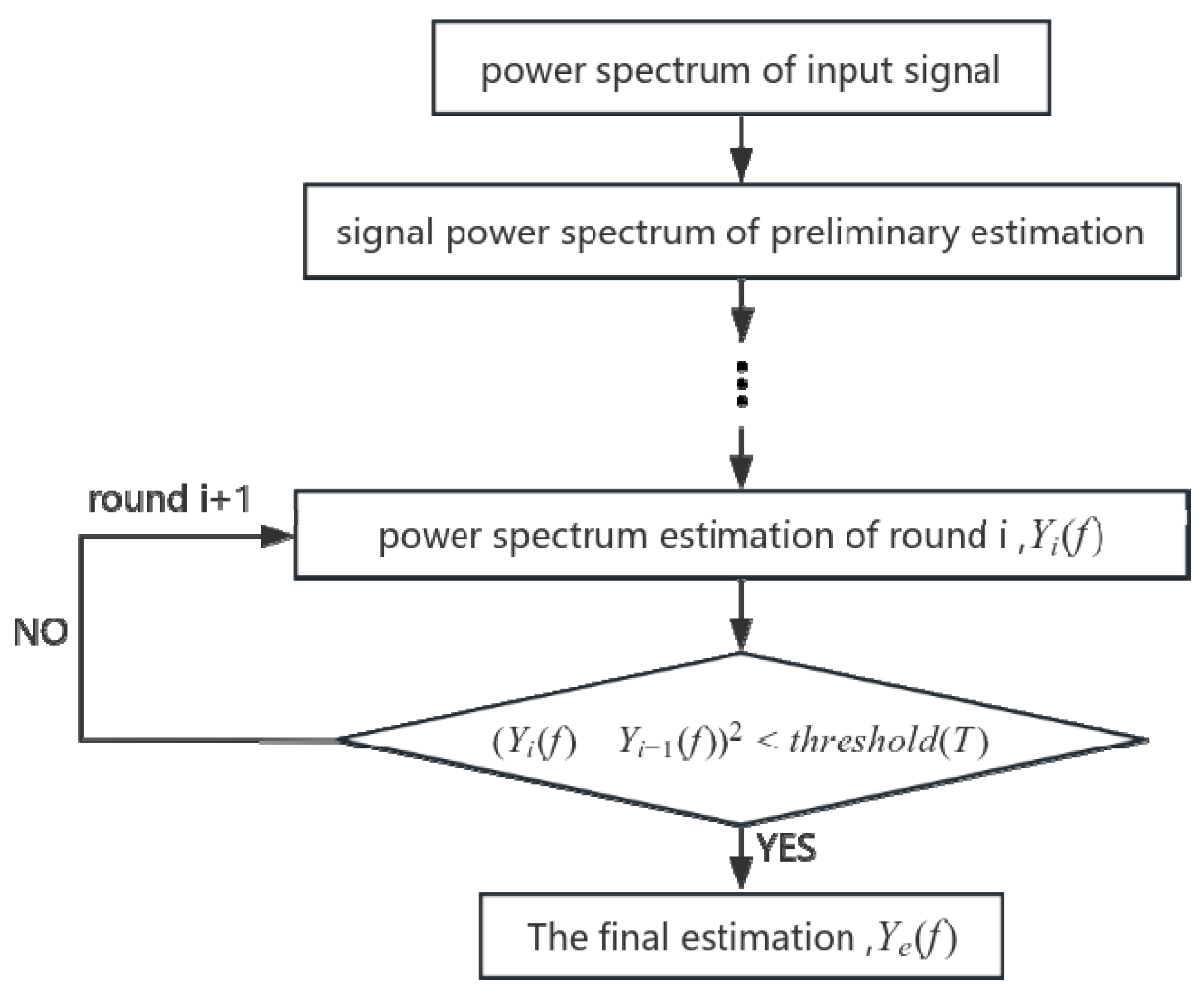
The SCCI algorithm obtains the final estimate of
through multiple iterations. For example, one iteration process consists of the following steps: (1) obtain the initial estimate of the signal power spectrum by applying the approximate model in Equation (1) to the input signal power spectrum; (2) identify the frequency points where the power values exceed the estimated power spectrum and set these values to the corresponding frequency point’s estimated power value, denoted as
, while keeping the power values at other frequency points unchanged, which forms a new signal power spectrum; and (3) apply the new signal power spectrum to the approximate model to obtain a new estimate of the signal power spectrum. Repeat the second and third steps iteratively until the iteration meets the threshold condition threshold (T). Due to the continuous elimination of jamming signal power, the estimated signal power spectrum approaches its true value. When the iteration stops, the final estimate of
is output. The iterative process is illustrated in
Figure 2.
The above process demonstrates that each iteration continuously reduces the jamming signal by eliminating the portion of jamming signal power greater than the power spectrum estimate obtained in the previous iteration. Through multiple iterations, the jamming signal component exceeding the true signal power spectrum is nearly eliminated, making the estimated signal power spectrum converge closer to the true values. Additionally, the iteration process in each round employs the gradient descent method, with the minimum variance between the input signal power spectrum and the estimated values from the approximation model as the criteria. This process iteratively determines the values of parameters a and b in each round.
3.2. Adaptive Variable Convergence Factor
The convergence factor used in the SCCME algorithm has a fixed value, which cannot simultaneously achieve fast convergence and a low steady-state error. The SCCI algorithm uses a hyperbolic tangent function to form an adaptive and variable convergence factor for the enhancing iterative performance effectively.
3.2.1. Parameter Settings
The error between the input signal power spectrum
and the model estimate
is defined as follows:
where N is the number of FFT points,
represents the estimated power spectrum of the input signal,
denotes the power spectrum of the signal, and the mean square error is provided by
The gradients of a and b can be obtained as follows:
Therefore, the updated formulas for a and b are provided by
In introducing the hyperbolic tangent function
and controlling the shape of the convergence curve through parameters α and λ, the relationship between the convergence factor and the error function is provided by
Simultaneously, due to the inevitable introduction of some noise in the error function
, the correlated values of the error
are used instead of
to suppress the impact of noise on the convergence performance. Substituting into Equation (8) yields Equation (9).
Equations (6) and (7) represent the iterative updated formulas for parameters a and b. Equation (9) introduces the adaptive variable convergence factor, which is influenced by parameter α to control the convergence speed. Parameter λ affects the shape of the function and achieves control over the convergence accuracy.
3.2.2. Analysis of the Parameters’ Impact on Performance
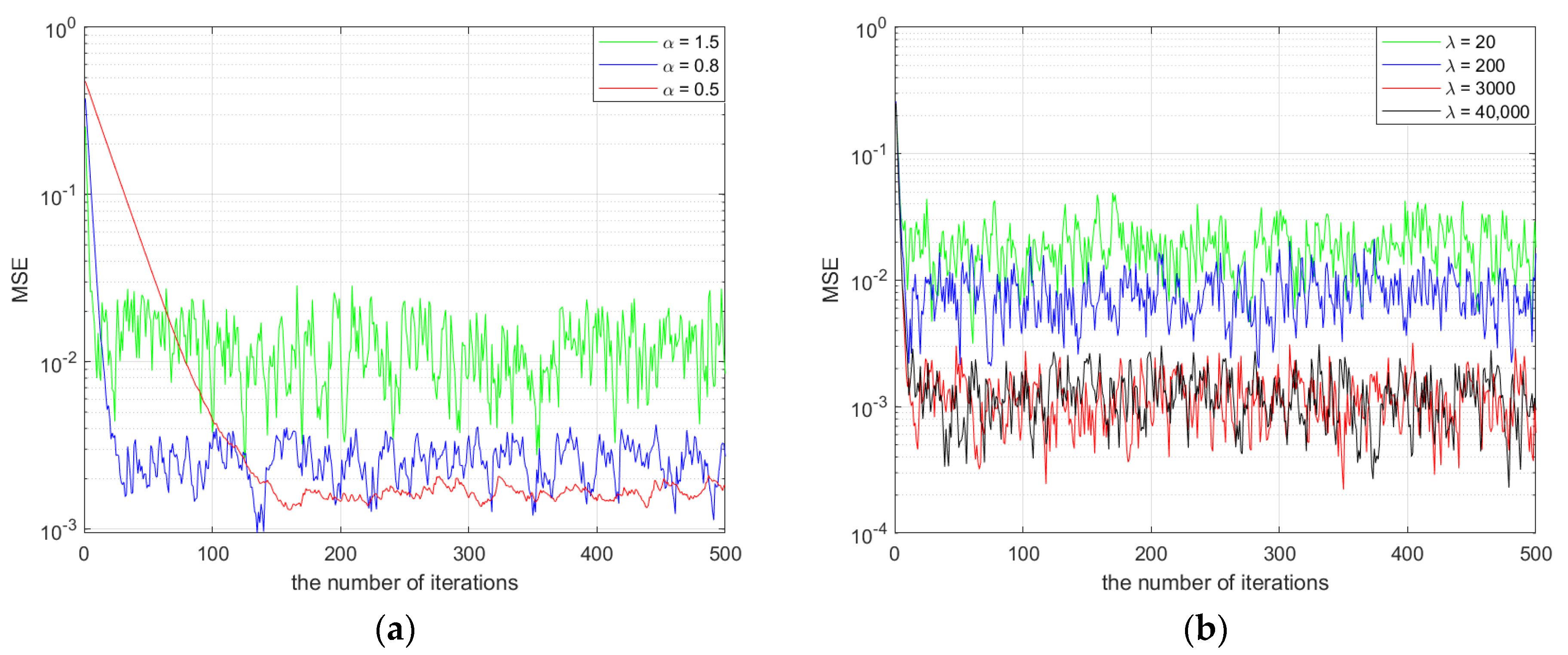
A simulation analysis of the impact of α and λ on the convergence performance in Equation (9) was conducted. In assuming that the input signal x(n) and noise v(n) are both zero-mean Gaussian white noise, with variances of 1 for x(n) and 0.01 for v(n), the system has a sampling point of 500, and each learning curve is the statistical average of 100 independent simulations. The learning curves for varying parameters α and λ are shown in
Figure 3.
Figure 3a shows the learning curves for α values of 0.5, 0.8, and 1.5 with λ set to 2000. Analyzing
Figure 3a, we can see that as α increases from 0.5 to 1.5, the algorithm’s convergence speed becomes faster, but the steady-state error also increases correspondingly. When α = 0.5, the algorithm reaches a steady state after about 150 iterations; when α = 1.5, it reaches a steady state after about 50 iterations, but with a larger steady-state error. Through simulation verification, the algorithm performs best when α is around 0.8.
Figure 3b shows the learning curves for λ values of 20, 200, 3000, and 40,000 with α set to 0.8. Analyzing
Figure 3b, we can see that as λ increases, both the steady-state error and the convergence performance of the algorithm gradually improve. When λ is set to 3000 or 40,000, the convergence speed and steady-state error are similar. To reduce the computational complexity of the system and improve the algorithm’s running speed, simulation verification shows that the algorithm performs best when λ is around 3000.
3.2.3. Performance Comparison of Algorithms
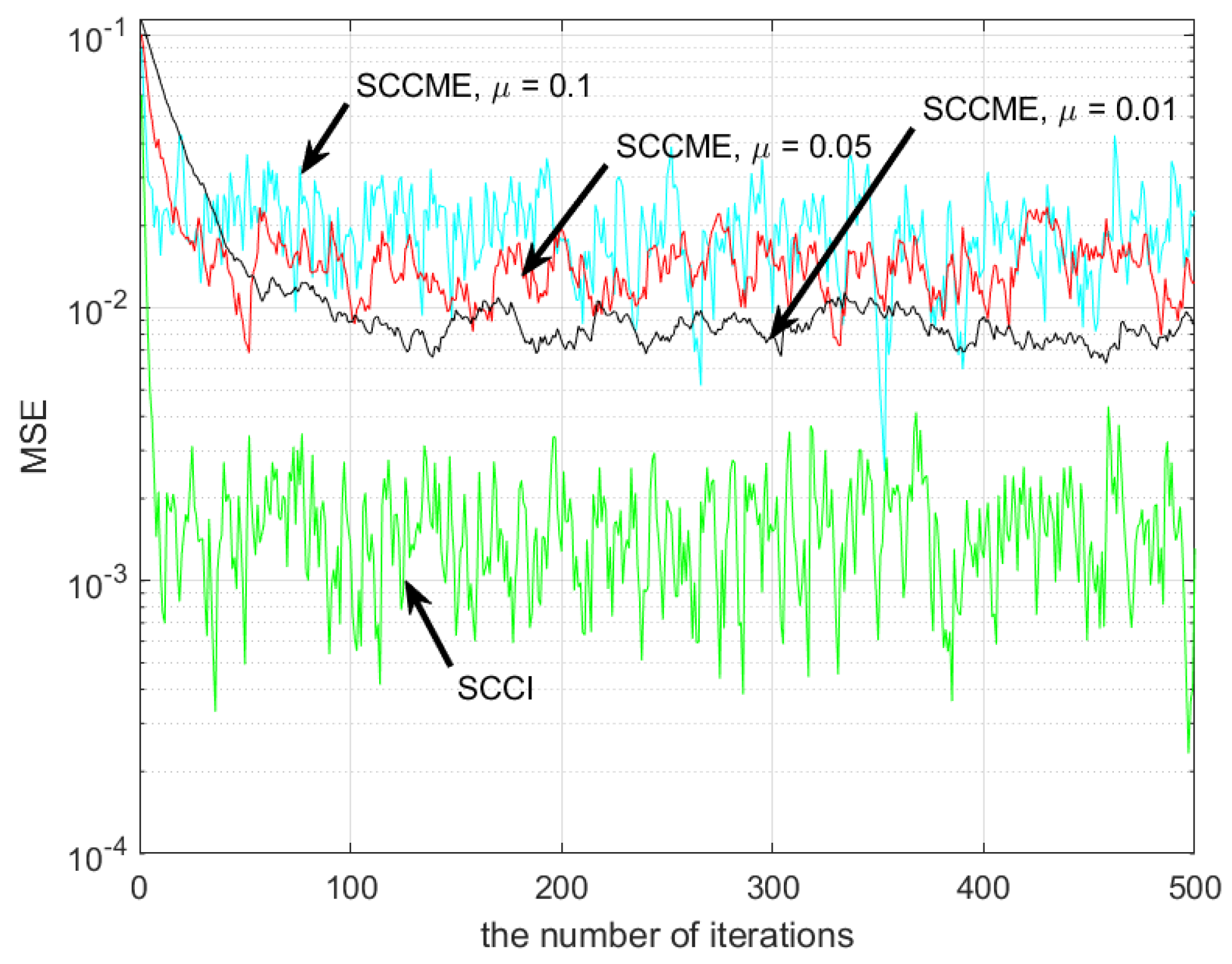
A comparison of the adaptive variable convergence factor in the SCCI algorithm with the fixed convergence factor in the SCCME algorithm was simulated. The system sampling points were 500, and each curve was the average result of 100 independent simulations. The fixed convergence factors in the SCCME algorithm were 0.1, 0.05, and 0.01, respectively. The simulation results are shown in
Figure 4.
From
Figure 4, it can be observed that the convergence speed and steady-state error performance of the SCCI algorithm are significantly higher than those of the SCCME algorithm with different convergence factor values. For the SCCME algorithm, the smaller the convergence factor value, the better the steady-state error performance, but the slower the convergence speed. Through the analysis above, it can be seen that compared to the SCCME algorithm with a fixed convergence factor, the SCCI algorithm has obvious advantages in convergence speed, a lower steady-state error, and stronger adaptability to external systems.
Here is a summary of the SCCI algorithm process, as shown in
Figure 5, with detailed steps outlined in
Table 1.
4. Simulation and Test Verification
To validate the effectiveness of the proposed algorithm, relevant simulations and experiments were conducted. Without loss of generality, an Iridium satellite system in LEO constellation was selected for both simulations and experiments as the signal radiation source. The Iridium system consists of Polar Earth Orbit satellites at an orbit height of 780 km, with a total of six orbital planes, each containing 12 satellites (including 1 backup satellite) [
41,
42]. The orbital inclination was 86.4°, and the orbital period was 100.13 min, providing global coverage. The Iridium system has duplex and simplex operational channels, with duplex channels operating in the frequency range of 1616.0–1626.0 MHz and simplex channels operating in the frequency range of 1626.0–1626.5 MHz. Additionally, Iridium satellites achieve channel and time division by controlling the transmitted spot beams, enabling FDMA/TDMA/SDFA/TDD multiplexing for users [
43]. Furthermore, the downlink transmission signal structure of the Iridium satellite primarily includes pilot signals and BPSK and QPSK modulation schemes. Users can receive signals from the seventh channel every 4.32 s.
4.1. Simulated Test
For the simulation experiments, the signal used a down-converted Iridium intermediate frequency (IF) simulated signal with a center frequency of 270,833 Hz. The jamming signal was modeled as Gaussian band-limited noise with a mean of 0 and a variance of 1.
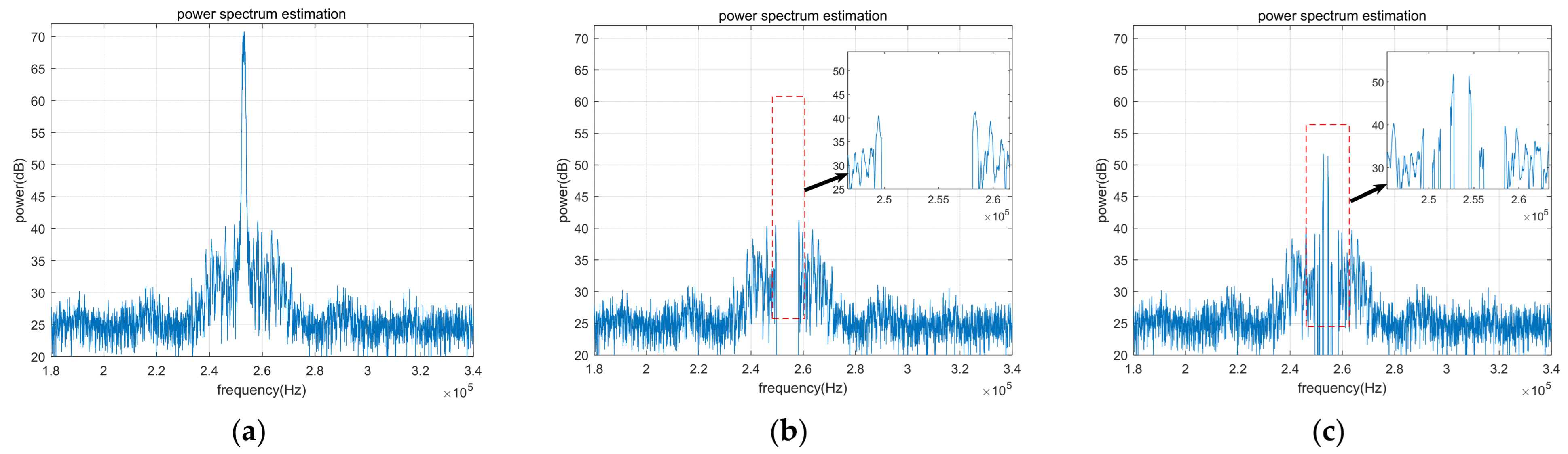
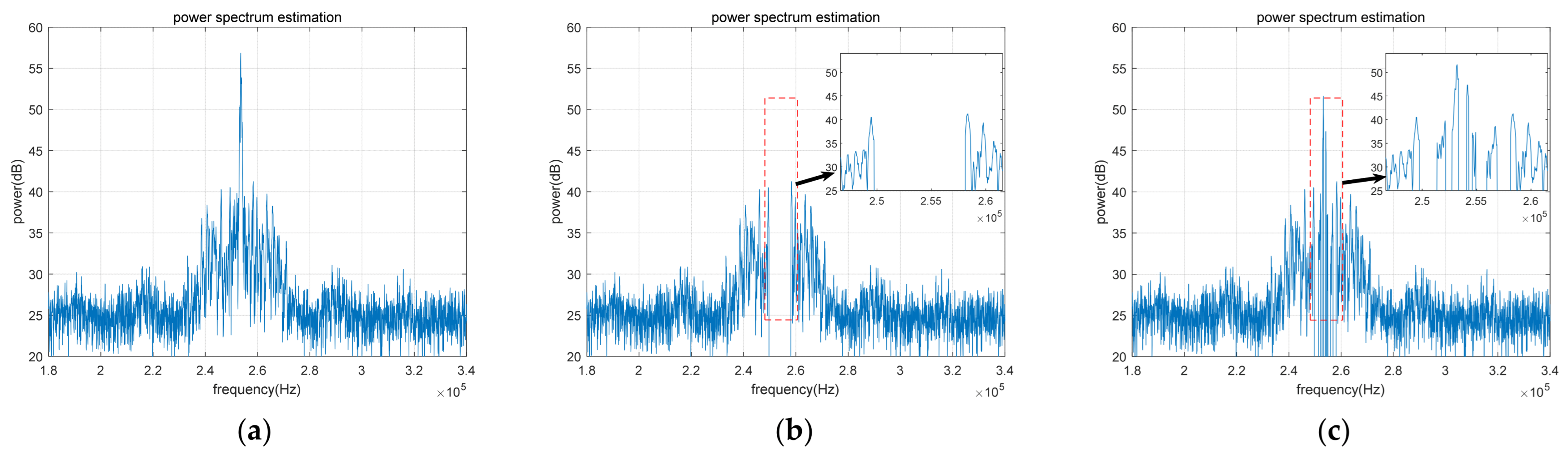
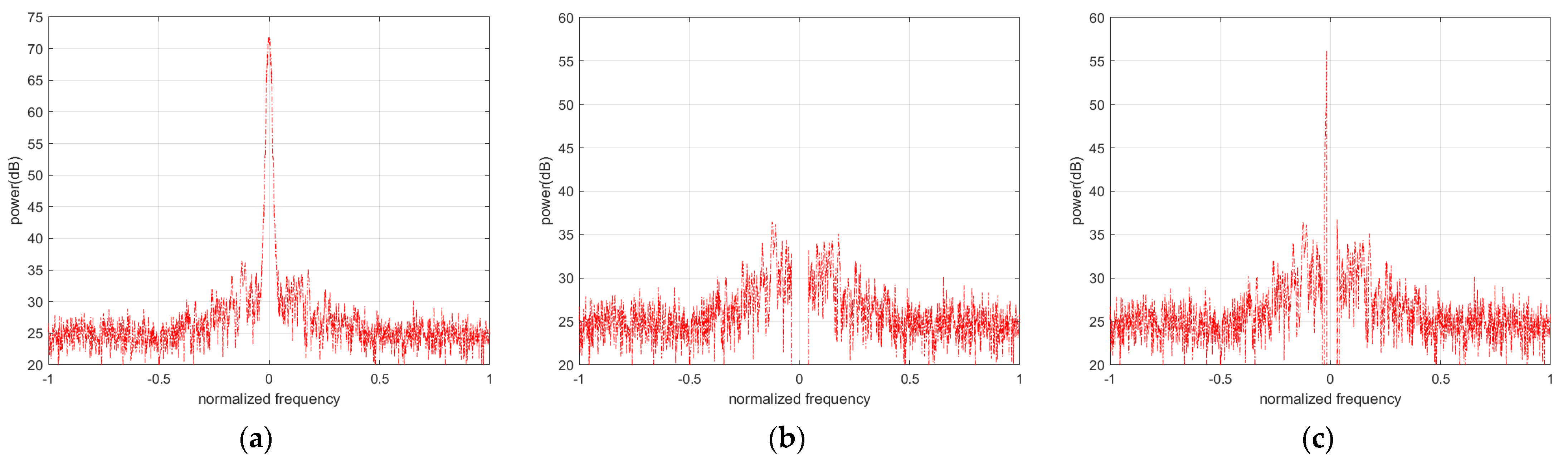
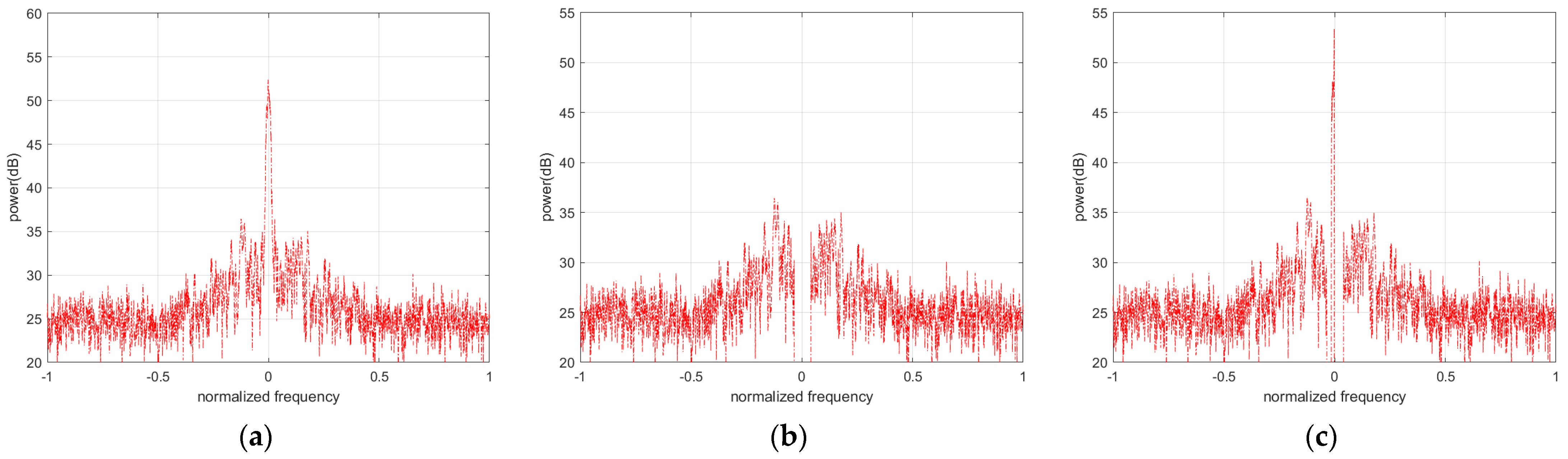
4.1.1. Signal Power Spectrum Simulation before and after Anti-Jamming
Firstly, changes in the power spectrum before and after jamming suppression were analyzed to verify the algorithm’s jamming suppression capability. Two scenarios were designed: a strong jamming signal with a Jamming-to-Signal Ratio (JSR) of 30 dB and a weak jamming signal with a JSR of 15 dB. The jamming signal bandwidth was set to 40 kHz in both scenarios.
From
Figure 6 and
Figure 7, it can be observed that, in the LEO satellites signal scenario, the SCCME algorithm consistently exhibited poor anti-jamming effects, with the interference spectral lines not completely suppressed. This poor performance may be due to errors in the estimation model, leading to a smaller detection probability and, consequently, residual interference spectral lines. By contrast, the SCCI algorithm completely suppressed the interference spectral lines.
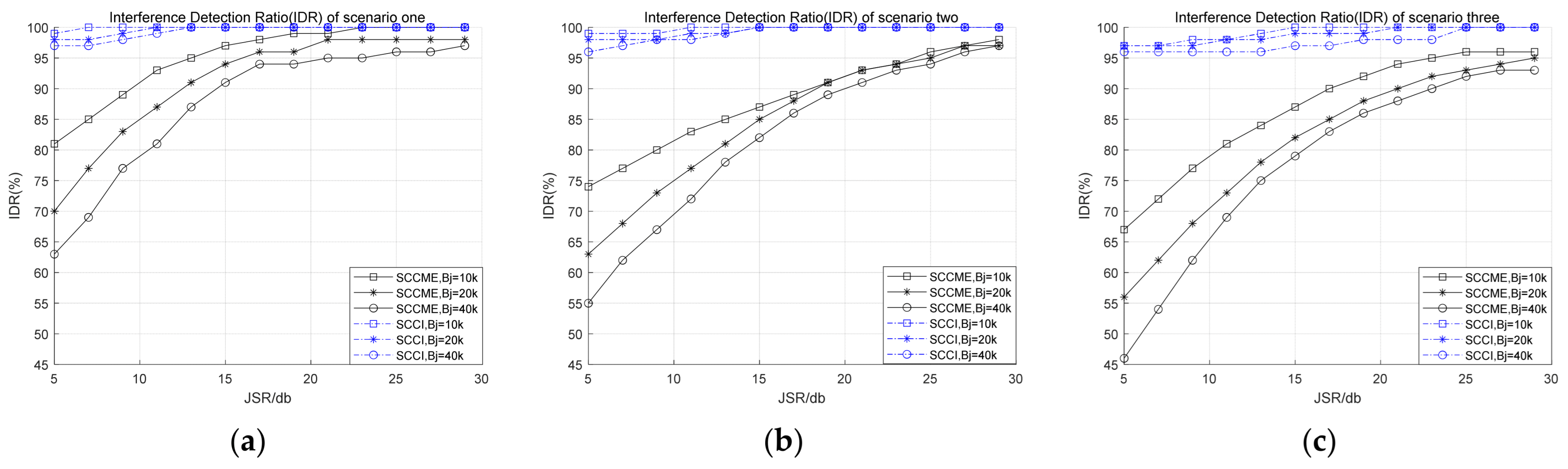
4.1.2. Simulation of Interference Detection Performance for Anti-Jamming Algorithm
The next step involves validating the effectiveness of the proposed algorithm’s interference detection performance. Three experiments were designed to compare the interference detection performance under different conditions of jamming center frequency offset from the signal center frequency and bandwidth. For this purpose, we defined the interference detection ratio (IDR), denoted as
, to measure the interference detection performance, where
is the number of detected interference spectral lines, and
is the total number of interference spectral lines. The specific simulation parameters are provided in the
Table 2.
Figure 8 shows the interference spectral line detection rate under different JSRs. The horizontal axis represents the JSR, and the vertical axis represents the interference spectral line detection rate.
Figure 8 demonstrates the following. (1) For the SCCME algorithm, the farther the jamming center frequency is from the carrier, and the wider the jamming signal bandwidth, the lower the interference detection probability and the greater the impact of the model’s estimation error on interference detection. (2) In different scenarios, the interference detection rate of the SCCI algorithm was consistently >96%, indicating that the algorithm is insensitive to the center frequency of the jamming signal.
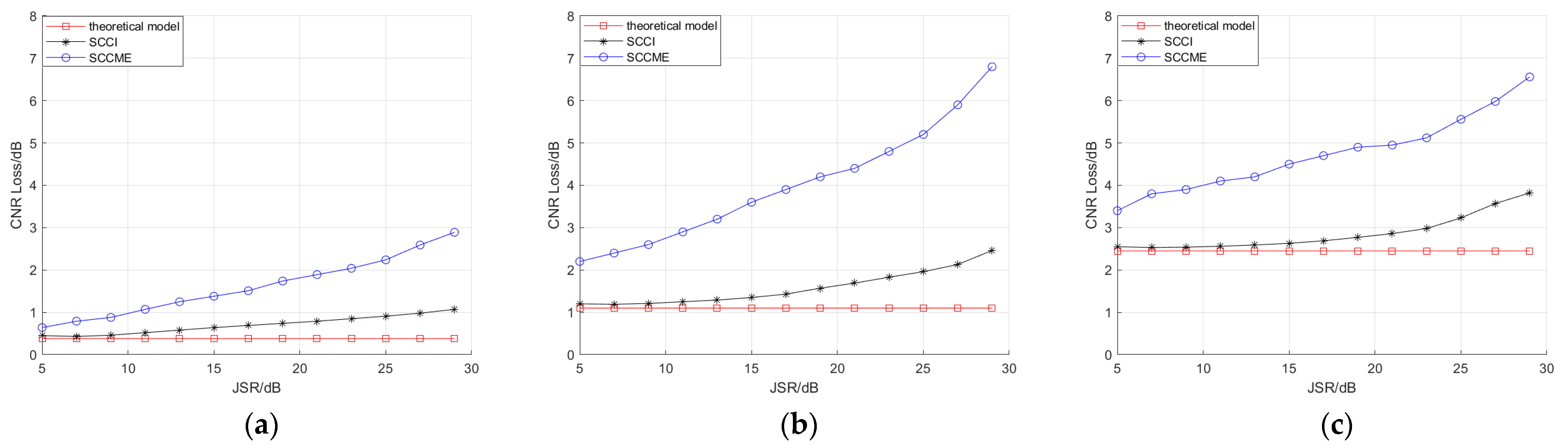
4.1.3. Verification of Anti-Jamming Performance
The anti-jamming performance comprehensively considers anti-jamming loss and interference suppression capability, using the quality of the signal after anti-jamming as the evaluation target. Therefore, the CNR loss was used as the measure of the anti-jamming performance to verify the anti-jamming performances of different algorithms, defined as
, where
is the CNR of the input signal, and
is the CNR of the output signal from the anti-jamming module. In the simulation, the frequency domain anti-jamming theoretical loss was used as a reference. If the interference is completely suppressed, the CNR loss introduced by frequency domain anti-jamming can be calculated as follows: [
44]
where
is the bandwidth of the receiver’s front-end filter,
is the normalized signal power spectral density, and the power spectral density of the frequency domain anti-jamming filter is
. The frequency domain response of the anti-jamming filter is
where
is the jamming signal center frequency, and
is the jamming signal bandwidth.
A simulation analysis of the anti-jamming performances of different algorithms was performed, and the specific experimental parameter settings were as shown in
Table 3.
Figure 9 shows the simulation results for different scenarios, with the horizontal axis representing the jamming signal bandwidth and the vertical axis representing the CNR loss.
The simulation results indicate that the CNR loss of the SCCI algorithm after interference suppression is within 2 dB of the theoretical value, while the SCCME algorithm consistently exhibits a significantly higher CNR loss.
4.2. Actual Experimental Verification
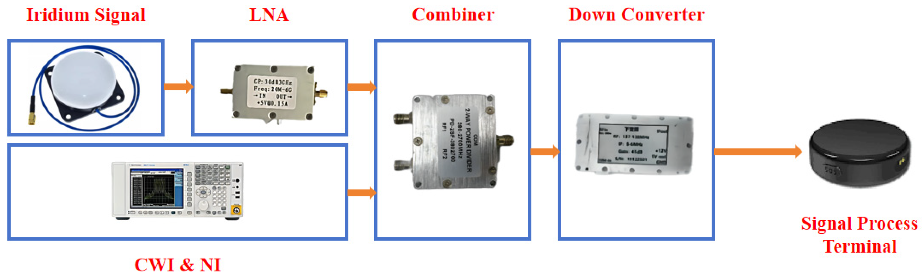
In the above simulation experiments, the improved jamming suppression performance of the SCCI algorithm compared to the SCCME algorithm was verified. To further evaluate this algorithm’s effectiveness, actual signal anti-jamming experiments were conducted on the rooftop of a new main building at Beihang University using a hardware platform, as shown in
Figure 10. The system uses a dedicated Iridium antenna to collect signals. Gaussian jamming generated by the signal source was combined with the Iridium signal through a hybrid coupler. The combined signal was then frequency-shifted to an intermediate frequency (IF) using down-conversion devices. Finally, the signal was processed through a signal reception and processing platform using different anti-jamming processing algorithms for performance comparisons. As shown in
Figure 11, the top curve indicates that during the test period, a total of four Iridium satellites were visible. The constellation map corresponding to the visible epochs of the Iridium satellites is shown in
Figure 11.
The experiment involved setting different levels of jamming signal using a signal source and designing scenarios with strong jamming (JSR 35 dB) and weak jamming (JSR 15 dB). The jamming signal bandwidth was set to 40 kHz.
Figure 12 and
Figure 13 show the results of the anti-jamming algorithm under different jamming scenarios.
The experimental results further validate the effectiveness and jamming suppression performance of the SCCI algorithm in the LEO satellites signal scenario, whereas the SCCME algorithm consistently exhibited poor anti-jamming effects with incomplete suppression of interference spectral lines.
6. Conclusions
In the past few decades, with the development of drone technology, its applications have become increasingly widespread. However, faced with adverse electromagnetic environments such as urban multipath jamming and intentional jamming, traditional GNSS positioning technology has gradually revealed many issues, threatening the performances of drones in harsh environments. Applying LEO satellite SOP positioning technology to drone positioning has become an important option for drone development. However, due to characteristics such as the high SNR and narrow downlink bandwidth of LEO satellite signals, which differ significantly from navigation signals, traditional anti-jamming achievements cannot be directly applied, especially for the time–frequency domain anti-jamming scenarios of single antennas widely used in the drone field. Therefore, researching anti-jamming algorithms for drone LEO satellite SOP positioning has significant practical value. This research proposes the SCCI algorithm for LEO satellite constellation signals. This algorithm significantly reduces errors generated during model fitting. Additionally, an adaptive variable convergence factor was designed to balance fast convergence and low steady-state error during iterations. In considering parameters such as jamming signal bandwidth, center frequency, and intensity, the algorithm was tested using signals from the Iridium constellation in simulations and experimental data processing. Compared to those of traditional algorithms, the results demonstrate that the proposed algorithm improves the effectiveness of jamming threshold settings and the jamming suppression performance under narrow bandwidths and high-power conditions. In the context of LEO satellite anti-jamming scenarios, the algorithm notably enhances the frequency domain anti-jamming performance. This holds high application value for drone positioning scenarios.


 ,
, 


