
Early Drought Detection in Maize Using UAV Images and YOLOv8+
1
College of Information Science and Technology, Gansu Agricultural University, Lanzhou 730070, China
2
Key Laboratory of Opto-Technology and Intelligent Control, Ministry of Education, Lanzhou Jiaotong University, Lanzhou 730070, China
3
College of Forestry, Gansu Agricultural University, Lanzhou 730070, China
4
Intelligent Sensing and Control Laboratory, Shandong University of Petrochemical Technology, Dongying 257000, China
*
Author to whom correspondence should be addressed.
Drones 2024, 8(5), 170; https://doi.org/10.3390/drones8050170
Submission received: 22 March 2024
/
Revised: 22 April 2024
/
Accepted: 23 April 2024
/
Published: 24 April 2024
(This article belongs to the Special Issue Application of Uncrewed Aerial Vehicles (UAVs) in Vegetation Monitoring)
Abstract
:The escalating global climate change significantly impacts the yield and quality of maize, a vital staple crop worldwide, especially during seedling stage droughts. Traditional detection methods are limited by their single-scenario approach, requiring substantial human labor and time, and lack accuracy in the real-time monitoring and precise assessment of drought severity. In this study, a novel early drought detection method for maize based on unmanned aerial vehicle (UAV) images and Yolov8+ is proposed. In the Backbone section, the C2F-Conv module is adopted to reduce model parameters and deployment costs, while incorporating the CA attention mechanism module to effectively capture tiny feature information in the images. The Neck section utilizes the BiFPN fusion architecture and spatial attention mechanism to enhance the model’s ability to recognize small and occluded targets. The Head section introduces an additional 10 × 10 output, integrates loss functions, and enhances accuracy by 1.46%, reduces training time by 30.2%, and improves robustness. The experimental results demonstrate that the improved Yolov8+ model achieves precision and recall rates of approximately 90.6% and 88.7%, respectively. The mAP@50 and mAP@50:95 reach 89.16% and 71.14%, respectively, representing respective increases of 3.9% and 3.3% compared to the original Yolov8. The UAV image detection speed of the model is up to 24.63 ms, with a model size of 13.76 MB, optimized by 31.6% and 28.8% compared to the original model, respectively. In comparison with the Yolov8, Yolov7, and Yolo5s models, the proposed method exhibits varying degrees of superiority in mAP@50, mAP@50:95, and other metrics, utilizing drone imagery and deep learning techniques to truly propel agricultural modernization.
1. Background
Against the backdrop of escalating global climate change, agriculture faces increasingly severe drought threats. Among them, maize, one of the world’s important staple crops, is significantly impacted by drought during its seedling stage, affecting both yield and quality. As the crop with the widest planting area and highest total output in China, maize plays a crucial role in China’s food security and feed supply. The growth of crops relies on the supply of water and nutrients, and the efficiency of their utilization directly impacts maize yield. However, due to the lack of precise predictions of water and fertilizer requirements, the quantitative management of water and fertilizer in field planting lags behind [1]. In some regions, the use of unreasonable irrigation amounts not only wastes water resources but also affects the growth and quality of maize. Additionally, in the context of large-scale mechanized farming, traditional manual inspection methods are clearly unable to meet the demand for the efficient and rapid monitoring of large-scale farmland.
With the continuous development of artificial intelligence and information technology, various deep learning technologies have been widely applied in the detection of drought stress in maize. Utilizing drones to capture high-resolution RGB images and multispectral data during aerial photography, combined with deep learning algorithms, enables the rapid and accurate analysis and diagnosis of the health status of maize seedlings. Meanwhile, remote sensing technology provides more extensive spatial information and data support. By integrating drones and deep learning technologies, the comprehensive monitoring and evaluation of early-stage drought in maize can be achieved [2]. The application of drones and deep learning technologies in the detection of drought stress in maize seedlings not only improves detection efficiency and accuracy, and reduces the impact of drought on maize yield, but also provides a scientific basis for farmland management decisions, promoting the sustainable and modernized development of agricultural production. Drones and deep learning technologies have broad prospects for application in the detection of drought stress in maize.
The Hexi Corridor in Gansu, China, situated at 100.82° E and 38.43° N, experiences a continental desert grassland climate characterized by abundant sunlight, scarce rainfall, vast land area, low population density, and a thriving animal husbandry industry. Sun protection measures are essential for agricultural activities in this region. Green storage corn, with an average mature height of 3.16 m, serves as a crucial feed source for livestock, supporting the development of the animal husbandry sector. In maize fields, drip irrigation lines are installed beneath each row of maize, and the soil is covered with a black plastic film. This setup aims to reduce evaporation and ensure that crops receive an ample supply of water. Drought can severely affect both the yield and quality of maize, a crucial food crop, particularly when drought conditions occur during the seedling stage. Hence, there is a pressing need to develop an integrated, real-time, high-precision, automated processing, and data-rich detection model for early drought detection in maize.
2. Introduction
Early drought detection in maize can be achieved using a variety of methods, including ground patrols, soil moisture monitoring, remote sensing technology, as well as machine learning and deep learning technologies. Ground patrols involve manually observing the morphology, color, and growth of maize leaves to check for symptoms of drought stress, such as leaf curling and discoloration. However, this method suffers from the drawbacks of significant subjective influence and high manual workload. Soil moisture monitoring utilizes sensors or other monitoring devices to continuously monitor the moisture content in the soil in real time, determining if the soil is experiencing water shortages. Although this method provides real-time data, it is costly and cannot comprehensively cover all areas.
2.1. Research Work by Relevant Scholars
In terms of remote sensing technology for early drought detection in maize, Liu et al. [3] (2011) explored the response of maize leaf temperature to drought using infrared thermography and identified quantitative trait loci (QTLs) related to drought tolerance through genetic mapping, providing a genetic basis and tools for breeding drought-tolerant maize. Mertens et al. [4] (2021) demonstrated the utility of hyperspectral imaging in an automated plant phenotyping platform, enabling the high-resolution monitoring of physiological characteristics. Through innovative spectral measurement and processing methods, they effectively detected changes in maize reflectance and physiology under day–night cycles, development, and drought induction. Brewer et al. [5] (2022) utilized drone optical and infrared thermography combined with random forest machine learning algorithms to accurately estimate maize leaf temperature and stomatal conductance, providing smallholder farmers with an important early warning system to optimize irrigation planning and decision-making processes. The research conducted by Pradawet et al. [6] (2023) in Phitsanulok Province, Thailand, enhanced the effectiveness of thermal infrared imaging in detecting maize water stress and predicting yield losses under drought conditions through a novel Crop Water Stress Index (CWSI) method, validated in controlled and field conditions. Praprotnik et al. [7] (2023) proposed a method for testing hyperspectral imaging for the early detection and differentiation of biotic and abiotic stresses in maize, showing that hyperspectral imaging can detect nematode infestations and drought stress early. Despite the excellent performance of these methods in terms of accuracy and reliability, they have drawbacks, such as high imaging equipment costs, complex data processing and analysis, and significant susceptibility to weather conditions. Additionally, the lack of portability due to varying measurement baselines for the same crop in different locations and at different times poses a challenge.
Machine learning and deep learning technologies have shown significant potential in early drought detection in maize. Jiang et al. [8] (2018) proposed a computer vision-based maize drought detection method, which built a model from aspects including color, texture, and plant morphology, achieving a recognition rate of 98.97%. Zhuang et al. [9] (2018) established a maize plant early water stress detection model using outdoor cameras and image analysis, achieving detection accuracies of 80.95% and 90.39% under different water treatment conditions, demonstrating a good detection performance in the maize field. An et al. [10] (2019) presented a maize drought identification and classification method based on deep convolutional neural networks (DCNNs), achieving accuracies of 98.14% and 95.95% in drought stress identification and classification, respectively. Goyal et al. [11] (2024) proposed a customized convolutional neural network for in situ maize drought stress identification and classification, achieving accuracies of 98.71% and 98.53% on the training and test sets, respectively, surpassing the latest technology architecture with 0.65 million parameters. Transfer learning with ResNet50 and EfficientNetB1 achieved accuracies of 99.26% on the test set. These methods can efficiently process and analyze data, enabling the precise identification of maize plants under drought stress and the accurate assessment of drought severity. However, they require a large amount of high-quality data for algorithm training, as well as tuning by professional personnel and model optimization, resulting in high maintenance costs.
Furthermore, in the aspect of target detection for unmanned aerial vehicles (UAVs), Fu et al. [12] (2023) proposed a novel target detection model named Efficient YOLOv7-Drone. This model aims to address the efficiency and accuracy issues of target detection in aerial images captured by low-cost small rotary-wing UAVs. Pu et al. [13] (2024) presented a new corn tassel detection model named Tassel-YOLO in this study. By introducing a global attention mechanism, GSConv convolution, and VoVGSCSP module based on YOLOv7, and improving the loss function to the SIoU loss function, a high accuracy and real-time performance for the corn tassel detection task were achieved. Wang et al. [14] (2024) proposed a novel deep learning network named YOLO-DCAM. Based on YOLOv5, the effective detection of individual trees in complex scenes was achieved by reasonably introducing deformable convolution layers and efficient multi-scale attention modules. This provides important support for precise and scientific forest management.
2.2. Contribution of This Article
Based on the research efforts of the scholars mentioned above and the practical background of this study, we propose a novel early drought detection method for maize utilizing unmanned aerial vehicle (UAV) images and Yolov8+. The summary diagram of this article is shown in Figure 1. The main contributions of this article are as follows:
(1) In the arid and sunny climate of the Gansu Hexi Corridor in China, characterized by a continental desert grassland climate with minimal rainfall, a novel data augmentation method was developed. This method involved the selective removal of colors from the original images that tend to interfere with the identification of the corn’s green area, such as those produced by the plastic film, soil, shadows, and intense light. By retaining only the green area of the corn, the clarity and effectiveness of the model’s drought detection capabilities were enhanced for improved observation and analysis.
(2) In this study, a new deep learning model, Yolov8+, was investigated. The Backbone component of the model utilized the C2F-Conv module to optimize the parameters and computational cost, resulting in a reduction in the model’s deployment cost [15]. Additionally, the inclusion of a CA attention mechanism module enhanced the model’s performance for unmanned aerial vehicle target monitoring. This module effectively captured small feature information in images and addressed the challenge of sparse feature information across various drought categories.
(3) In the Yolov8+ model, the Neck component incorporates a BiFPN fusion architecture and spatial attention mechanisms to overcome the challenge of inadequate long-distance information propagation in object detection. This design enhancement boosts the model’s capability [16] to detect small and obscured targets, showcasing superior performance in real-world scenarios. Additionally, the Head component was expanded to produce a 10 × 10 output. Through the integration of loss functions, the precision was improved by 1.46%, training time was reduced by 30.2%, and overall robustness was enhanced.
(4) The enhanced Yolov8+ model architecture and optimized strategy demonstrated exceptional performance, achieving remarkable mAP@50 and mAP@50:95 values of 89.16% and 71.14%, respectively. The speed of drone image detection using this model was 24.63 ms, with a compact model size of 13.76 MB.
3. Experimental Data
3.1. Data Collection
The data samples were collected from the experimental field of the Research and Development Center of Huarui Ranch in Gansu, China, with geographic coordinates precisely at 100.82° E and 38.43° N. The region has a continental desert grassland climate, characterized by arid conditions, low rainfall, and abundant sunlight. The data sample images were collected using the Samsung GW1 mobile shooting equipment and DJI Mavic Classic 3 drone. The Samsung GW1 sensor features high light sensitivity, low noise, and excellent color reproduction, making it suitable for daily small-scale data collection. A total of 400 images were collected with a resolution of 4640 × 2608 pixels and a file size of approximately 5.5 MB. The drone flew at a height of 5 m above the experimental field every day at noon to capture the images. As shown in Figure 2, the corn plants are distributed in rows of two, with a spacing of 1 m between rows, 25 cm between the two rows, and a distance of 20 cm between the roots of two corn plants. A total of 1600 images were collected from the drone shots, with a resolution of 5280 × 2970 pixels and a file size of approximately 15.8 MB. Various methods, including super-green factor segmentation, image binarization, and Sobel operator edge extraction, were used to enhance the image transformation of the collected corn seedling pictures and improve the effectiveness of data image collection.
3.2. Data Categories and Datasets
Under drought conditions, the leaf morphology of maize seedlings may undergo noticeable changes. Typically, plants affected by drought stress adopt a series of adaptive measures to reduce water evaporation and enhance water use efficiency. Specifically, as shown in Figure 3, maize seedlings under early drought stress exhibit sharp leaf tips, relatively neat leaf margins, and no obvious damage or irregular edges. Seedlings under semi-drought conditions display rounded leaf tips and margins compared to the upper leaves, along with undulating leaf edges and an overall wider appearance. Maize seedlings under optimal conditions exhibit simpler leaf contours, rounded leaf tips and margins, and the widest width.
In this study, the rectangle labeling tool LabelImg (version 1.8.6) was utilized for the manual annotation of the collected maize images. The annotation process involved labeling the images with category and location information, including three categories: drought, semi-arid, and optimal. Subsequently, the annotated information was saved as a .txt file, thus finalizing the construction of the dataset. To enhance the model’s ability to accurately identify maize seedlings under varying drought levels, the images were partitioned into training, validation, and testing sets in an 8:1:1 ratio [17]. Given the challenges associated with distinguishing drought levels in maize seedlings based on subtle features, in addition to data augmentation techniques (Mosaic, Affine, Perspective, Hsv) integrated into Yolov8, various methods were employed, such as super-green factor segmentation, image binarization, and Sobel edge detection, combined with hyperspectral image fusion. These approaches were implemented to ensure the diversity of the collected data images, ultimately aiming to improve network training efficiency, minimize model memory consumption, and boost the generalization capability of the model.
3.3. A800 Computing Server
The computational resources employed in this study were provided by the Intelligent Sensing and Control Laboratory at Shandong University of Petroleum and Chemical Technology. The hardware components consisted of the NF5468M6 server manufactured by Inspur. The server configuration included 128 GB of memory, an Intel Xeon(R) Silver 4314 CPU @ 2.4 GHz × 64 processor, 8 NVIDIA A100 GPUs, a graphics renderer of llvmpipe (LLVM 7.0, 256 bits), and a storage disk capacity of 2 TB. The software environment utilized in this study comprised Python version 3.9, PyTorch version 2.0, CUDA version 11.7, Linux kernel version 3.10.0-1127.el7.x86_64, and GNOME version 3.28.2.
4. YOLOv8 Network Model
4.1. YOLOv8 Model
The significant contributions of YOLOv8 can be categorized into two primary aspects: firstly, it demonstrates remarkable performance in terms of detection accuracy; secondly, it embraces a novel design framework devoid of anchor boxes [18]. In comparison to its predecessors, namely YOLOv3, YOLOv4, and YOLOv5, YOLOv8 presents fewer innovative alterations in its components, with the majority of components inheriting the architecture of YOLOv5. The architecture of YOLOv8 is segmented into three distinct parts: Backbone, Neck, and Prediction, as depicted in Figure 4. Within the Backbone segment, the C3 module in YOLOv5 is supplanted by a sole C2F module, while the other modules predominantly maintain consistency with YOLOv5. The Neck section also integrates the PANet configuration, streamlining the top-to-bottom connection with two C2Fs, alongside the retention of two C2Fs and two CBSs for the left and right connections, respectively, thereby further simplifying the structure of the Neck section.
The Head section undergoes notable transformations, integrating 12 CBSs and 6 Conv layers. In the Neck section, three sets of features are produced in total, each set branching into two pathways upon entering the Head: one pathway is dedicated to the computation of detection boxes, with 64 feature channels feeding into the Anchor module to generate these boxes; the other pathway focuses on computing the probabilities of each class, with 80 feature channels passing through the sigmoid activation function to yield the probabilities associated with 80 respective classes. Subsequently, the detection boxes and class probabilities are combined, resulting in a total of 84 feature channels [19]. Three feature maps are generated from bottom to top, with dimensions of 80 × 80 × 80, 40 × 40 × 40, and 20 × 20 × 20.
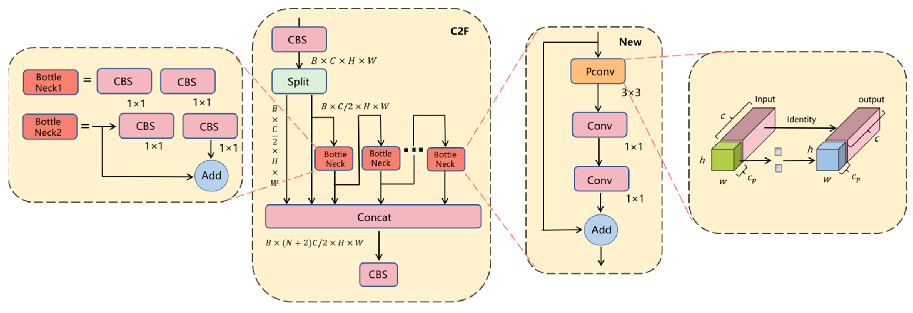
After the input of the C2F module undergoes processing via a CBS, the output dimensions are transformed into B, C, H, and W, where B denotes the number of images, C indicates the number of channels, and H and W represent the height and width of the feature map, respectively [20]. The detailed structure is depicted in Figure 5. During the Split operation, the channels are divided into two segments, with C/2 channels assigned to each segment. The channels in the left segment are directly outputted, whereas the channels in the right segment are split into two branches. One branch is directly outputted, while the other branch undergoes further splitting by a BottleNeck into two branches. One branch is directly outputted, while the other branch is split again by the subsequent BottleNeck. Essentially, the output of each BottleNeck must be preserved and utilized as input for the following BottleNeck. Eventually, all corresponding feature channels are fused, resulting in dimensions of B × (N + 2)C/2 × H × W.
In this architecture, the outputs of the left and right branches, along with the outputs of N BottleNeck, are amalgamated, totaling N + 2 BottleNeck, and ultimately conveyed through a CBS. In contrast to the C3 module, the C2F module necessitates the aggregation of outputs from all BottleNeck, consequently enhancing feature utilization [21]. Nonetheless, the input channel count of the C2F module experiences a notable escalation, thereby resulting in a further augmentation in computational complexity.
4.2. Anchor Module without Anchor Boxes
The Anchor module is composed of two components: GAP (Global Average Pooling) and Grid. In Figure 5 above, the input of 64 × 20 × 20 undergoes processing by the Anchor module to yield an output of 16 × 4 × 400. Within this module, SoftMax is employed to normalize the 16 feature channels. This is followed by convolutional calculations, where Conv weights are constrained between 0 and 15, and the GAP dimensions are 4 × 400. The Grid corresponds to the centers of the grid structure, with flattened dimensions of 2 × 400. By utilizing both GAP and Grid, the pertinent information for detection boxes can be computed effectively.
Specifically, the coordinates of the upper left corner of the detection box, bx1, by1, etc., are equal to the coordinates of the center point (x, y) minus x1, y1, and the coordinates of the lower right corner, bx2, by2, etc., are equal to the coordinates of the center point (x, y) plus x2, y2. Therefore, the detection box corresponding to each feature point on the feature map can be obtained, which is the design idea of the Anchor module without the need to pre-set anchor boxes.
5. Yolov8+ Network Model
5.1. Lightweight C2F-Pconv Module
The C2F module within the Backbone of the YOLOv8 model is noted for its exceptional performance. However, as the number of channels increases, there is a corresponding escalation in computational complexity. To address challenges encountered when dealing with small-to-medium-sized targets, particularly in drone applications where issues such as excessive target quantity and limited computing power may arise, resulting in system lag, overheating, false alarms, and missed detections, we propose a solution. In order to alleviate these challenges and lower model deployment costs, we advocate for the replacement of the original C2F module with an enhanced C2F-Pconv module [22].
Current lightweight networks, such as MobileNet and GhostNet, commonly employ depth-wise convolution or group convolution to extract spatial features, thereby reducing floating-point operation counts (FLOPs). However, these operators may lead to increased memory access, resulting in inefficient fragmented computation. In contrast, the Pconv module utilized in FasterNet specifically targets redundant information within feature maps. By performing regular convolutions on specific channels while leaving others unaffected, the Pconv module effectively harnesses device computing capabilities, reducing redundant information and memory access for improved efficiency.
Here, h and w represent the height and width of the feature map, respectively; c represents the number of input channels; cp represents the number of channels [23] involved in convolution; k denotes the kernel size; and r denotes the convolution rate. The computational complexity expression for FPConv is shown in Equation (1), while the calculation expression for memory access Mac is shown in Equation (3).
The concatenated BottleNeck modules have been instrumental in facilitating the extraction and fusion of features at various scales to enhance the expressive capability of feature maps. However, within the YOLOv8 framework, an excessive reliance on BottleNeck structures can lead to an escalation in the computational burden. Taking cues from the efficient Pconv module in FasterNet, this study proposes a novel BottleNeck structure, as depicted in Figure 6, to replace the feature extraction process within the C2F module. Through the use of class inheritance, the newly designed BottleNeck module is intended to serve as the principal gradient flow branch, with the goal of reducing floating-point operations and the computational load within the model. Additionally, it aims to decrease memory consumption and alleviate the strain on computational resources.
In the case of distant maize seedlings, feature information is often sparse and distributed across three distinct categories: drought, semi-arid, and optimal conditions. To address this challenge, this study proposes the integration of a lightweight attention mechanism, referred to as Coordinate Attention (CA), during the feature extraction phase. The CA mechanism is designed to efficiently capture subtle feature information present in images, without imposing additional computational overhead. This innovative approach aims to enhance the model’s ability to extract relevant features from the input data, particularly in scenarios where feature information is limited and dispersed across different categories.
The structure of the CA attention mechanism [24] is depicted in Figure 7 [25]. Initially, we utilizes one-dimensional global pooling kernels of size (h,1) and (1,w) along the horizontal and vertical directions, respectively, to encode each channel. Subsequently, attention feature maps from both directions were aggregated. where h and w represent the height and width of the input features, respectively, and (h,j) denotes the feature vector in the i-th row, while (j,w) represents the feature vector in the j-th column [26]. The output for the c-th channel with height h is obtained through Equation (4), and the output for the c-th channel with width w is obtained through Equation (5).
In the second step, we linearly concatenated the feature maps from the two directions of the global receptive field. Subsequently, we performed the F1 convolutional transformation operation using a 1 × 1 convolution, followed by processing through a non-linear activation function . This yielded intermediate feature maps f capturing spatial information in both the horizontal and vertical directions, with dimensions of 1 × (w + h) × C/r. The specific operational steps are outlined in Equation (6), where represents the non-linear activation function and F1 denotes the 1 × 1 convolutional transformation [27].
In the third step, we divided the intermediate feature maps f into two independent tensors. Subsequently, we employed 1 × 1 convolutions to obtain feature maps fw and fh with the same number of channels as the input feature maps, following the original width and height. After passing through a sigmoid activation function, attention weights gh and gw were obtained separately for height and width, respectively. The specific operations are detailed in Equations (7) and (8), respectively, where A represents the activation function and Fw and Fh denote 1 × 1 convolutional operations.
The final step involves performing element-wise multiplication on the original feature maps to obtain the output feature maps Y = [y1, y2, y3…yc] with attention weights. The specific operation is described in Equation (9), where (i,j) represents the input feature map, and and denote the attention maps in the horizontal and vertical directions, respectively [28].
The integration of the Coordinate Attention (CA) mechanism into the Yolo8+ model significantly improved the ability to capture subtle features within maize leaves, thereby enhancing the model’s recognition capability of critical information. By dynamically weighting the feature channels, redundant information is effectively minimized, allowing the model to better adapt to diverse datasets and scenarios. This enhancement resulted in improved image recognition and generalization capabilities, while also accelerating the speed and efficiency of the model.
5.2. BiFPN Model Structure
In the evolution of feature fusion structures for object detection tasks, Yolov3 initially incorporated the Feature Pyramid Network (FPN) structure, characterized by a single upward fusion pathway. Subsequently, Yolov4 introduced the Path Aggregation Network (PANet) structure, integrating both upward and downward fusion pathways, leading to the development of other feature fusion structures, such as Simplified PANet. In this research, the BiFPN model structure illustrated in Figure 8 was utilized. Within the main network Backbone, only three routes of features, specifically P3, P4, and P5, are directly outputted, while P6 and P7 are automatically generated by the Neck section, resulting in a total of five inputs for the Neck section. The rectangle in the figure delineates the BiFPN [29] structure. To implement the BiFPN structure effectively, the Backbone must have a minimum of three output routes, including the highest and lowest routes, which are not linked to the lateral pathways. The connections are established solely for intermediate inputs. Hence, in the design of model structures, it is typically ensured that the Backbone delivers three output routes.
By incorporating bidirectional connections and cross-layer feature fusion mechanisms, BiFPN effectively integrates multi-scale feature information, maximizing the benefits of the Feature Pyramid Network while streamlining the network architecture, reducing computational complexity and parameter count, and enhancing training and inference efficiency. Moreover, the BiFPN model structure effectively resolves the challenge of inadequate long-range information propagation in object detection, thereby improving the model’s ability to detect small and occluded objects, leading to a superior performance in practical applications. Each level of the feature pyramid network is required to detect objects at various spatial positions. Therefore, this study introduced a spatial attention mechanism [30] to enhance the spatial perception capability of the object detection model [31]. The spatial attention mechanism was implemented using deformable convolutions, which entail feature sampling and weighted addition. Consequently, this process can be succinctly described as follows:
In Equation (10), y(.) represents the output feature vector at a specific position, w(.) represents the matrix weights, denotes a particular position coordinate, represents the position coordinate when traversing grid points, represents the grid position coordinate, and x(.) denotes the input feature vector at a specific position, with representing the position coordinate offset. Compared to conventional 2D convolutions, the position coordinate offset endows deformable convolutions with stronger feature extraction capabilities. Since the offset pn may be non-integer, bilinear interpolation is employed in practical implementation, as shown in Equation (11).
In this equation, p represents an arbitrary coordinate position, q represents another coordinate position, qR denotes all integer spatial position coordinates, and G(.) represents the 2D bilinear interpolation kernel function, specifically defined as shown in Equations (12) and (13).
In the above equation, (.) represents a one-dimensional kernel function, where (qx, qy) denote the x- and y-axis coordinates of q, and (px, py) denote the x- and y-axis coordinates of p [32]. Based on this, the spatial attention mechanism fattns can be expressed as:
In Equation (14), represents a specific channel, fAttn-s(F) denotes the weight vector under the spatial attention mechanism, k indicates the number of spatial sparse sampling positions, represents the spatial offset for position , and represents the scale factor, indicating the importance of position . Spatial sparse sampling corresponds to deformable convolutions aimed at reducing computational load. Additionally, it integrates features from the same position across different levels effectively, enhancing attention to important features, thereby further improving object detection performance and accuracy. The spatial attention mechanism plays a critical role in the feature fusion process, enabling the model to more accurately capture the positions and feature information of the targets, thus enhancing the model’s performance.
5.3. Addition of Detection Boxes for Small Targets
As shown in Figure 9, the specific calculation process for the detection boxes is as follows: The input is a 20 × 20 feature map with 64 channels. The channels are grouped into four sets, each containing 16 numbers, corresponding to the probability values of (x1, y1, x2, y2) in the Distribution Focal Loss. Flattening the height and width of the 20 × 20 feature map results in 400, which is then transformed into 16 × 4 × 400. This can also be viewed as a 400 × 400 feature map, with each feature point corresponding to 16 feature channels. SoftMax normalization is applied to the 16 feature channels of each feature point to ensure that the sum of all probability values equals 1. Subsequently, the expected value of the Distribution Focal Loss for each feature point is computed, resulting in a matrix of 4 rows and 400 columns, with each column containing four elements corresponding to x1, y1, x2, y2. Finally, the 400 values are restored to a 20 × 20 feature map, with each feature point corresponding to four feature channels, namely x1, y1, x2, y2. The “grid” below represents the grid center points, directly generated on a 20 × 20 feature map with a channel count of 2. Substituting the feature map and grid center points into the calculation formula yields the coordinate values of bx1, by1, bx2, by2 for the four detection boxes.
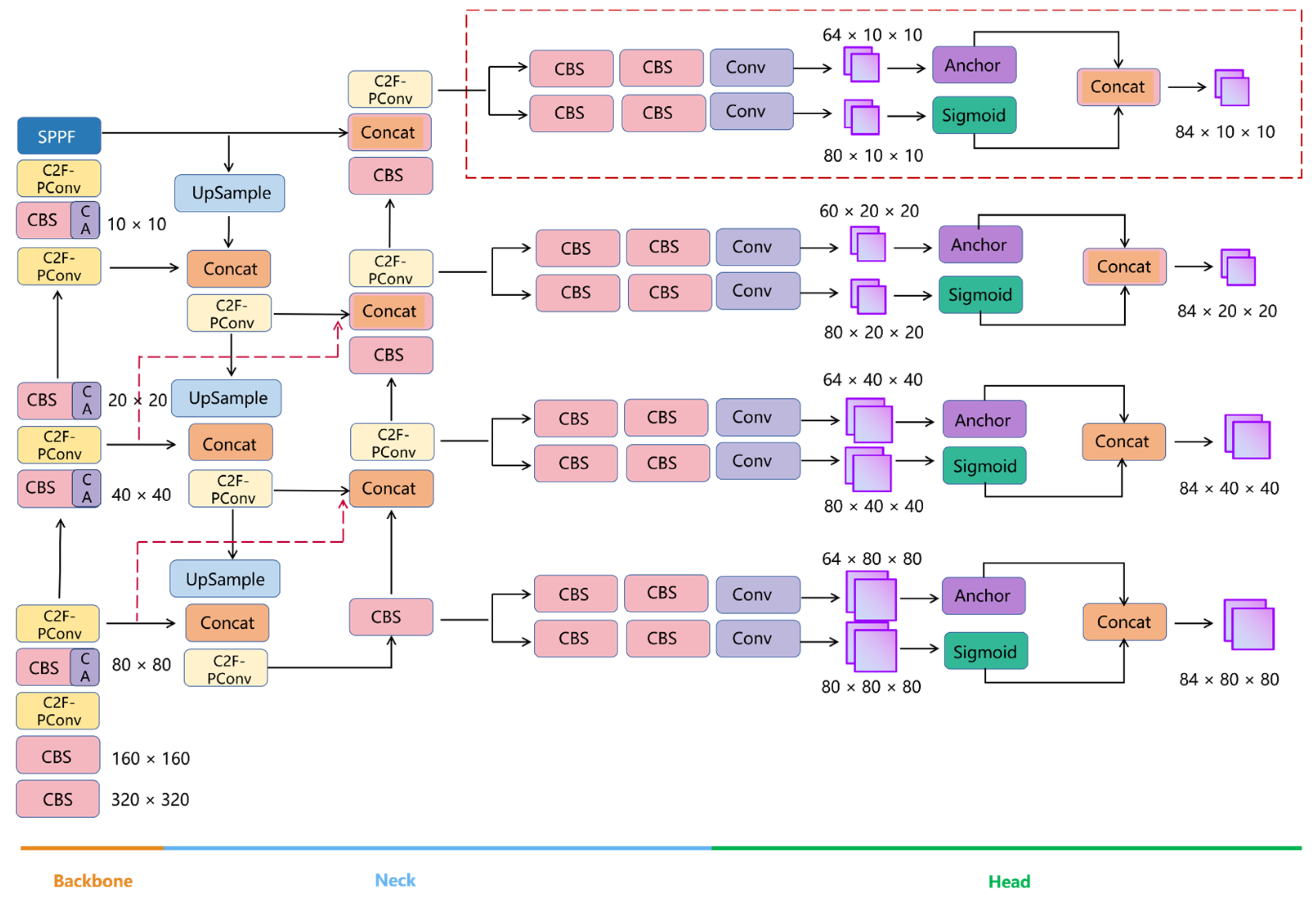
In this study, a CBS and C2F-Pconv were seamlessly integrated into the Backbone, yielding four distinct output routes, with the inclusion of a minimum detection box size of 10 × 10. In the Neck section, an additional C2F-Pconv was seamlessly incorporated into the left-side pathway, while the right-side pathway saw the strategic integration of a CBS, Concat, and C2F-Pconv. Furthermore, the Head section underwent enhancements with the addition of an extra 10 × 10 output. Within the right-side pathway, extending from the Backbone to the Neck, a fusion connection was introduced, adhering to the established BiFPN architecture. Initially, the fusion connection linked the third and fourth C2F layers from the Backbone to the right side; however, in this study, an innovative modification was implemented, connecting the second and third C2F layers instead. This alteration necessitated down-sampling to halve the height and width of the feature maps, facilitating seamless fusion with the right-side pathway. This design refinement significantly enhances the detection capabilities for small-scale targets [33]. The comprehensive enhancements and the detailed architecture of the upgraded Yolo8+ network model are vividly depicted in Figure 10.
5.4. Fusion Loss Function
By incorporating multiple loss functions, YOLOv8 leverages the strengths of different loss functions to mitigate the risk of overfitting, enhance model generalization, expedite convergence, boost training efficiency, and fortify the accuracy and robustness of object detection. Specifically, YOLOv8 utilizes VFL Loss for classification loss and combines CIoU Loss with DFL for regression loss. This amalgamation empowers YOLOv8 to excel in object detection challenges, yielding superior performance outcomes. The calculation formula of VFL Loss is shown in Equation (15), where q represents the intersection over union (IOU) between the predicted box and the ground truth box, and IOU represents the ratio of the intersection to the union of the predicted box and the ground truth box, while p represents the score or probability. When there is an intersection between the two boxes [34], q > 0, indicating a positive sample, and if there is no intersection, q = 0, indicating a negative sample.
The IOU loss function in YOLOv8 is the same as that in YOLOv5, and its calculation formula is shown in Equation (16), where IOU represents the intersection over union, b and represent the centroids of two rectangular boxes, p represents the Euclidean distance between the two rectangular boxes, c represents the diagonal distance of the enclosed regions of the two rectangular boxes, v is used to measure the consistency of the relative proportions of the two rectangular boxes, and a is the weighting coefficient [35].
For DFL, namely Distribution Focal Loss, in YOLOv8, the range of x1, y1, x2, y2 is defaulted to be between 0 and 15. This range is a hyperparameter related to the size of the targets on the feature map. As shown in the bottom-left part of Figure 9, the probability distribution of x1 ranges from 0 to 15 on the horizontal axis, consisting of 16 integers. x1 forms a discrete distribution, from which we can choose the integer with the highest probability as x1. For example, here, x1 takes the value of 8, which corresponds to the model directly predicting the left boundary of the detection box. However, this method is evidently inaccurate. In fact, we obtained the probability distribution of x1, from which we directly calculated the expected value. This expected value can replace the integer with the highest probability, specifically expressed by x×(x)dx.
In the equations, (x, y) and (, ), respectively, represent the coordinates of the anchor box and the target center point, while and denote the dimensions of the minimum enclosing box. IoU represents the intersection over union between the predicted box and the ground truth box, with parameters a and b typically set to 1.96 and 3.02, respectively. Furthermore, we introduced an outlier parameter to describe the quality of the anchor box, which is negatively correlated with the quality of the anchor box. The formula for computing the outlier degree is as follows.
The parameter in the range of the closed interval [0, +∞). represents the gradient increment in the monotonic aggregation coefficient, which is defined the same as LIoU, where * denotes dynamic adjustment based on the situation of each object detection during training. On the other hand, represents the sliding average of the momentum m; introducing allows for dynamically adjusting the maximum gradient gain according to the training progress. The calculation formula for momentum m is shown in Equation (18).
In this formula, where t represents the value of epoch and n represents the value of batch, the introduction of momentum m aims to allocate the small gradient gains in WIoU to low-quality anchor boxes after t rounds of training, thereby reducing the adverse impact of harmful gradients on model training.
The increased computational overhead of Wise-IOU (WIoU) primarily results from the computation of aggregation coefficients and the statistical calculation of mean IoU loss. Nevertheless, when compared to existing methods, WIoU exhibits improved efficiency due to its elimination of the need for aspect ratio computations. Consequently, upon integrating WIoU as the new loss function, a 30.2% reduction in training time was observed, accompanied by a 1.46% increase in accuracy under consistent experimental conditions.
6. Experimental Methods and Results
6.1. Network Training
The model training parameters were configured as follows: the maximum number of iterations was set to 500, utilizing stochastic gradient descent (SGD) [36] as the optimizer with a momentum value of 0.9. The learning rate adjustment strategy [37] employed cosine annealing decay, as outlined in Equation (19).
In the above formula, represents the initial learning rate, set to 0.08 in this experiment; represents the final learning rate, set to 0.000001 in this experiment [38]; nt represents the learning rate at the t-th iteration; and T represents the total number of iterations, set to 600 in this experiment.
6.2. Evaluation Metrics
In object recognition tasks, both the ground truth data and model predictions contain bounding boxes of objects along with their corresponding class information. Average precision (AP) is commonly used as a comparative metric, where a higher AP indicates closer proximity between the predicted results and the ground truth data. The computation of AP is based on precision () and recall (), defined as shown in Equations (20) and (21), respectively.
In the above formulas, , , and , respectively, represent the numbers of correctly identified, missed, and falsely identified samples. Average precision () refers to the integral of the precision–recall curve at different thresholds, indicating the comprehensive performance of precision under different recall rates. This is specifically shown in Equation (22).
Based on this approach, the average mean average precision (mAP) is calculated as the average of the average precisions for different classes. mAP@50 is derived by computing the mean average precision with an IOU threshold set to 0.5. For each individual class, the average precision (AP) is determined and then averaged across all classes to yield mAP@50. Moreover, mAP@50:95 represents the mean average precision calculated over IOU thresholds from 0.5 to 95%, incremented at 5% intervals, resulting in a total of 10 thresholds. By averaging the AP values at these various thresholds, mAP@50:95 serves as a comprehensive evaluation metric that offers a holistic assessment of the model’s object detection performance [39].
The changes in training set, validation set, P, and R are depicted in Figure 11. In the initial 100 epochs of training iterations, the loss rate of Yolov8+ rapidly decreases from 1 to 0.2. As the model surpasses 100 epochs of iterations, the loss rate gradually tends to plateau and exhibits a slow declining trend. P and R show a rapid fluctuating increase trend within the first 100 epochs of training iterations for Yolov8+, rising from 0.3 to 0.5. After over 100 epochs of iterations, the accuracy and recall stabilize at around 90.6% and 88.7%, respectively.
6.3. Ablation Experiment
A comparative analysis of the experimental results presented in Table 1 reveals the significant impact of various methods and combinations on the performance and efficiency of Yolov8+. The integration of the C2F-Pconv model into Yolov8 resulted in a marginal reduction in size by 1.51 MB and a corresponding decrease in detection time by 4.05 ms. However, a slight decline in the mAP metric was observed, indicating that the adoption of C2F-Pconv may lead to a trade-off between model complexity reduction and detection accuracy. On the other hand, Method (B) incorporated the CA attention module, which resulted in notable improvements in the mAP metric under both thresholds, with enhancements of 1.2% and 0.85%, despite the parameter size changes not being substantial. Moreover, the detection time remained within acceptable limits, highlighting the efficacy of the CA attention module in enhancing the overall model performance.
In Method (C), BiFPN was utilized for feature fusion. A substantial improvement in the mAP metric was observed compared to Yolov8s, with increases of 0.96% and 0.73% under both thresholds. Furthermore, there was a notable reduction in the detection time by 4.1%. This underscores the effectiveness of BiFPN in enhancing the model performance and expediting detection. On the other hand, Method (D) incorporated a fused loss function. Despite a significant reduction in the detection time by 7.1 ms, the mAP metrics were inferior to those of the original Yolov8, with decreases of 1.44% and 0.92% under the respective thresholds. This discrepancy may stem from the fused loss function’s potential limitations in certain scenarios, compromising detection accuracy while increasing model robustness. While utilizing individual modules in isolation can yield some performance enhancements, the optimal performance is not always achieved. This highlights the importance of identifying the optimal combination of methods, as a singular approach may not fully maximize the model’s capabilities.
6.4. Comparison with Other Mainstream Methods
Figure 12 illustrates the variation in mAP@50 across multiple training epochs. The Yolov5s model exhibits a relatively low mAP value from the initial epochs, and its final mAP value (85.1%) remains modest, indicating its limited performance. The mAP of the Yolov7 model also starts low during the early stages of training but maintains a steady increase throughout the entire training process, demonstrating a good optimization capability, with a final mAP value of 86.3%. The trend of mAP variation for the Yolov8 model is similar to that of Yolov7, but with a slightly higher overall level, reaching a final mAP value of 87.5%, indicating good optimization capability. As an improved version of Yolov8, the Yolov8+ model maintains the highest mAP value (89.1%) throughout the entire training process, fully demonstrating its effectiveness in optimization strategy and structural design, thereby significantly enhancing model performance.
Based on the results shown in Figure 13, which focuses on the evaluation metric mAP@50:95, the Yolov5s model exhibits relatively low mAP values in the initial epochs (0–50) [40]. However, as the number of epochs increases, the mAP value gradually improves and stabilizes around 66.8% at approximately epoch 200. In contrast, Yolov7 demonstrates higher mAP values from the initial stages and maintains relative stability throughout the entire training process, at around 67.2%. This indicates that Yolov7 possesses rapid convergence capabilities and strong robustness. The mAP values of Yolov8 are similar to those of Yolov7 in the initial stages, but as the epochs increase, its performance gradually surpasses that of Yolov7, stabilizing at around 68.4%. This suggests that Yolov8 exhibits good optimization potential during prolonged training. As an improved version of Yolov8, Yolov8+ consistently outperforms throughout the entire training process, achieving an mAP value of 71.1%. Particularly in the later epochs, its performance advantage becomes more significant, indicating the effectiveness of the improvements in the model structure and optimization strategy of Yolov8+.
6.5. Specific Detection Performance Chart
Based on the detection results depicted in Figure 14, this study analyzed outcomes following image enhancement. Colors including plastic film, soil, and maize shadows were removed from the original images, retaining only the green areas. This allowed us to observe the detection performance of the YOLOv8+ model in detecting early maize drought. In the figure, leaf areas marked with green boxes represent maize leaves suitable for growth, those marked with yellow boxes indicate maize leaves in a semi-drought state, while those marked with red boxes represent maize leaves in a drought state. The specific statistical quantities are shown in Table 2. These detection results are crucial for studying the growth status of maize plants in farmland and provide valuable monitoring tools for agricultural production.
7. Conclusions
In the context of large-scale mechanized and modern agriculture, traditional methods, such as ground inspection and soil moisture monitoring, face the challenges of a high workload and cost for the early drought detection of corn. Infrared imaging and hyperspectral imaging encounter challenges, including high costs, complex data processing and analysis, and significant weather influences. Additionally, detection standards vary across time and space. In recent years, with the rapid development of deep learning and precision agriculture, various advanced machine learning and deep learning models have been applied for the early drought detection of corn. These include digital image analysis techniques (color, texture, and plant morphology), deep convolutional neural networks (DCNNs), and customized convolutional neural networks. These models offer the advantages of automation, versatility, high accuracy, real-time capability, and tracking, meeting the needs of modern agricultural production. However, these models also face challenges. For instance, they require large amounts of high-quality data for algorithm training and involve high operational costs due to tuning performed by professionals and model optimization. Additionally, their usage conditions are limited, and practical applications in real scenarios can be challenging.
The experimental site for this study is located in the Hexi Corridor, Gansu Province, China. Our cultivated fields primarily feature maize seedlings, black plastic film, and drip irrigation belts as the target objects for detection. The drone-based object detection was performed at a height of 5 m, striking a balance between the detection field of view and accuracy. During the detection process, only the green color of maize seedlings is preserved, as other colors could potentially distort the detection results and hinder human observation of drought conditions. The climate here is arid, characterized by intense sunlight and frequent sandstorms. It is necessary to consider whether drones and deep learning models can still effectively detect drought under such conditions of intense sunlight. Of course, drone flights are suspended during sandstorms.
The study introduces the Yolov8+ model, incorporating unmanned aerial vehicle (UAV) images, to develop an automated and cost-effective model that exhibits an outstanding performance in practical applications. In the Backbone section, the utilization of the C2F-Conv module reduces the model’s floating-point operations and computational complexity, thereby decreasing the model’s parameter count and computational costs, leading to a reduction in deployment expenses. Additionally, the incorporation of the Coordinate Attention (CA) mechanism enhances the model’s suitability for UAV target monitoring by effectively capturing minute feature information in images and addressing the sparsity of feature information across different drought categories. The Neck section of the Yolov8+ model adopts BiFPN fusion architecture and introduces a spatial attention mechanism to address insufficient long-distance information transmission in target detection, enhancing the model’s recognition capabilities for small and obstructed targets, and displaying a superior performance in practical applications. Furthermore, the Head section of the model introduces a 10 × 10 output and improves the loss function, resulting in a 1.46% increase in accuracy, a 30.2% reduction in training time, and enhanced model robustness.
The improved YOLOv8+ model demonstrates significant advancements in model structure and optimization strategies, achieving mAP@50 and mAP@50:95 scores of 89.16% and 71.14%, respectively. It boasts a high UAV image detection speed of 24.63 ms and a model size of 13.76 MB. Our ongoing future work involves accurately integrating the drought conditions detected from UAV imagery with the farm irrigation system. Additionally, we will continue to refine the model to achieve drought detection at each growth stage of maize. We are honored to have received support from the Key Science and Technology Development Fund of China for our project, titled “Key Technology Research and Development for High Water Efficiency Precision Agriculture Production in Hexi Oasis Irrigation Area”.
Farmers and agricultural professionals do not need to invest a significant amount of time and money in training, nor do they need to possess advanced technical expertise or rely on expensive specialized equipment. In the current scenario of escalating global climate change, this model effectively addresses irrational irrigation practices in drought-affected regions, leading to water resource conservation. It resolves the challenge of traditional manual surveillance methods being insufficient for efficiently monitoring large agricultural areas. Additionally, it is applicable for monitoring seedling growth, assessing planting environments, and predicting yields. By leveraging UAV images and deep learning technologies, this model paves the way for sustainable and modern agricultural production, significantly advancing the field.
Author Contributions
Conceptualization, S.N.; methodology, S.N.; validation, S.N. and W.Z.; formal analysis, W.Z.; investigation, W.Z.; data curation, W.Z.; writing—original draft, Z.N.; supervision, G.L.; project administration, Z.N. and G.L.; funding acquisition, Z.N. and G.L. All authors have read and agreed to the published version of the manuscript.
Funding
This project was supported by the Youth Tutor Support Fund of Gansu Agricultural University (GAU-QDFC-2022-19), the Industrial Support Program Project of Gansu Provincial Department of Education (2022CYZC-41), and the Leading Talent Program of Gansu Province (GSBJLJ-2023-09).
Data Availability Statement
Data can be requested from the corresponding authors and the first author via email.
Conflicts of Interest
The authors declare no conflicts of interest.
References
- Guo, E.; Liu, X.; Zhang, J.; Wang, Y.; Wang, C.; Wang, R.; Li, D. Assessing spatiotemporal variation of drought and its impact on maize yield in Northeast China. J. Hydrol. 2017, 553, 231–247. [Google Scholar] [CrossRef]
- Herrero-Huerta, M.; Gonzalez-Aguilera, D.; Yang, Y. Structural Component Phenotypic Traits from Individual Maize Skeletonization by UAS-Based Structure-from-Motion Photogrammetry. Drones 2023, 7, 108. [Google Scholar] [CrossRef]
- Liu, Y.; Subhash, C.; Yan, J.; Song, C.; Zhao, J.; Li, J. Maize leaf temperature responses to drought: Thermal imaging and quantitative trait loci (QTL) mapping. Environ. Exp. Bot. 2011, 71, 158–165. [Google Scholar] [CrossRef]
- Mertens, S.; Verbraeken, L.; Sprenger, H.; Demuynck, K.; Maleux, K.; Cannoot, B.; De Block, J.; Maere, S.; Nelissen1, H.; Bonaventure, G.; et al. Proximal hyperspectral imaging detects diurnal and drought-induced changes in maize physiology. Front. Plant Sci. 2021, 12, 640914. [Google Scholar] [CrossRef] [PubMed]
- Brewer, K.; Clulow, A.; Sibanda, M.; Gokool, S.; Odindi, J.; Mutanga, O.; Naiken, V.; Chimonyo, V.G.P.; Mabhaudhi, T. Estimation of maize foliar temperature and stomatal conductance as indicators of water stress based on optical and thermal imagery acquired using an unmanned aerial vehicle (UAV) platform. Drones 2022, 6, 169. [Google Scholar] [CrossRef]
- Pradawet, C.; Khongdee, N.; Pansak, W.; Spreer, W.; Hilger, T.; Cadisch, G. Thermal imaging for assessment of maize water stress and yield prediction under drought conditions. J. Agron. Crop Sci. 2023, 209, 56–70. [Google Scholar] [CrossRef]
- Praprotnik, E.; Vončina, A.; Žigon, P.; Knapič, M.; Susič, N.; Širca, S.; Vodnik, D.; Lenarčič, D.; Lapajne, J.; Žibrat, U.; et al. Early Detection of Wireworm (Coleoptera: Elateridae) Infestation and Drought Stress in Maize Using Hyperspectral Imaging. Agronomy 2023, 13, 178. [Google Scholar] [CrossRef]
- Jiang, B.; Wang, P.; Zhuang, S.; Li, M.; Li, Z.; Gong, Z. Detection of maize drought based on texture and morphological features. Comput. Electron. Agric. 2018, 151, 50–60. [Google Scholar] [CrossRef]
- Zhuang, S.; Wang, P.; Jiang, B.; Li, M.; Gong, Z. Early detection of water stress in maize based on digital images. Comput. Electron. Agric. 2017, 140, 461–468. [Google Scholar] [CrossRef]
- An, J.; Li, W.; Li, M.; Cui, S.; Yue, H. Identification and classification of maize drought stress using deep convolutional neural network. Symmetry 2019, 11, 256. [Google Scholar] [CrossRef]
- Goyal, P.; Sharda, R.; Saini, M.; Siag, M. A deep learning approach for early detection of drought stress in maize using proximal scale digital images. Neural Comput. Appl. 2024, 36, 1899–1913. [Google Scholar] [CrossRef]
- Fu, X.; Wei, G.; Yuan, X.; Liang, Y.; Bo, Y. Efficient YOLOv7-Drone: An Enhanced Object Detection Approach for Drone Aerial Imagery. Drones 2023, 7, 616. [Google Scholar] [CrossRef]
- Pu, H.; Chen, X.; Yang, Y.; Tang, R.; Luo, J.; Wang, Y.; Mu, J. Tassel-YOLO: A new high-precision and real-time method for maize tassel detection and counting based on UAV aerial images. Drones 2023, 7, 492. [Google Scholar] [CrossRef]
- Wang, J.; Zhang, H.; Liu, Y.; Zhang, H.; Zheng, D. Tree-Level Chinese Fir Detection Using UAV RGB Imagery and YOLO-DCAM. Remote Sens. 2024, 16, 335. [Google Scholar] [CrossRef]
- Tian, Y.; Zhang, K.; Hu, X.; Lu, Y. Crop type recognition of VGI road-side images via hierarchy structure based on semantic segmentation model Deeplabv3+. Displays 2024, 81, 102574. [Google Scholar] [CrossRef]
- Zhao, H.; Wan, F.; Lei, G.; Xiong, Y.; Xu, L.; Xu, C.; Zhou, W. LSD-YOLOv5: A Steel Strip Surface Defect Detection Algorithm Based on Lightweight Network and Enhanced Feature Fusion Mode. Sensors 2023, 23, 6558. [Google Scholar] [CrossRef] [PubMed]
- Huang, Y.; Zhuo, Q.; Fu, J.; Liu, A. Research on evaluation method of underwater image quality and performance of underwater structure defect detection model. Eng. Struct. 2024, 306, 117797. [Google Scholar] [CrossRef]
- Tahir, N.U.A.; Long, Z.; Zhang, Z.; Asim, M.; ELAffendi, M. PVswin-YOLOv8s: UAV-Based Pedestrian and Vehicle Detection for Traffic Management in Smart Cities Using Improved YOLOv8. Drones 2024, 8, 84. [Google Scholar] [CrossRef]
- Wang, X.; Han, J.; Xiang, H.; Wang, B.; Wang, G.; Shi, H.; Chen, L.; Wang, Q. A Lightweight Traffic Lights Detection and Recognition Method for Mobile Platform. Drones 2023, 7, 293. [Google Scholar] [CrossRef]
- Singhania, D.; Rahaman, R.; Yao, A. C2F-TCN: A framework for semi-and fully-supervised temporal action segmentation. IEEE Trans. Pattern Anal. Mach. Intell. 2023, 45, 11484–11501. [Google Scholar] [CrossRef]
- Jeng, K.-Y.; Liu, Y.-C.; Liu, Z.Y.; Wang, J.-W.; Chang, Y.-L.; Su, H.-T.; Hsu, W. Gdn: A coarse-to-fine (c2f) representation for end-to-end 6-dof grasp detection. In Proceedings of the 4th Conference on Robot Learning (PMLR), Cambridge MA, USA, 16–18 November 2021. [Google Scholar]
- Yu, X.; Xu, L.; Li, J.; Ji, X. MagConv: Mask-guided convolution for image inpainting. IEEE Trans. Image Process. 2023, 32, 4716–4727. [Google Scholar] [CrossRef] [PubMed]
- Zeng, W.; Li, H.; Hu, G.; Liang, D. Lightweight dense-scale network (LDSNet) for corn leaf disease identification. Comput. Electron. Agric. 2022, 197, 106943. [Google Scholar] [CrossRef]
- Wang, W.; Han, B.; Guo, Y.; Luo, X.; Yuan, M. Fault-tolerant platoon control of autonomous vehicles based on event-triggered control strategy. IEEE Access 2020, 8, 25122–25134. [Google Scholar] [CrossRef]
- Hou, Q.; Zhou, D.; Feng, J. Coordinate attention for efficient mobile network design. In Proceedings of the IEEE/CVF Conference on Computer Vision and Pattern Recognition, Nashville, TN, USA, 20–25 June 2021. [Google Scholar]
- Zhao, L.; Zhu, M. MS-YOLOv7: YOLOv7 based on multi-scale for object detection on UAV aerial photography. Drones 2023, 7, 188. [Google Scholar] [CrossRef]
- Raturi, A.; Jennifer, J.; Thompson, V.A.; Chase, C.A.; Davis, B.W.; Myers, R.; Poncet, A.; Ramos-Giraldo, P.; Reberg-Horton, C.; Rejesus, R.; et al. Cultivating trust in technology-mediated sustainable agricultural research. Agron. J. 2022, 114, 2669–2680. [Google Scholar] [CrossRef]
- Seth, A.; James, A.; Kuantama, E.; Mukhopadhyay, S.; Han, R. Drone High-Rise Aerial Delivery with Vertical Grid Screening. Drones 2023, 7, 300. [Google Scholar] [CrossRef]
- Chen, J.; Mai, H.S.; Luo, L.; Chen, X.; Wu, K. Effective feature fusion network in BIFPN for small object detection. In Proceedings of the 2021 IEEE International Conference on Image Processing (ICIP), Anchorage, AK, USA, 19–22 September 2021; IEEE: Piscataway, NJ, USA, 2021. [Google Scholar]
- Zhu, X.; Cheng, D.; Zhang, Z.; Lin, S.; Dai, J. An empirical study of spatial attention mechanisms in deep networks. In Proceedings of the IEEE/CVF International Conference on Computer Vision, Seoul, Republic of Korea, 27 October–2 November 2019. [Google Scholar]
- Angelis, G.-F.; Chorozoglou, D.; Papadopoulos, S.; Drosou, A.; Giakoumis, D.; Tzovaras, D. AI-enabled Underground Water Pipe non-destructive Inspection. Multimed. Tools Appl. 2023, 83, 18309–18332. [Google Scholar] [CrossRef]
- Saeed, Z.; Yousaf, M.H.; Ahmed, R.; Velastin, S.A.; Viriri, S. On-board small-scale object detection for unmanned aerial vehicles (UAVs). Drones 2023, 7, 310. [Google Scholar] [CrossRef]
- Hussain, M. YOLO-v1 to YOLO-v8, the rise of YOLO and its complementary nature toward digital manufacturing and industrial defect detection. Machines 2023, 11, 677. [Google Scholar] [CrossRef]
- Talaat, F.M.; Hanaa, Z. An improved fire detection approach based on YOLO-v8 for smart cities. Neural Comput. Appl. 2023, 35, 20939–20954. [Google Scholar] [CrossRef]
- Chang, Y.; Li, D.; Gao, Y.; Su, Y.; Jia, X. An improved YOLO model for UAV fuzzy small target image detection. Appl. Sci. 2023, 13, 5409. [Google Scholar] [CrossRef]
- Wang, J.; Gauri, J. Cooperative SGD: A unified framework for the design and analysis of local-update SGD algorithms. J. Mach. Learn. Res. 2021, 22, 1–50. [Google Scholar]
- Boukabou, I.; Kaabouch, N. Electric and magnetic fields analysis of the safety distance for UAV inspection around extra-high voltage transmission lines. Drones 2024, 8, 47. [Google Scholar] [CrossRef]
- Shi, Y.; Li, X.; Wang, G.; Jin, X. Research on the Recognition and Classification of Recyclable Garbage in a Complex Environment Based on Improved YOLOv8s. In Proceedings of the 2023 5th International Conference on Control and Robotics (ICCR), Tokyo, Japan, 23–25 November 2023; IEEE: Piscataway, NJ, USA, 2023. [Google Scholar]
- Liu, Y.; Huang, X.; Liu, D. Weather-Domain Transfer-Based Attention YOLO for Multi-Domain Insulator Defect Detection and Classification in UAV Images. Entropy 2024, 26, 136. [Google Scholar] [CrossRef]
- Wei, B.; Barczyk, M. Experimental Evaluation of Computer Vision and Machine Learning-Based UAV Detection and Ranging. Drones 2021, 5, 37. [Google Scholar] [CrossRef]
Figure 1.
The schematic diagram of the research work in this paper. (a) A800 computing power server, (b) Unmanned aerial vehicle (UAV). (c) Pilot field of oasis irrigation area in Hexi Corridor. (d) Early-stage images of corn at a height of 5 m (UAV). (e) Post-inspection situation chart (green box indicates suitable condition, yellow box indicates semi-drought condition, and red box indicates drought condition).

Figure 2.
Sample collection of data images. (a) Data collection site; (b) multispectral images; (c) images taken from a height of 5 m; (d) super-green factor transformed images; (e) binary transformed images; (f) Sobel operator edge extraction images.
Figure 2.
Sample collection of data images. (a) Data collection site; (b) multispectral images; (c) images taken from a height of 5 m; (d) super-green factor transformed images; (e) binary transformed images; (f) Sobel operator edge extraction images.

Figure 3.
Three different categories of dataset images. (a) Drought category data sample images; (b) semi-arid category data sample images; (c) images of optimal category data samples.
Figure 3.
Three different categories of dataset images. (a) Drought category data sample images; (b) semi-arid category data sample images; (c) images of optimal category data samples.

Figure 4.
Sample YOLOv8 network architecture diagram. Notes: “Conv” represents the convolution module composed of Conv2d, Batch Normalization, and SiLU activation function. “C2F” denotes the cross-connection and feature fusion of feature maps. “Concat” signifies dimension concatenation. “Upsample” refers to upsampling. “SPPF” indicates spatial pyramid pooling structure. “Anchor” is utilized for generating target detection boxes. “Sigmoid” is an activation function that transforms the confidence of each class into a probability between 0 and 1.

Figure 5.
Diagram of the C2F module and Anchor module. Notes: In this structure, “Split” indicates channel division. “BottleNeck” signifies enhancing the non-linearity of the network to better capture and represent feature information in images. The function of “SoftMax” is to normalize the 16 feature channels. “Conv” denotes the convolution module. “Gap” represents global average pooling. “Grid” refers to the grid structure of the network.

Figure 6.
C2F-Pconv module schematic diagram.

Figure 7.
The structural principle of the coordinate attention mechanism. Notes: The notation “X avg pool” denotes horizontal average pooling, while “Y avg pool” refers to vertical average pooling. “Batch Norm” indicates the batch normalization operation, which is utilized to improve the convergence speed of the model. The variables H, W, and C represent the height, width, and feature channels of the feature map, respectively.

Figure 8.
Illustration of the BiFPN structure. Notes: In the backbone section, as each additional route of feature maps is outputted, the height and width of the feature maps decrease by half.
Figure 8.
Illustration of the BiFPN structure. Notes: In the backbone section, as each additional route of feature maps is outputted, the height and width of the feature maps decrease by half.

Figure 9.
Calculation process of the detection boxes.

Figure 10.
The network architecture diagram of the improved Yolov8+.

Figure 11.
Test, train, precision, and recall training variation curves. Notes: The training consists of 500 epochs.
Figure 11.
Test, train, precision, and recall training variation curves. Notes: The training consists of 500 epochs.

Figure 12.
The precision variation curve of the mAP@50 metric across different algorithms. Notes: The four algorithms are Yolov8+, Yolov8, Yolov7, and Yolov5s.
Figure 12.
The precision variation curve of the mAP@50 metric across different algorithms. Notes: The four algorithms are Yolov8+, Yolov8, Yolov7, and Yolov5s.

Figure 13.
The precision variation curve of the mAP@50:95 metric across different algorithms. Notes: The four algorithms are Yolov8+, Yolov8, Yolov7, and Yolov5s.
Figure 13.
The precision variation curve of the mAP@50:95 metric across different algorithms. Notes: The four algorithms are Yolov8+, Yolov8, Yolov7, and Yolov5s.

Figure 14.
The specific detection results of the YOLOv8+ model. Notes: The red detection box represents leaves under drought conditions, the yellow detection box represents leaves under semi-drought conditions, and the green detection box represents leaves under suitable conditions.
Figure 14.
The specific detection results of the YOLOv8+ model. Notes: The red detection box represents leaves under drought conditions, the yellow detection box represents leaves under semi-drought conditions, and the green detection box represents leaves under suitable conditions.


Table 1.
Comparison of ablation experiments with different modules. Notes: A series of ablation experiments were conducted to investigate different improvement methods, including the C2F-Pconv module, CA attention mechanism module, BiFPN feature fusion structure, and fused loss function. “—” indicates that the module has not been added, while “√” indicates that the module has been added.
| Method | C2F-Pconv | CA Model | BiFPN Fusion | Loss Function | Params/MB | mAP@50/% | mAP@50:95/% | Detection Time/ms |
|---|---|---|---|---|---|---|---|---|
| Yolov8 | — | — | — | — | 20.13 | 85.26 | 67.84 | 34.63 |
| (A) | √ | — | — | — | 18.62 | 85.02 | 67.36 | 30.28 |
| (B) | — | √ | — | — | 19.21 | 86.46 | 68.69 | 31.18 |
| (C) | — | — | √ | — | 18.93 | 87.91 | 68.53 | 30.53 |
| (D) | — | — | — | √ | 19.30 | 86.7 | 66.92 | 27.53 |
| (E) | √ | √ | — | — | 18.38 | 86.86 | 68.20 | 27.82 |
| (F) | √ | — | √ | — | 18.53 | 87.21 | 68.51 | 26.94 |
| (G) | √ | — | — | √ | 17.26 | 87.13 | 68.26 | 26.17 |
| (H) | — | √ | √ | — | 17.83 | 87.59 | 69.13 | 26.45 |
| (I) | — | √ | — | √ | 16.58 | 87.27 | 68.90 | 26.15 |
| (J) | — | — | √ | √ | 16.64 | 87.53 | 68.43 | 25.93 |
| (K) | √ | √ | √ | — | 15.83 | 88.21 | 69.32 | 25.76 |
| (L) | √ | — | √ | √ | 15.47 | 88.62 | 69.64 | 25.49 |
| (M) | — | √ | √ | √ | 14.42 | 88.79 | 70.84 | 25.08 |
| (N) | √ | √ | √ | √ | 13.76 | 89.16 | 71.14 | 24.63 |
Table 2.
Statistics of maize leaf quantities under three different states: drought, semi-drought, and optimal. Notes: The unit in the table is in numbers.
Table 2.
Statistics of maize leaf quantities under three different states: drought, semi-drought, and optimal. Notes: The unit in the table is in numbers.
| Drought | Semi-Drought | Optimal | |
|---|---|---|---|
| The first line | 4 | 50 | 45 |
| The second line | 4 | 37 | 77 |
| The third line | 4 | 51 | 58 |
| The fourth line | 0 | 19 | 88 |
Disclaimer/Publisher’s Note: The statements, opinions and data contained in all publications are solely those of the individual author(s) and contributor(s) and not of MDPI and/or the editor(s). MDPI and/or the editor(s) disclaim responsibility for any injury to people or property resulting from any ideas, methods, instructions or products referred to in the content. |
© 2024 by the authors. Licensee MDPI, Basel, Switzerland. This article is an open access article distributed under the terms and conditions of the Creative Commons Attribution (CC BY) license (https://creativecommons.org/licenses/by/4.0/).
Share and Cite
MDPI and ACS Style
Niu, S.; Nie, Z.; Li, G.; Zhu, W. Early Drought Detection in Maize Using UAV Images and YOLOv8+. Drones 2024, 8, 170. https://doi.org/10.3390/drones8050170
AMA Style
Niu S, Nie Z, Li G, Zhu W. Early Drought Detection in Maize Using UAV Images and YOLOv8+. Drones. 2024; 8(5):170. https://doi.org/10.3390/drones8050170
Chicago/Turabian StyleNiu, Shanwei, Zhigang Nie, Guang Li, and Wenyu Zhu. 2024. "Early Drought Detection in Maize Using UAV Images and YOLOv8+" Drones 8, no. 5: 170. https://doi.org/10.3390/drones8050170