
Enhancing UAV Aerial Docking: A Hybrid Approach Combining Offline and Online Reinforcement Learning


The School of Mechatronical Engineering, Beijing Institute of Technology, Beijing 100081, China
*
Author to whom correspondence should be addressed.
Drones 2024, 8(5), 168; https://doi.org/10.3390/drones8050168
Submission received: 5 March 2024
/
Revised: 12 April 2024
/
Accepted: 22 April 2024
/
Published: 24 April 2024
Abstract
:In our study, we explore the task of performing docking maneuvers between two unmanned aerial vehicles (UAVs) using a combination of offline and online reinforcement learning (RL) methods. This task requires a UAV to accomplish external docking while maintaining stable flight control, representing two distinct types of objectives at the task execution level. Direct online RL training could lead to catastrophic forgetting, resulting in training failure. To overcome these challenges, we design a rule-based expert controller and accumulate an extensive dataset. Based on this, we concurrently design a series of rewards and train a guiding policy through offline RL. Then, we conduct comparative verification on different RL methods, ultimately selecting online RL to fine-tune the model trained offline. This strategy effectively combines the efficiency of offline RL with the exploratory capabilities of online RL. Our approach improves the success rate of the UAV’s aerial docking task, increasing it from 40% under the expert policy to 95%.
1. Introduction
In recent years, with the increasing prevalence of autonomous robots, UAVs in the aviation sector have garnered a great deal of attention. UAVs have demonstrated immense applicability in various domains, such as cinematography, visual inspection, communications, and networking [1,2,3]. However, their size, motors, and other components limit their effective payload capacity. When multiple UAVs are integrated into a cohesive system known as a multiple aerial vehicle assembly (MAVA), they can achieve higher load-bearing capabilities and perform more complex tasks [4,5,6,7,8,9]. However, this assembled structure compromises the system’s maneuverability, particularly in confined spaces, posing greater challenges to the completion of more specific tasks. Therefore, the design of effective aerial vehicle docking and separation control mechanisms has become crucial. TRADY [10] is engineered as an aerial unit with the capability for autonomous assembly and disassembly in flight. However, the execution of this task necessitates a specialized UAV equipped with a magnetic docking mechanism. This prerequisite presents a considerable challenge when attempting to modify existing MAVA platforms. We implement a modification to the F450 subunits of the MAVA platform, realizing a novel docking mechanism.
RL has found extensive applications in the domain of quadrotors [11,12]. It is often observed that RL may not match the accuracy of traditional optimal control methods in control-oriented tasks. However, it tends to demonstrate superior robustness and effectiveness in manipulation tasks [13,14]. The proximal policy optimization (PPO) [15] algorithm has also demonstrated some advantages [16,17]. The advantage of RL lies not in its superior optimization of the objective, but in its optimization of a better objective. In optimal control, the task is typically decomposed into planning and control when accomplishing the objective. This decomposition limits the range of behaviors that the controller can express, leading to poor control performance when facing unmodeled effects. In contrast, RL can directly optimize task-level objectives and use domain randomization to cope with model uncertainty, thereby discovering more robust control responses. However, RL training is not straightforward, as it usually requires extensive tuning of the reward function and the simulation environment, and it may not guarantee successful learning [18].
Most existing RL algorithms start from scratch to collect data online each time they learn a new strategy. This quickly becomes impractical in fields such as robotics, where the cost of physical data collection is high. Just as powerful models in computer vision and natural language processing are typically pre-trained on large general datasets and then fine-tuned on specific task data, practical instances of RL for real-world robotic problems need to be able to effectively integrate a large amount of prior data into the learning process, while still collecting additional data online for the task at hand. Doing so effectively will make the online data collection process more practical, while still allowing robots to operate in the real world to continue improving their behavior.
Previous studies have indicated that RL is vulnerable to catastrophic forgetting during training, mainly due to the presence of multiple and conflicting learning objectives [19]. This issue also arises in the docking process: first, learning how to control the quadrotors’ movement; second, learning how to avoid collision and maintain stability during the docking process; the third objective involves mastering the ability to maintain a stable hover for the pair of quadrotors post-docking. The primary items in accomplishing successful training are bifurcated into two aspects: the formulation of a suitable reward function tailored for the docking procedure, and the circumvention of catastrophic forgetting that arises due to the presence of multiple objectives.
Inverse reinforcement learning (IRL) emerges as a viable technique when the reward function is elusive to define [20,21,22]. It possesses the capability to autonomously discern a reward function from expert demonstrations, a characteristic exemplified by generative adversarial imitation learning (GAIL) [23]. Certain algorithms, such as adversarial motion prior (AMP) [24,25,26], streamline the reward function design by assimilating expert policy data. However, these algorithms are typically plagued by intricate parameter tuning, sluggish convergence, and an inability to mitigate the catastrophic forgetting issue.
Behavioral cloning (BC) [27] is a methodology that can encapsulate an expert policy into a neural network [28]. However, it generally necessitates a substantial volume of data, and its performance is upper-bounded by the expertise level [29]. In scenarios of data paucity, BC is susceptible to a pronounced out-of-distribution (OOD) problem [30]. BC exhibits efficacy when the expert policy is optimal. Conversely, in the presence of a suboptimal expert policy, offline RL can enhance the expert policy, provided there is an abundance of data [31,32,33,34].
The twin delayed deep deterministic policy gradient with behavior cloning (TD3BC) algorithm [33] can mitigate the OOD problem in Offline RL to some extent. The TD3BC algorithm introduces a regularization term in the calculation of policy gradients, making the learning policy as close as possible to the behavior policy. This can reduce the exploration of the policy in the OOD region, thereby reducing the overestimation problem caused by it. Implicit Q-learning (IQL) [35], as an offline RL algorithm, primarily refrains from evaluating the Q-value of the latest policy under unseen actions. Instead, it implicitly estimates the policy improvement step by considering the Q-value of the optimal action under a state as a random variable determined by the action. This approach alleviates the OOD problem in offline RL to a certain extent.
Since offline RL can only perform limited exploration [35,36,37,38,39,40,41,42], the policy learned by offline RL is generally suboptimal as well, but online RL can discover a better policy. So the integration of online and offline RL offers several advantages. It allows for the efficient use of previously collected data (offline learning), while still enabling the model to adapt to new information as it interacts with the environment (online learning). This hybrid approach can lead to more robust and adaptable models. Specifically, offline learning can provide a solid foundation of knowledge, reducing the amount of exploration needed during online learning. Meanwhile, online learning allows the model to continually refine its strategies based on new experiences, leading to ongoing performance improvements. This combination can result in more effective learning, particularly in complex, dynamic environments where the ability to leverage both historical data and new experiences is crucial. This paper tackles the issue of catastrophic forgetting in online RL by utilizing a guidance policy derived from offline RL. As a result, this methodology markedly improves the success rate of docking tasks.
Our contributions are summarized as follows:
- We developed an expert strategy scheme that combines hybrid force/position control to solve the docking problem during the interaction process of two quadrotors.
- For aerial docking tasks, we designed effective rewards for RL to support strategy training.
- We efficiently combined offline learning and online learning strategies in RL, effectively increasing the success rate of the entire training task to 95%.
The organization of this paper is as follows: Section 2 delves into the problem definition, providing a comprehensive description of the quadrotor dynamics, the thrust-omega controller, and the descriptions of RL. Section 3 meticulously outlines the method used, organized around the Rule-Based Expert Policy, Offline-to-Online RL, and the reward function. In Section 4, we test our distinctive approach to the docking task. Here, we conduct experiments with a variety of online and offline RL strategies and delve into an exploration of a fusion method that integrates offline-to-online methods. Finally, Section 5 wraps up the paper with a conclusion and sketches out potential directions for future work.
2. Problem Definition
2.1. Quadrotor Dynamics
The dynamics of each quadrotor are characterized by the state , encompassing the position in the world frame, velocity also in the world frame, rotation matrix from the body to the world frame, and angular velocity in the body frame. The dynamics of the quadrotor are delineated as follows:
where g denotes the gravitational acceleration, m represents the mass of the quadrotor, , corresponds to the thrust in the body frame, signifies the contact force with environment in the world frame, is the inertia matrix of the quadrotor, and is the total torque in the body frame, is a skew-symmetric matrix associated with rotated to the world frame. In (2), is calculated as follows:
where is the thrust of a single propeller in the body frame, is the position of the propeller in the body frame, and is the torque-to-thrust coefficient.
We employ RaiSim v1.1.01 [43] to develop a quadrotor simulator, which accurately simulates collisions and contact scenarios between two quadrotors.
2.2. Thrust-Omega Controller
The input of the environment is normalized accelerations along the z-axis in the world coordinate system, coupled with angular velocities in the body frame for each quadrotor. The policy (from the expert or RL) outputs normalized motor thrust and angular velocity values through the following thrust-omega controller, which applies forces to the four rotors of a quadrotor in the RaiSim environment via an open API, thereby driving the UAV’s motion.
Normalized motor thrust is computed as follows:
where , g is the gravitational acceleration. is the target angular acceleration of the quadrotor. And M is the control efficiency matrix [44] defined as follows:
where l is the distance between the center of mass and the motor, is the torque-to-thrust coefficient, and is the maximum thrust of the motor. could be computed by:
where . and are the proportional and integral gains.
2.3. Reinforcement Learning
Reinforcement learning is a field of machine learning that emphasizes how to act based on the environment to achieve maximum expected benefit. It is the third basic machine learning method besides supervised learning and unsupervised learning. Unlike supervised learning, RL does not require labeled input-output pairs, nor does it need to precisely correct non-optimal solutions. Its focus is on finding a balance between exploration (of unknown areas) and exploitation (of existing knowledge). The inspiration for RL comes from behavioral theories in psychology, how organisms gradually form expectations of stimuli and habitual behaviors that can obtain maximum benefits under the stimuli of rewards or punishments given by the environment. This method is universal, so it has been studied in many fields, such as education, marketing, robotics, gaming, autonomous driving, natural language processing, internet of things security, recommendation systems, finance, and energy management [45,46].
RL can be categorized in various ways, including model-based versus model-free, value-based versus policy-based, on-policy versus off-policy, and so on. Methods for solving RL problems that use models and planning are called model-based methods, as opposed to simpler model-free methods that are explicitly trial-and-error learners—viewed as almost the opposite of planning [47]. Model-free approaches require more data and diverse experience to learn the task than model-based methods, but model-free approaches often produce better performance than model-based methods [48]. Value-based methods aim to find the value of each state or state-action pair and select the optimal action based on these values. This could result in a slow learning process. Policy-based algorithm directly optimizes the policy that determines the agent’s behavior [49]. It could solve the continued action space during the training process. On-policy and off-policy refer to two different training methodologies, distinguished by whether the behavior policy and the target policy are the same [50]. On-policy methods follow and improve on the same policy throughout the learning process, allowing them to converge to the optimal policy in deterministic environments. However, a major drawback of on-policy methods is their inability to effectively utilize old or offline experiences, as they require collecting new experiences under the current policy. Off-policy methods can learn from one policy while improving upon another policy simultaneously. This enables them to effectively utilize old or offline experiences. Off-policy methods may require more complex learning algorithms since they need to handle experiences from different policies.
Both PPO and TD3BC belong to the category of model-free algorithms. They offer some advantages in performance over model-based algorithms. Q-learning and Deep Q-Networks (DQN) are value-based methods. These methods may struggle with large-scale or continuous action spaces, as they need to evaluate the value function for each action. On the other hand, PPO has recently gained popularity for its robustness and simplicity. And it is well-suited for RL problems with continuous state and action spaces where interacting with the environment is not considered expensive [18,51]. However, as an on-policy algorithm, PPO does not utilize training data efficiently and can lead to phase forgetting in the face of complex docking tasks at hand, making the final model difficult to converge. TD3BC, as an off-policy algorithm, uses experience replay to alleviate sample correlation and employs a dual Q-value network to reduce overestimation errors, thereby improving sample efficiency. It also mitigates phase forgetting through data replay. However, considering that offline algorithms may lack environmental exploration capabilities, we propose a combination of offline and online methods to accomplish our current docking task.
RL can be formulated as a Markov Decision Process (MDP). An MDP is defined by a tuple (, , , r, ) [47], where is the state space, is the action space, is the transition probability, r is the reward function, and is the discount factor. The goal of RL is to find a policy that maximizes the expected return , where is a trajectory sampled from the policy . d denotes the done flag, which indicates whether the episode is terminated.
3. Method
As shown in Figure 1, the docking apparatus comprises two quadrotors, each equipped with a docking device. One quadrotor features a cylindrical recess, while the other is fitted with a conical tip designed to fit precisely within the recess. This design was meticulously crafted using SolidWorks. For the docking procedure, the recess is attached to quadrotor A and the tip to quadrotor B. The docking task is deemed successful once the tip is fully inserted into the cylindrical recess, and the controller is able to maintain stable flight of the now unified quadrotors.
3.1. Rule-Based Expert Policy
The collection of expert data is a pivotal step for RL. The quality of the data from expert policies directly impacts the effectiveness of the learning process. Poor data quality can lead to suboptimal learning results. Additionally, given that the data are generated through interactions between the agent and the environment, data stability is a significant concern.
As illustrated in Figure 2, we design a rule-based expert system. During the initialization phase, quadrotor A remains in a hover state, while quadrotor B moves towards quadrotor A along the y-axis (the axial direction of the docking equipment of the two quadrotors), with its x and z target positions unchanged. To ensure that the two quadrotors remain collinear on the x and z axes during the movement process, we maintain quadrotor B’s moving speed at a relatively slow 0.05 m/s.
In the absence of contact between the two quadrotors, we employ a PID controller for a single quadrotor. When contact force is detected on the docking equipment, a hybrid force/position control [52] is employed. And the system evaluates whether the tip is inserted into the cylindrical recess. If it is not, quadrotor B will move back to ensure the disappearance of external forces, and then approach quadrotor A along the y-axis. If the tip is inserted into the cylindrical recess, the remaining docking process could be completed.
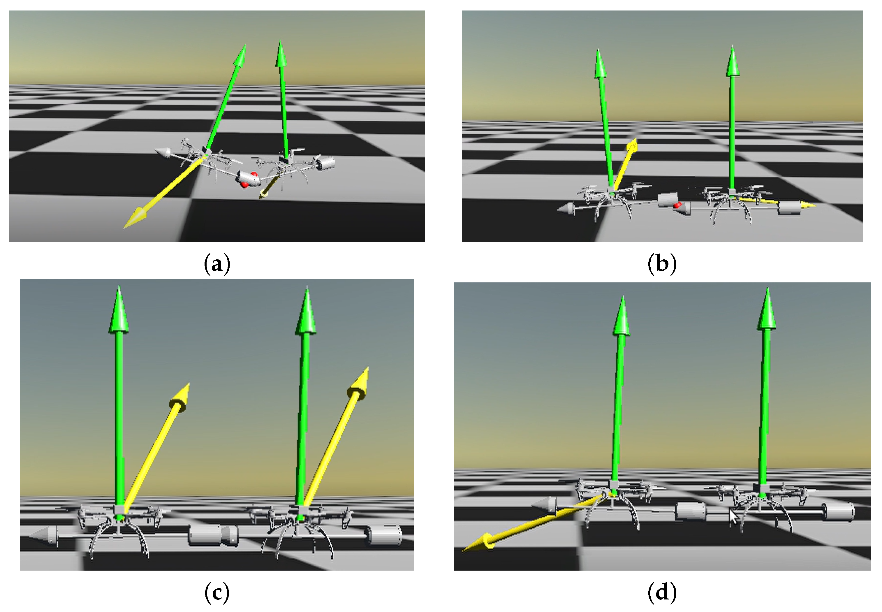
Figure 3 illustrates the various scenarios that may be encountered during the data collection process of expert policy in docking tasks. The success rate of the expert strategy in a noise-free environment is 40%. When collecting expert policy data, successful and unsuccessful data are of paramount importance. Successful data aids the model in learning how to make correct decisions to achieve the objective. Conversely, unsuccessful data helps the model understand which actions could lead to adverse outcomes, thereby avoiding the repetition of these errors in future decision-making. Therefore, whether it is successful or unsuccessful data, both are integral components of the learning and strategy optimization process in RL models.
We monitor the state of the two quadrotors in real time. If any anomalies are detected during the docking process, such as significant fluctuations in the roll angle or pitch angle, or a jamming situation caused by inaccurate docking angles between them, as shown in Figure 3a,b, we will terminate the current round of data collection with a heavy penalty and initiate the next episode.
In the control of quadrotors interacting with the external environment, the hybrid force/position control strategy provides an effective solution. This strategy allows quadrotors to accurately control the contact force while maintaining position control. In addition, through the switch of control modes, quadrotors can flexibly adjust their control strategies according to actual conditions. This method has strong adaptability and can adaptively adjust its motion trajectory to adapt to the actual situation. Finally, by inputting the ideal motion trajectory into the quadrotor’s attitude controller, trajectory and attitude tracking of the host can be achieved.
Our hybrid force/position control is only used on the docking axis. Because the external forces generated on the other two coordinate axes, apart from the docking axis, are relatively small. To simplify the process of generating contact external forces, we choose to temporarily ignore the external forces on the other two axes in the docking task. The docking work is not completed after the two quadrotors make contact. The completion of the docking work needs to be determined by the relative position and posture of the two quadrotors. To prevent the stability of the entire system from being affected by external forces after contact, we use hybrid force/position control after contact [53]. The formula is as follows:
where is the desired contact force in the world frame, is the real contact force, is the integral gains of the force control. It is important to note that our hybrid force/position control only acts on the y-axis, so the external forces in other directions are always set to zero.
During the data collection phase, the collected data includes the state of quadrotor A at time t , the state of quadrotor B at time t, , the six-dimensional contact forces . denotes the difference in target positions between quadrotor A and quadrotor B. The corresponding actions , , are the desired positions of quadrotor A and quadrotor B respectively at time t. , , , are the desired acceleration on the axis-z and the desired angle velocity of the quadrotor A and quadrotor B respectively.
3.2. Offline-to-Online Reinforcement Learning
We try to train the docking task directly through online RL, and the specific simulation result can be seen in Section 4.1. However, we find that using online RL directly can lead to catastrophic forgetting situations, and the overall docking task is difficult to train.
Online RL algorithms necessitate environmental exploration, which significantly increases training costs and reduces efficiency. When multiple tasks are present, the catastrophic forgetting of online RL complicates the entire training process. To address these issues, we attempted to accomplish the docking task directly through the offline RL approach. Experimental results indicate that this method is feasible. For the specific experimental process, please refer to Section 4.2. Further, based on the foundation of the offline RL model, we consider enhancing the model’s ability to explore the environment. Therefore, we integrate offline RL with online RL. The results prove that this method is indeed effective. For the specific result, please refer to Section 4.3.
Our algorithm framework is shown in Figure 4. In the pre-training phase, the TD3BC algorithm is utilized for training. The TD3BC algorithm, through state normalization, achieves enhanced stability. It stands out for its simplicity and efficiency, requiring only minor modifications to TD3 to achieve performance comparable to more complex methods. Subsequently, during the fine-tuning phase, we employ the PPO algorithm. Prior to the application of TD3BC, it is imperative to normalize the state, s, and the action, a, within the dataset as follows:
where and denote the mean and standard deviation of the i-th dimension of the dataset, respectively, is a small constant introduced to prevent division by zero, while represents the i-th dimension of either the state s or the action a.
The architecture we have devised facilitates the utilization of a shared actor network between the TD3BC and PPO algorithms. This is noteworthy given the fundamental divergence in their policy types: TD3BC employs a deterministic policy, while PPO utilizes a stochastic policy. The shared network comprises two hidden layers, with the first layer consisting of 512 neurons and the second layer containing 256 neurons. The rectified linear unit (ReLU) serves as the activation function. The network’s output is a normalized action, collectively forming an eight-dimensional vector. Notably, this output layer does not incorporate an activation function. The TD3BC critic network features two fully connected layers with 512 and 256 neurons, respectively, using the ReLU activation function. In contrast, the PPO critic network comprises three layers, each with 128 neurons, and utilizes the Leaky ReLU activation function.
The choice to abstain from utilizing the tanh activation function in the output layer is influenced by two primary considerations. Initially, due to the normalization procedure in Equation (9), it is not guaranteed that the output will fall within the −1 to 1 range. In fact, if the action space extends beyond the [−1, 1] interval, the tanh function will be incapable of representing actions outside this range. This could potentially restrict the expressiveness of the policy, thereby inhibiting the learned policy from executing certain possible actions. This is a crucial factor to consider in the design and implementation of RL algorithms. Secondly, the tanh function approaches a gradient near zero in its near-saturation regions, which is not conducive to fine-tuning in the PPO algorithm. This gradient could obstruct the effective learning and adjustment processes within PPO.
In the TD3BC algorithm, the computation of target actions, denoted as , is governed by the following formula:
where represents the target actor network, denotes the noise sampled from a normal distribution, c is the noise clip, and correspond to the minimum and maximum values of the action in the dataset, respectively.
In the PPO algorithm, the action that interacts with the environment is determined by the following expression:
where is the target actor network, is the noise scale.
The output of the actor network typically encompasses the mean and variance for action sampling within the PPO framework. However, the integration of the TD3BC pre-trained model as a guiding policy introduces complexity and limits control over the initial exploration intensity during the training phase. To mitigate this, we introduce as an independently trainable parameter, which is aligned with the dimensions of the action. This modification, which involves the integration of with the actor network, effectively shapes the stochastic policy within the PPO framework.
During the training process of PPO, we differentiate the state values given by the critic network and the actor network. This is primarily to balance the trade-off between exploration and exploitation, and to enhance the stability of the training. The critic network is mainly responsible for evaluating the performance of the current policy, typically through value function estimation. Therefore, it requires an accurate estimation of the environmental state to accurately evaluate the quality of the policy. Introducing noise into this process could potentially affect the accuracy of the value function, thereby impacting policy evaluation. On the other hand, the actor network is responsible for choosing actions based on the current state. Introducing noise into this process can increase the exploratory nature of the policy, enabling the agent to better explore the environment and identify potentially superior policies. Therefore, we do not add noise to the input state values on the critic network, while the state values on the actor network are noise-added. This design can balance the exploration-exploitation trade-off to a certain extent and improve the stability and effectiveness of the training.
3.3. Reward Function
In RL, the reward function plays a crucial role. It depends on the current state of the world, the action just taken, and the next state of the world. It can guide the agent’s behavior in order to maximize its long-term reward. We define the same reward function for both online and offline RL. During the process of collecting expert data, we found that the states of quadrotor A and quadrotor B have a significant impact on the entire docking process. Moreover, we aspire that the magnitude of external forces, once generated during the docking process, can provide some guidance to the entire procedure. This is to avert collision issues that could be caused by excessive external forces. So the reward function consists of four parts: attitude, position, guiding docking, and force reward.
The attitude reward function for quadrotors A and B is formulated as follows:
where is the trace of the rotation matrix R. The term represents the angle of rotation between the current orientation and the identity rotation matrix. We hope that during the docking process, the postures of the two quadrotors strive to maintain the form of the identity matrix.
For the position setting, we hope that the two quadrotors are as close as possible to their target positions. So the position reward function is defined as follows:
where is the current position of the quadrotor A, is the current position of the quadrotor B, is the target position of the quadrotor A.
We aim to enhance the stability during the docking process of two quadrotors. According to the data acquisition process of expert strategies, we find that the docking speed and accuracy have a significant impact on the successful completion of the docking task. Therefore, we add a guiding docking reward term in the entire reward function. This term can easily guide quadrotor B into the docking area, thereby greatly improving the docking success rate. As shown in Figure 1, when is in the guide area, the guiding reward will be added. The guiding docking reward function is defined as follows:
where represents the minimum reward, signifies the maximum reward, is the y-axis position of point , is the y-axis position of point .
For the force reward associated with contact forces, we aim to impose certain constraints on the docking forces along the y-axis. This is to prevent system instability issues that could arise from severe collisions. Therefore, the design of the force reward is as follows:
where and are the real contact force and desired contact force on the y-axis.
Consequently, the total reward function is articulated as follows:
where represent the weights assigned to the four types of rewards, is the time interval.
The allocation of reward weights in RL is a complex process. It should reflect the relative importance of various rewards to maintain balance. Through extensive experimentation and adjustment, we have determined the final allocation of reward weight parameters, as detailed in Table 1.
4. Simulation and Result
Our algorithm is available at AquaML [54]. The framework encompasses various online and offline RL algorithm frameworks and supports multi-machine parallel computation. The simulation environment is established in RaiSim. The operating frequency of the controller is 200 Hz. Our computational setup utilizes a CPU with 32 cores and 64 threads, and the GPU unit consists of 4 NVIDIA GeForce RTX 2080 Ti graphics cards.
4.1. Online RL Simulation
To accomplish the docking task, our initial approach is to employ online RL directly. Consequently, we experiment with various online RL methods. To evaluate the performance of these methods on the docking task, we adopt three different training strategies, as shown in Figure 5. In (a), we initially attempt to train using PPO directly. However, once the policy acquires the ability to control the movement of the two quadrotors, a collision between them results in a decrease in the accumulated reward, thereby impeding further learning.
To mitigate the issue of a sudden drop in reward due to collisions between two quadrotors, we propose dividing the docking task into two subtasks. The first subtask is stable flight (non-contact flight between two quadrotors), and the second subtask is to complete docking (stable flight after an external force is generated between two quadrotors). This approach aims to optimize the final task performance.
In Figure 5b,c, we employ a curriculum learning strategy, initially concentrating on training the agents to maneuver two quadrotors concurrently toward the desired position prior to docking. Following the successful completion of the first subtask, we then focus on optimizing the second subtask. (b) utilizes AMP, while (c) employs PPO. However, these methodologies fail to mitigate the negative impact of collisions on reward accumulation, leading to localized convergence during the training phase. The primary challenge in these scenarios is the compound nature of the task objectives, which significantly increases the risk of catastrophic forgetting.
4.2. Offline RL Simulation
During the offline RL phase, we employ 5000 complete docking trajectories. This phase is characterized by a rapid training speed that is completed in just half an hour.
We employ two types of offline RL methods, namely IQL and TD3BC. Both methods successfully complete the training. We conduct a comparative analysis of the success rates and time consumption of both methods. TD3BC achieves a success rate of 65% and requires 980 steps to complete the docking task, while IQL has a success rate of 60% and requires 990 steps. Therefore, for subsequent offline-to-online training, we utilize the model trained by TD3BC.
In the training process of TD3BC, many hyperparameters are indeed involved. The selection and adjustment of these hyperparameters have a significant impact on the performance of the model. Through algorithmic experience [33] and experiment, we can find the satisfactory hyperparameters, which are shown in Table 2.
4.3. Offline-to-Online RL Simulation
We choose to use offline-to-online RL. In the online RL phase, we deploy 21 processes, with 20 serving as sampling processes and one dedicated to policy updates. The entire training procedure spans 12 h, with the policy undergoing updates across 842 rounds. Each round samples 40,000 steps, culminating in a total of 34 million steps sampled throughout the training process.
In the fine-tuning process within the PPO framework, it is crucial to ensure that the divergence between the newly proposed and the existing policies does not exceed a certain threshold. This is to prevent instability during the policy update process, a key consideration in the design of the PPO algorithm. Firstly, if the difference between the old and new policies is too large, it could lead to instability in the training process or even a sharp decline in performance. By limiting the difference between the old and new policies, this situation can be avoided, thereby improving the stability of training. Secondly, in RL, a large step size in policy updates could lead to a “cliff fall” (i.e., obtaining a policy with poor performance), and it might take a long time or even be impossible to recover. By limiting the difference between the old and new policies, excessive updates can be avoided, thereby improving the efficiency of learning. Lastly, it has been found in practice that smaller policy updates are more likely to converge to the optimal solution during the training process. Excessive policy updates may cause the algorithm to oscillate near the optimal solution and not converge. Based on previous research experience [18,55] and our experiments, the hyperparameters are shown in Table 3. The proportion of old and new strategies is described in detail in Table 3 (target KL).
In our algorithm, we employ an early stop method, stopping the training process when the KL divergence exceeds 0.05. The parameters of PPO are selected based on the hyperparameter value of “log std init value” and have no connection with the original network. It serves as the variance of the Gaussian distribution for the PPO. To initiate effective training, the intensity of initial policy exploration should be moderate, with starting at −1.2 and gradually increasing throughout the training process. The entropy loss coefficient in PPO is configured to 0.005 to facilitate this gradual elevation in . As depicted in Figure 6b, the entropy value increases as the training progresses. Figure 6a illustrates the curve of the accumulated reward. We adopt a strategy that data collected during each update is randomly divided into four subsets, facilitating more efficient sample utilization. This approach, default in the AquaML framework, involves repeating the process 16 times, resulting in more stable training across various tasks. We perform an evaluation using the model derived from the 800th episode and attain a success rate of 95% within the docking environment.
In the quadrotor simulation, the incorporation of sensor noise is aimed at more realistically emulating the actual environment. In the real world, quadrotor sensor readings are often influenced by various factors, such as environmental interference and equipment errors, which result in a certain level of noise in the sensor readings. By introducing noise into the simulation, the simulated environment can be made to more closely resemble the actual operating environment, thereby enhancing the accuracy and reliability of the simulation. We obtain noise data by conducting multiple measurements on the sensor in the actual environment, recording the measurement values, and then analyzing the noise data through statistical methods. In the simulation process, based on experimental experience, we add independent Gaussian noise to the position and linear velocity data of the quadrotor state, as shown in Figure 7.
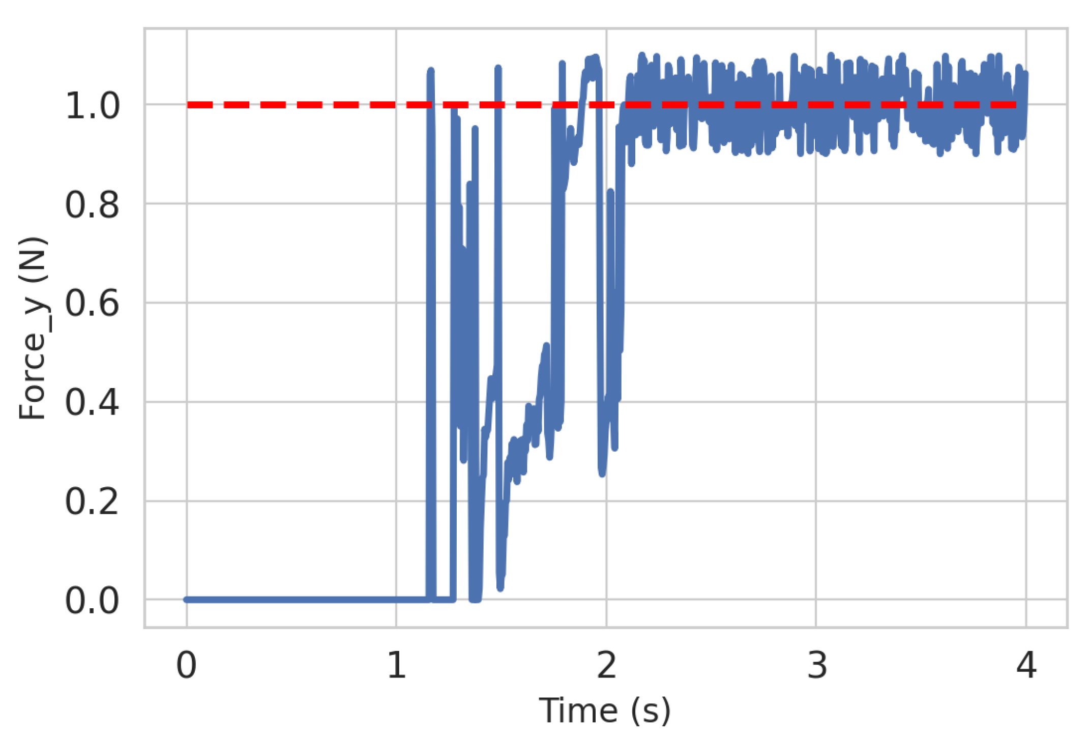
During the completion of the docking task, we simultaneously monitor the external forces generated between the two quadrotors. As time progresses, the quadrotors, while continuously approaching each other, generate external forces due to contact. Once fully docked, the external forces in the docking direction can be controlled within a certain range, as illustrated in Figure 8. And in this process, we are not using any force controller.
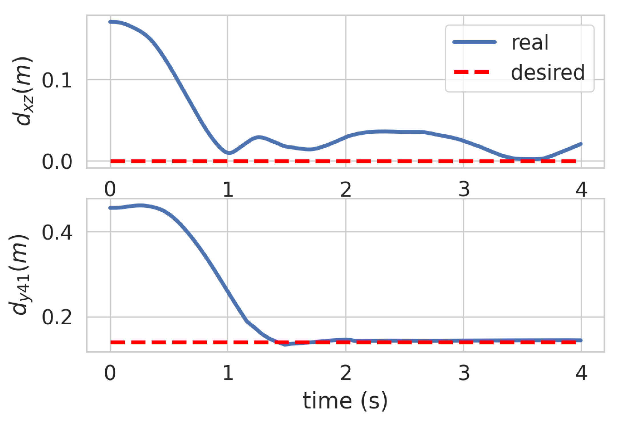
As depicted in Figure 9, the graph represents the variations in the distance, specifically on the plane and on the y-axis between points and , as shown in Figure 1. These distances pertain to the relative positioning of the two quadrotors during the docking process. When the complete coupling is achieved, the desired is set at m. This illustration substantiates that our approach proficiently administers the stable control of both the separation and complete docking processes of the two quadrotors.
The overall test results are shown in Table 4. In our test environment, each docking method is tested 200 times to calculate the success rate. The term ‘Steps’ refers to the average number of steps required to complete the docking task, which is derived based on a maximum step length of 2000. “AMP CL” represents the algorithm that combines AMP with course learning, “PPO CL” represents the algorithm that combines PPO with course learning, and × indicates training failure.
In the environmental setup, we also introduce randomness within a certain range for the initial relative pose of the two quadrotors. The initial position of quadrotor B is within a 1 m range to the right of the y-axis from the target position of quadrotor A. The initial position of quadrotor B is , and it is randomized within the following domain:
As demonstrated in Table 4, the offline-to-online algorithm achieves superior performance in terms of both success rate and time efficiency. Online RL is incapable of directly training for the docking task, whereas offline RL can accomplish task training. However, when comparing success rates and time consumption, offline RL still falls short of the offline-to-online method.
5. Conclusions
In this study, we proposed a scenario for quadrotor aerial docking tasks. The realization of this scenario allows quadrotors to complete free combination and separation tasks in the air, expanding the operational skills of quadrotors in complex scenarios. Firstly, we obtained better expert data by defining rules through traditional control methods. Secondly, we designed different RL methods to train the aerial docking tasks, including online RL, offline RL, and offline-to-online methods, and designed the reward function under the docking task. Ultimately, we used the offline-to-online method, TD3BC plus PPO, which achieved a success rate of 95% in the aerial docking scenario, outperforming other types of RL methods. This method can alleviate the problem of catastrophic forgetting in multi-task training scenarios to a certain extent, and mitigate the OOD problem in offline RL. It provides a promising direction for subsequent RL training with different types of task objectives.
For future work, we hope to deploy this scenario on real drones. Although the current success rate in the simulation environment has reached a high level, the transfer from simulation to reality is also a key issue we will consider in the future.
Author Contributions
Conceptualization, Y.Y.; Methodology, Y.F.; Validation, T.Y.; Investigation, Y.F.; Resources, Y.F.; Data curation, T.Y.; Writing—original draft, Y.F. and T.Y.; Writing—review and editing, Y.F. supervision, Y.Y. All authors have read and agreed to the published version of the manuscript.
Funding
This research was funded by the National Natural Science Foundation of China under Grant 62173037, the National Key R. D. Program of China, and the State Key Laboratory of Robotics and Systems (HIT).
Data Availability Statement
The following supporting information can be found at: https://drive.google.com/file/d/1k6SAxTvzHRVDskx8_wPrtFySkYnyJxr4/view?usp=drive_link (accessed on 10 April 2024), Video: Video of the UAV aerial docking.
Conflicts of Interest
The authors declare no conflict of interest.
References
- Karakostas, I.; Mademlis, I.; Nikolaidis, N.; Pitas, I. Shot type constraints in UAV cinematography for autonomous target tracking. Inf. Sci. 2020, 506, 273–294. [Google Scholar] [CrossRef]
- Shi, C.; Lai, G.; Yu, Y.; Bellone, M.; Lippiello, V. Real-Time Multi-Modal Active Vision for Object Detection on UAVs Equipped with Limited Field of View LiDAR and Camera. IEEE Robot. Autom. Lett. 2023, 8, 6571–6578. [Google Scholar] [CrossRef]
- Sharma, A.; Vanjani, P.; Paliwal, N.; Basnayaka, C.M.W.; Jayakody, D.N.K.; Wang, H.C.; Muthuchidambaranathan, P. Communication and networking technologies for UAVs: A survey. J. Netw. Comput. Appl. 2020, 168, 102739. [Google Scholar] [CrossRef]
- Yu, Y.; Wang, K.; Du, J.; Xu, B.; Xiang, C. Design and Trajectory Linearization Geometric Control of Multiple Aerial Vehicles Assembly. J. Mech. Eng. 2022, 58, 16–26. [Google Scholar] [CrossRef]
- Nguyen, H.N.; Park, S.; Park, J.; Lee, D. A novel robotic platform for aerial manipulation using quadrotors as rotating thrust generators. IEEE Trans. Robot. 2018, 34, 353–369. [Google Scholar] [CrossRef]
- Yu, Y.; Shi, C.; Shan, D.; Lippiello, V.; Yang, Y. A hierarchical control scheme for multiple aerial vehicle transportation systems with uncertainties and state/input constraints. Appl. Math. Model. 2022, 109, 651–678. [Google Scholar] [CrossRef]
- Sanalitro, D.; Savino, H.J.; Tognon, M.; Cortés, J.; Franchi, A. Full-Pose Manipulation Control of a Cable-Suspended Load with Multiple UAVs Under Uncertainties. IEEE Robot. Autom. Lett. 2020, 5, 2185–2191. [Google Scholar] [CrossRef]
- Park, S.; Lee, Y.; Heo, J.; Lee, D. Pose and Posture Estimation of Aerial Skeleton Systems for Outdoor Flying. In Proceedings of the 2019 International Conference on Robotics and Automation (ICRA), Montreal, QC, Canada, 20–24 May 2019; pp. 704–710. [Google Scholar] [CrossRef]
- Park, S.; Lee, J.; Ahn, J.; Kim, M.; Her, J.; Yang, G.H.; Lee, D. ODAR: Aerial Manipulation Platform Enabling Omnidirectional Wrench Generation. IEEE/ASME Trans. Mechatron. 2018, 23, 1907–1918. [Google Scholar] [CrossRef]
- Sugihara, J.; Nishio, T.; Nagato, K.; Nakao, M.; Zhao, M. Design, Control, and Motion Strategy of TRADY: Tilted-Rotor-Equipped Aerial Robot with Autonomous In-flight Assembly and Disassembly Ability. arXiv 2023, arXiv:2303.07106. [Google Scholar]
- Zhang, M.; Li, M.; Wang, K.; Yang, T.; Feng, Y.; Yu, Y. Zero-Shot Sim-To-Real Transfer of Robust and Generic Quadrotor Controller by Deep Reinforcement Learning. In Proceedings of the International Conference on Cognitive Systems and Signal Processing, LuoYang, China, 10–12 August 2023; Springer: Berlin/Heidelberg, Germany, 2023; pp. 27–43. [Google Scholar]
- Feng, Y.; Shi, C.; Du, J.; Yu, Y.; Sun, F.; Song, Y. Variable admittance interaction control of UAVs via deep reinforcement learning. In Proceedings of the 2023 IEEE International Conference on Robotics and Automation (ICRA), London, UK, 29 May–2 June 2023; IEEE: Piscataway, NJ, USA, 2023; pp. 1291–1297. [Google Scholar]
- Song, Y.; Romero, A.; Müller, M.; Koltun, V.; Scaramuzza, D. Reaching the limit in autonomous racing: Optimal control versus reinforcement learning. Sci. Robot. 2023, 8, eadg1462. [Google Scholar] [CrossRef]
- Kaufmann, E.; Bauersfeld, L.; Loquercio, A.; Müller, M.; Koltun, V.; Scaramuzza, D. Champion-level drone racing using deep reinforcement learning. Nature 2023, 620, 982–987. [Google Scholar] [CrossRef] [PubMed]
- Schulman, J.; Wolski, F.; Dhariwal, P.; Radford, A.; Klimov, O. Proximal policy optimization algorithms. arXiv 2017, arXiv:1707.06347. [Google Scholar]
- Chikhaoui, K.; Ghazzai, H.; Massoud, Y. PPO-based reinforcement learning for UAV navigation in urban environments. In Proceedings of the 2022 IEEE 65th International Midwest Symposium on Circuits and Systems (MWSCAS), Fukuoka, Japan, 7–10 August 2022; IEEE: Piscataway, NJ, USA, 2022; pp. 1–4. [Google Scholar]
- Guan, Y.; Zou, S.; Peng, H.; Ni, W.; Sun, Y.; Gao, H. Cooperative UAV trajectory design for disaster area emergency communications: A multi-agent PPO method. IEEE Internet Things J. 2023, 11, 8848–8859. [Google Scholar] [CrossRef]
- Molchanov, A.; Chen, T.; Hönig, W.; Preiss, J.A.; Ayanian, N.; Sukhatme, G.S. Sim-to-(multi)-real: Transfer of low-level robust control policies to multiple quadrotors. In Proceedings of the 2019 IEEE/RSJ International Conference on Intelligent Robots and Systems (IROS), Macao, China, 3–8 November 2019; IEEE: Piscataway, NJ, USA, 2019; pp. 59–66. [Google Scholar]
- Vithayathil Varghese, N.; Mahmoud, Q.H. A survey of multi-task deep reinforcement learning. Electronics 2020, 9, 1363. [Google Scholar] [CrossRef]
- Abbeel, P.; Ng, A.Y. Apprenticeship learning via inverse reinforcement learning. In Proceedings of the Twenty-First International Conference on Machine Learning, New York, NY, USA, 4 July 2004; p. 1. [Google Scholar]
- Ziebart, B.D.; Maas, A.L.; Bagnell, J.A.; Dey, A.K. Maximum entropy inverse reinforcement learning. In Proceedings of the AAAI, Chicago, IL, USA, 13–17 July 2008; Volume 8, pp. 1433–1438. [Google Scholar]
- Arora, S.; Banerjee, B.; Doshi, P. Maximum Entropy Multi-Task Inverse RL. arXiv 2020, arXiv:2004.12873. [Google Scholar]
- Ho, J.; Ermon, S. Generative adversarial imitation learning. In Advances in Neural Information Processing Systems 29, Proceedings of the 30th Annual Conference on Neural Information Processing Systems 2016, Barcelona, Spain, 5–10 December 2016; NeurIPS: La Jolla, CA, USA, 2016. [Google Scholar]
- Peng, X.B.; Ma, Z.; Abbeel, P.; Levine, S.; Kanazawa, A. Amp: Adversarial motion priors for stylized physics-based character control. ACM Trans. Graph. (ToG) 2021, 40, 1–20. [Google Scholar] [CrossRef]
- Vollenweider, E.; Bjelonic, M.; Klemm, V.; Rudin, N.; Lee, J.; Hutter, M. Advanced skills through multiple adversarial motion priors in reinforcement learning. In Proceedings of the 2023 IEEE International Conference on Robotics and Automation (ICRA), London, UK, 29 May–2 June 2023; IEEE: Piscataway, NJ, USA, 2023; pp. 5120–5126. [Google Scholar]
- Wu, J.; Xin, G.; Qi, C.; Xue, Y. Learning robust and agile legged locomotion using adversarial motion priors. IEEE Robot. Autom. Lett. 2023, 8, 4975–4982. [Google Scholar] [CrossRef]
- Pomerleau, D.A. Efficient training of artificial neural networks for autonomous navigation. Neural Comput. 1991, 3, 88–97. [Google Scholar] [CrossRef] [PubMed]
- Torabi, F.; Warnell, G.; Stone, P. Behavioral cloning from observation. arXiv 2018, arXiv:1805.01954. [Google Scholar]
- Kumar, A.; Hong, J.; Singh, A.; Levine, S. Should i run offline reinforcement learning or behavioral cloning? In Proceedings of the International Conference on Learning Representations, Virtual, 25–29 April 2022. [Google Scholar]
- Yang, J.; Zhou, K.; Li, Y.; Liu, Z. Generalized out-of-distribution detection: A survey. arXiv 2021, arXiv:2110.11334. [Google Scholar]
- Levine, S.; Kumar, A.; Tucker, G.; Fu, J. Offline reinforcement learning: Tutorial, review, and perspectives on open problems. arXiv 2020, arXiv:2005.01643. [Google Scholar]
- Kumar, A.; Zhou, A.; Tucker, G.; Levine, S. Conservative q-learning for offline reinforcement learning. Adv. Neural Inf. Process. Syst. 2020, 33, 1179–1191. [Google Scholar]
- Fujimoto, S.; Gu, S.S. A minimalist approach to offline reinforcement learning. Adv. Neural Inf. Process. Syst. 2021, 34, 20132–20145. [Google Scholar]
- Agarwal, R.; Schuurmans, D.; Norouzi, M. An optimistic perspective on offline reinforcement learning. In Proceedings of the International Conference on Machine Learning (PMLR), Virtual, 13–18 July 2020; pp. 104–114. [Google Scholar]
- Kostrikov, I.; Nair, A.; Levine, S. Offline reinforcement learning with implicit q-learning. arXiv 2021, arXiv:2110.06169. [Google Scholar]
- Fujimoto, S.; Meger, D.; Precup, D. Off-policy deep reinforcement learning without exploration. In Proceedings of the International conference on machine learning (PMLR), Long Beach, CA, USA, 9–15 June 2019; pp. 2052–2062. [Google Scholar]
- Ghasemipour, S.K.S.; Schuurmans, D.; Gu, S.S. Emaq: Expected-max q-learning operator for simple yet effective offline and online rl. In Proceedings of the International Conference on Machine Learning (PMLR), Virtual, 18–24 July 2021; pp. 3682–3691. [Google Scholar]
- Jaques, N.; Ghandeharioun, A.; Shen, J.H.; Ferguson, C.; Lapedriza, A.; Jones, N.; Gu, S.; Picard, R. Way off-policy batch deep reinforcement learning of implicit human preferences in dialog. arXiv 2019, arXiv:1907.00456. [Google Scholar]
- Kumar, A.; Fu, J.; Soh, M.; Tucker, G.; Levine, S. Stabilizing off-policy q-learning via bootstrapping error reduction. In Advances in Neural Information Processing Systems 32, Proceedings of the 33rd Conference on Neural Information Processing Systems (NeurIPS 2019), Vancouver, Canada, 8–14 December 2019; NeurIPS: La Jolla, CA, USA, 2019. [Google Scholar]
- Wu, Y.; Tucker, G.; Nachum, O. Behavior regularized offline reinforcement learning. arXiv 2019, arXiv:1911.11361. [Google Scholar]
- Siegel, N.Y.; Springenberg, J.T.; Berkenkamp, F.; Abdolmaleki, A.; Neunert, M.; Lampe, T.; Hafner, R.; Heess, N.; Riedmiller, M. Keep doing what worked: Behavioral modelling priors for offline reinforcement learning. arXiv 2020, arXiv:2002.08396. [Google Scholar]
- Guo, Y.; Feng, S.; Le Roux, N.; Chi, E.; Lee, H.; Chen, M. Batch reinforcement learning through continuation method. In Proceedings of the International Conference on Learning Representations, Virtual, 3–7 April 2020. [Google Scholar]
- Hwangbo, J.; Lee, J.; Hutter, M. Per-contact iteration method for solving contact dynamics. IEEE Robot. Autom. Lett. 2018, 3, 895–902. [Google Scholar] [CrossRef]
- Quan, Q. Introduction to Multicopter Design and Control; Springer: Berlin/Heidelberg, Germany, 2017. [Google Scholar]
- Fahad Mon, B.; Wasfi, A.; Hayajneh, M.; Slim, A.; Abu Ali, N. Reinforcement Learning in Education: A Literature Review. Informatics 2023, 10, 74. [Google Scholar] [CrossRef]
- Sivamayil, K.; Rajasekar, E.; Aljafari, B.; Nikolovski, S.; Vairavasundaram, S.; Vairavasundaram, I. A Systematic Study on Reinforcement Learning Based Applications. Energies 2023, 16, 1512. [Google Scholar] [CrossRef]
- Sutton, R.S.; Barto, A.G. Reinforcement Learning: An Introduction; MIT Press: Cambridge, MA, USA, 2018. [Google Scholar]
- Pinosky, A.; Abraham, I.; Broad, A.; Argall, B.; Murphey, T.D. Hybrid control for combining model-based and model-free reinforcement learning. Int. J. Robot. Res. 2023, 42, 337–355. [Google Scholar] [CrossRef]
- Byeon, H. Advances in Value-based, Policy-based, and Deep Learning-based Reinforcement Learning. Int. J. Adv. Comput. Sci. Appl. 2023, 14, 348–354. [Google Scholar] [CrossRef]
- Wang, X.; Wang, S.; Liang, X.; Zhao, D.; Huang, J.; Xu, X.; Dai, B.; Miao, Q. Deep Reinforcement Learning: A Survey. IEEE Trans. Neural Netw. Learn. Syst. 2024, 35, 5064–5078. [Google Scholar] [CrossRef]
- Yi, W.; Qu, R.; Jiao, L. Automated algorithm design using proximal policy optimisation with identified features. Expert Syst. Appl. 2023, 216, 119461. [Google Scholar] [CrossRef]
- Nguyen, H.N.; Lee, D. Hybrid force/motion control and internal dynamics of quadrotors for tool operation. In Proceedings of the 2013 IEEE/RSJ International Conference on Intelligent Robots and Systems, Tokyo, Japan, 3–7 November 2013; IEEE: Piscataway, NJ, USA, 2013; pp. 3458–3464. [Google Scholar]
- Nguyen, H.N.; Ha, C.; Lee, D. Mechanics, control and internal dynamics of quadrotor tool operation. Automatica 2015, 61, 289–301. [Google Scholar] [CrossRef]
- Tao, Y.; Yu, Y.; Feng, Y. AqauML: Distributed Deep Learning Framework Based on Tensorflow2. 2023. Available online: https://github.com/BIT-aerial-robotics/AquaML/tree/2.2.0 (accessed on 2 May 2023).
- Huang, S.; Dossa, R.F.J.; Raffin, A.; Kanervisto, A.; Wang, W. The 37 implementation details of proximal policy optimization. In Proceedings of the The ICLR Blog Track, Online, 25–29 April 2022. [Google Scholar]
Figure 1.
This is a schematic diagram of the docking structure. is the distance between and on the y-axis, is the distance between and on the -axis. is the depth of quadrotor A docking device, is the length of quadrotor B docking device, is the length of Guide area, and is the diameter of the barrel.

Figure 2.
Flowchart of the rule-based expert policy. Initially, quadrotor A remains hovering, while quadrotor B gradually approaches quadrotor A along the y-axis. If contact occurs between the two, it is determined whether the docking conditions (tip is in recess) are met. If they are, force-position hybrid control can be implemented until the target point is reached and docking is completed. If the conditions are not met, to avoid becoming stuck, quadrotor B needs to move back to ensure the disappearance of external forces, and then approach quadrotor A along the y-axis.

Figure 3.
The potential interaction process of expert policy within RaiSim. The green arrow points in the direction of the resultant force, while the yellow arrow points in the direction of the resultant torque. (a,b) illustrate potential scenarios where two quadrotors may become stuck during the docking process; (c,d) depict two scenarios that may occur when two quadrotors successfully dock.

Figure 4.
Flowchart of the proposed method. The far left represents the process of collecting data from expert policy. The expert policy comprises a PID controller and a hybrid force/position controller, which are switched and adapted to alter the desired poses of the two quadrotors based on a series of predetermined rules. The policy outputs thrust and angular velocity, which are processed by a thrust-omega controller to generate the thrust values for the four motors of the quadrotor. The four thrust values are then applied to the quadrotor in the RaiSim environment, thereby driving the quadrotor to execute maneuvers. The middle diagram represents the offline RL, which uses TD3BC for training based on the data collected from the expert strategy. And the MLP is a multi-layered perceptron. Finally, in the far right diagram, PPO is used for online fine-tuning.

Figure 5.
The accumulated rewards are trained via Online RL; (a) is the reward by PPO; (b) is the reward of curriculum learning and AMP; and (c) is the reward of curriculum learning and PPO.
Figure 5.
The accumulated rewards are trained via Online RL; (a) is the reward by PPO; (b) is the reward of curriculum learning and AMP; and (c) is the reward of curriculum learning and PPO.

Figure 6.
Accumulated reward and entropy curve in the fine-tuning phase; (a) shows the accumulated reward during the fine-tuning phase; (b) represents the entropy curve in the fine-tuning phase.
Figure 6.
Accumulated reward and entropy curve in the fine-tuning phase; (a) shows the accumulated reward during the fine-tuning phase; (b) represents the entropy curve in the fine-tuning phase.

Figure 7.
Gaussian noise is incorporated into the state measurements. (a) shows the noise and target values of position; (b) represents the noise and target values of linear velocity. The solid blue line represents the noise in the position and linear velocity. The dashed red line indicates the target values.

Figure 8.
Throughout the completion of the docking task, the external force values generated on the y-axis are tracked. The dashed red line represents the target external force values, while the solid blue line represents the actual values.
Figure 8.
Throughout the completion of the docking task, the external force values generated on the y-axis are tracked. The dashed red line represents the target external force values, while the solid blue line represents the actual values.

Figure 9.
The changes of and during docking. The dashed red line represents the ideal value at complete docking and the solid blue line is the real value.
Figure 9.
The changes of and during docking. The dashed red line represents the ideal value at complete docking and the solid blue line is the real value.


Table 1.
Reward function parameters.
| Parameter | Value |
|---|---|
| 0.1 | |
| 1.02 | |
| 1.0 | |
| 0.3 | |
| 2.0 | |
| 0.0 | |
| 0.02 |
Table 2.
TD3BC hyperparameters.
| Parameter | Value |
|---|---|
| Batch size | 4096 |
| Target update rate | 0.005 |
| Policy noise | 0.2 |
| Policy noise clipping | (−0.5, 0.5) |
| Policy update frequency | 2 |
| Actor learning rate | 3 × 10⁻⁴ |
| 2.5 |
Table 3.
PPO hyperparameters.
| Parameter | Value |
|---|---|
| 0.99 | |
| clip ratio | 0.05 |
| target KL | 0.05 |
| log std init value | −1.2 |
| 1.0 | |
| entropy coef | 0.005 |
| learning rate | 2 × 10⁻⁶ |
Table 4.
Algorithm performance comparison for aerial docking task.
| Algorithm Type | Algorithm | Success Rate | Steps |
|---|---|---|---|
| Online | PPO | × | × |
| Online | AMP CL | × | × |
| Online | PPO CL | × | × |
| Offline | IQL | 60% | 990 |
| Offline | TD3BC | 65% | 980 |
| Offline-to-Online | TD3BC+PPO | 95% | 890 |
Disclaimer/Publisher’s Note: The statements, opinions and data contained in all publications are solely those of the individual author(s) and contributor(s) and not of MDPI and/or the editor(s). MDPI and/or the editor(s) disclaim responsibility for any injury to people or property resulting from any ideas, methods, instructions or products referred to in the content. |
© 2024 by the authors. Licensee MDPI, Basel, Switzerland. This article is an open access article distributed under the terms and conditions of the Creative Commons Attribution (CC BY) license (https://creativecommons.org/licenses/by/4.0/).
Share and Cite
MDPI and ACS Style
Feng, Y.; Yang, T.; Yu, Y. Enhancing UAV Aerial Docking: A Hybrid Approach Combining Offline and Online Reinforcement Learning. Drones 2024, 8, 168. https://doi.org/10.3390/drones8050168
AMA Style
Feng Y, Yang T, Yu Y. Enhancing UAV Aerial Docking: A Hybrid Approach Combining Offline and Online Reinforcement Learning. Drones. 2024; 8(5):168. https://doi.org/10.3390/drones8050168
Chicago/Turabian StyleFeng, Yuting, Tao Yang, and Yushu Yu. 2024. "Enhancing UAV Aerial Docking: A Hybrid Approach Combining Offline and Online Reinforcement Learning" Drones 8, no. 5: 168. https://doi.org/10.3390/drones8050168