Cruciform Specimen Design for Biaxial Tensile Testing of SMC

Abstract

This paper presents an investigation of different cruciform specimen designs for the characterization of sheet molding compound (SMC) under biaxial loading. The considered material is a discontinuous glass fiber reinforced thermoset. We define various (material-specific) requirements for an optimal specimen design. One key challenge represents the achievement of a high strain level in the center region of the cruciform specimen in order to observe damage, at the same time prevention of premature failure in the clamped specimen arms. Starting from the ISO norm for sheet metals, we introduce design variations, including two concepts to reinforce the specimens’ arms. An experimental evaluation includes two different loading scenarios, uniaxial tension and equi-biaxial tension. The best fit in terms of the defined optimality criteria, is a specimen manufactured in a layup with unidirectional reinforcing outer layers where a gentle milling process exposed the pure SMC in the center region of the specimen. This specimen performed superior for all considered loading conditions, for instance, in the uniaxial loading scenario, the average strain in the center region reached $87\%$ of the failure strain in a uniaxial tensile bone specimen.

1. Introduction

1.1. Motivation

With their high mass-specific strength and stiffness, fiber reinforced polymers receive considerable attention in mass-reduction strategies in the automotive and aerospace sector. The stiffest and strongest class of composites are continuous fiber reinforced composites. This work, however, focuses on discontinuous fiber reinforced composites in form of sheet molding compounds (SMCs). SMCs offer a large freedom of design and the low cycle times allow for mass production. Characteristics of SMC include brittleness, process-induced inhomogeneity and anisotropy, and comparably large microstructure dimensions.

The application of SMC is hindered by the lack of a precise understanding of its mechanical behavior. The focus of the present work lies in biaxial tensile testing of SMC, which is driven by two main factors. Firstly, the characterization under biaxial stress states covers a wide range of application loads on typical shell-like SMC structures. Secondly, as the implementation of virtual process chains and, especially, damage modeling increases in popularity, a detailed characterization of the damage behavior is essential to understand the complex damage phenomena and calibrate corresponding constitutive models. For instance, biaxial tensile testing allows for a validation of the anisotropic evolution of stiffness.

The cruciform specimen design significantly influences the characterization range of stress states as well as the precision of the characterized material properties. Optimization of specimen design is a material-dependent multi-objective task.

1.2. State-of-the-Art

In the past, many attempts have been made to find an appropriate cruciform specimen design, demonstrating that the specimen design is one of the most challenging aspects of the biaxial testing. Several authors have proposed specimen designs for specific applications and materials, varying the cut shape, the type of the thickness-reduced area and the type of slits in the specimen arms, which serve to reduce undesired lateral constraints on the strain in the center region of the specimen [1]. Deng et al. [2], Kuwabara et al. [3] and Makinde et al. [4] optimized specimens for metals. Demmerle and Boehler [5] compared different proposed specimen designs and chose the specimen of Kelly [6] with slits and a thickness reduced area to perform an optimization for isotropic materials. Boehler et al. [7] investigated anisotropic sheet metals with this specimen type. Hoferlin et al. [8] presented an alternative specimen design with slits and reinforced arms. Hannon and Tiernan [9] reviewed planar biaxial tensile test systems for sheet metals. ISO 16842 [10] is the first standardization in this field but applies to sheet metals only. Green et al. [11] proposed a sandwich design for aluminum sheet alloys in which the sample sheet is bonded by an adhesive between two face sheets, while leaving the center region free on both sides.

Other authors conducted research to find a suitable specimen for composites and polymers. Smits et al. [12] and Van Hemelrijck et al. [13] investigated the influence of parameters like the radius of the corner fillet and the thickness and the geometry of the biaxially loaded area by finite element simulations and experiments. This investigation led to a suitable specimen for fiber reinforced composite laminates with a reduced thickness area in the center region of the specimen, in combination with a fillet corner between arms. Makris et al. [14] and Makinde et al. [4] optimized the specimen shape by a numerical optimization technique with a parametric finite element model. Lamkanfi et al. [15] and Gower and Shaw [16] showed that geometrical discontinuities like the transition zone to the tapered thickness area have a major influence on the strain distribution leading to premature failure. Serna Moreno et al. [17] compared specimens with arms of different widths for chopped glass-reinforced polyester. They presented a specimen that was suitable to achieve failure in the center area in different loading cases but pointed out that there are still problems such as stress concentrations outside the center area. This glance into the literature shows that, despite the promising improvements already achieved, there are still many challenges ahead in the search for suitable cruciform specimen designs for composites.

1.3. Present Work

This work presents an investigation of different specimen designs for biaxial tensile testing of SMC. We aim for an optimal geometry for the characterization of damage evolution under a wide range of biaxial planar stress states. The outline is as follows: Section 2.2 presents the background of biaxial tensile testing and introduces the two loading scenarios we apply for the experimental evaluation of the specimen design. Section 3 begins with a definition of our specific specimen optimality criteria. In the following, we introduce four specimen designs and evaluate them experimentally and partly with finite element simulations. Section 4 discusses and compares the results in terms of the introduced optimality criteria.

2. Materials and Experiment

2.1. Materials and Manufacturing Process

The SMC considered here consists, specifically, of an unsaturated polyester polyurethane hybrid (UPPH) matrix system, reinforced with $23\mathrm{vol}\%$ glass fibers. The SMC was manufactured at the Fraunhofer Institute of Chemical Technology (ICT) at Pfinztal, Germany. The detailed composition of the matrix system is listed in

Table 1. Composition of the unsaturated polyester polyurethane hybrid (UPPH) resin [18].

Component	Trade Name	Weight Fraction
UPPH resin	Daron ZW 14142	$77\%$
Adherent and flow aids	BYK 9085	$1.5\%$
Impregnation aid	BYK 9076	$2.3\%$
Deaeration aid	BYK A-530	$0.38\%$
Inhibitor	pBQ	$0.0023\%$
Peroxide	Trigonox 117	$0.77\%$
Isocyanate	Lupranat M20R	$18\%$

. The length of the fibers is $25.4\mathrm{mm}$.

The SMC pre-impregnated fibers were manufactured on a belt conveyor system. The initial charge had $60\%$ mold coverage (with exception of the specimens presented in Section 3.4) in a square mold with the dimensions $455\times 455\mathrm{mm}$ and consisted of three layers of pre-impregnated fibers. With regard to more details of the manufacturing process, we refer to [18]. All specimens were cut with a water jet cutter from the center region of the plate to minimize the influence of inhomogeneous fiber dispersion, e.g., investigated in [19].

2.2. Biaxial Tensile Experiments

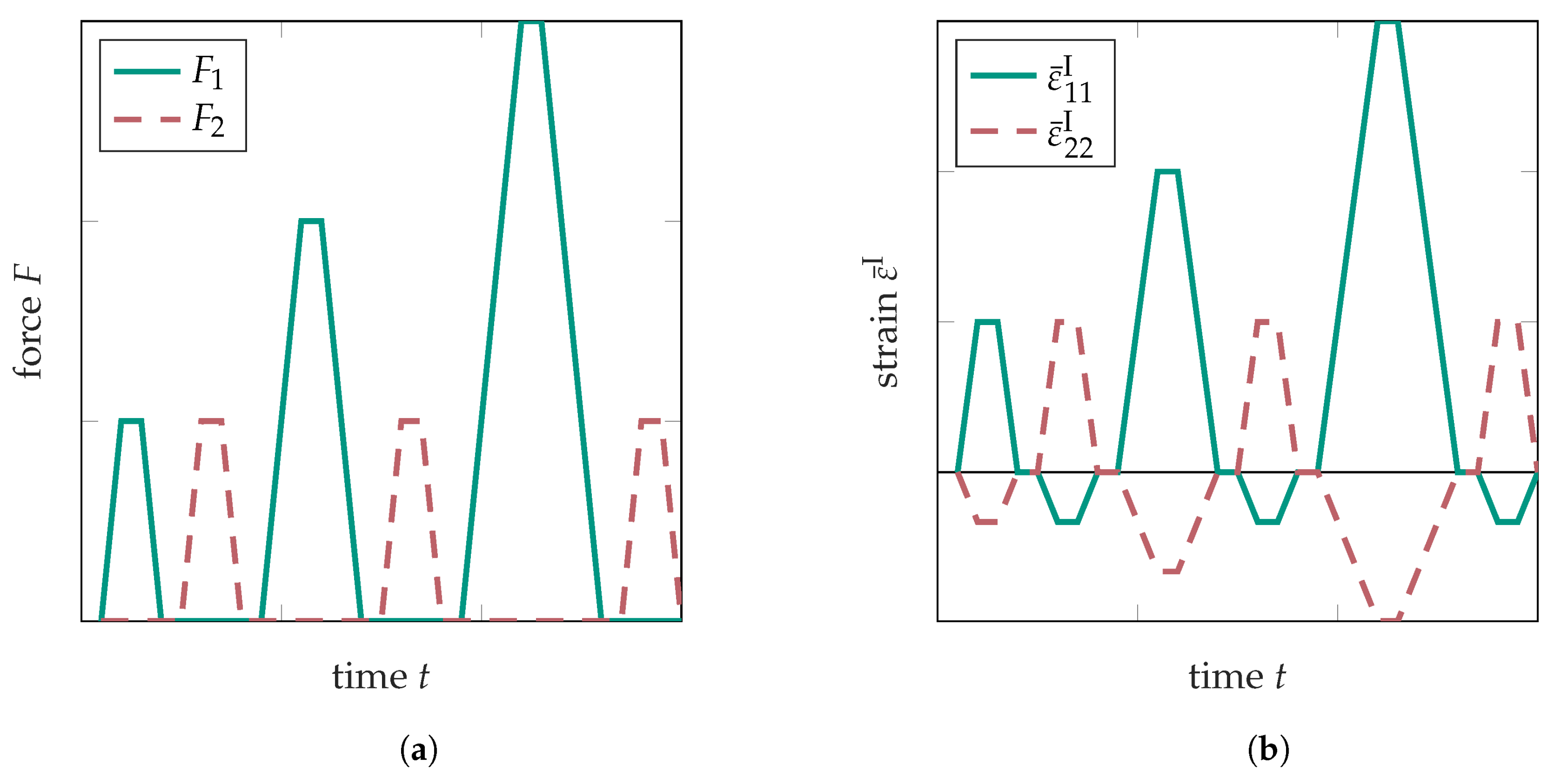
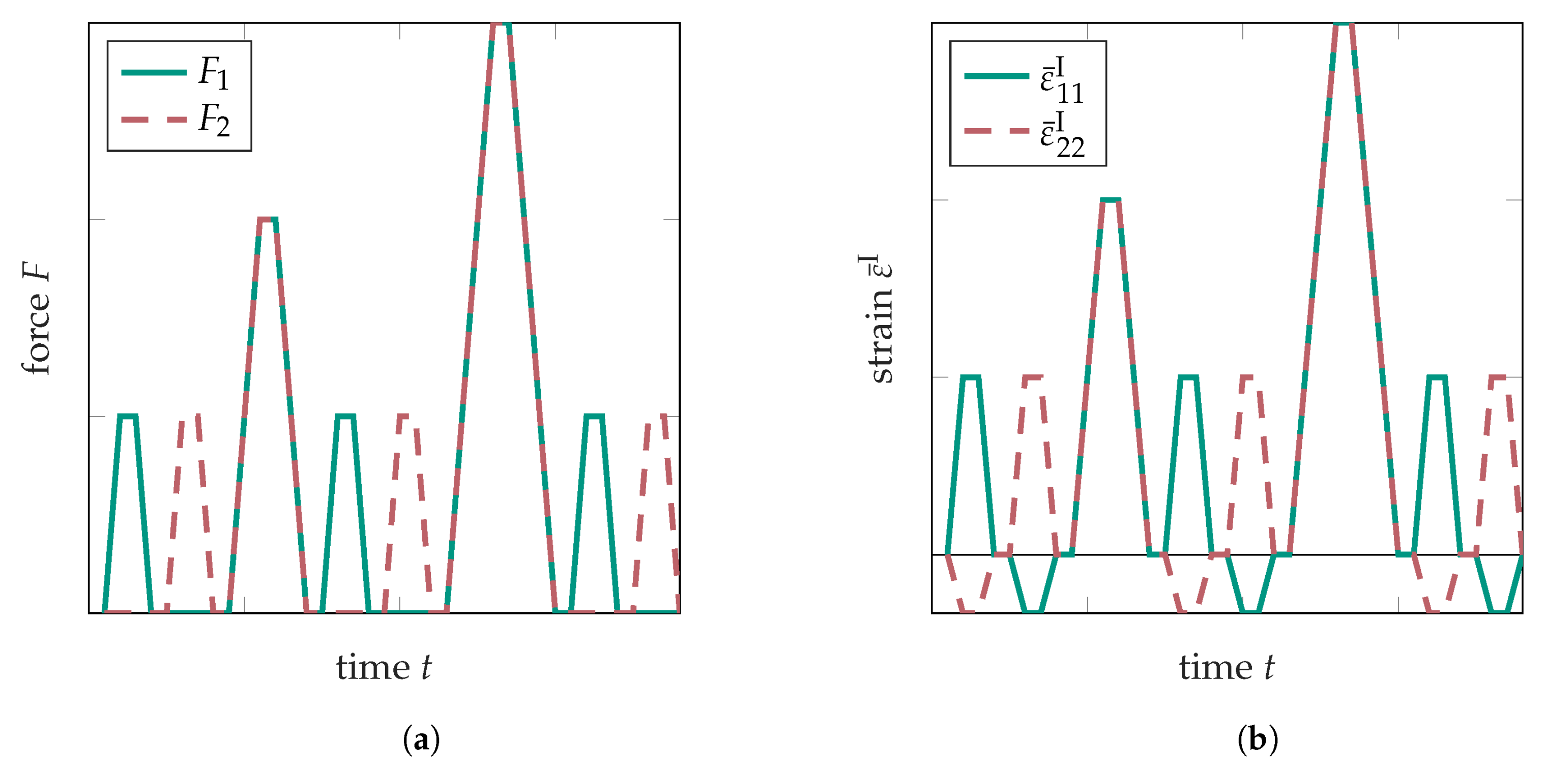
2.2.1. Fundamentals of Biaxial Tensile Testing

In this section, we briefly introduce our biaxial tensile testing device at the Institute of Engineering Mechanics (KIT) and some fundamentals on biaxial tensile testing. The biaxial tensile testing device shown in Figure 1a consists of four horizontally positioned elctro-mechanical actuators that are arranged perpendicular to each other. Each axis allows for a maximum load of $150\mathrm{kN}$ and is equipped with a load cell. The deformation of the specimen is measured by an integrated optical strain measurement system via the displacement of five points on the bottom of the specimen. The movement of these points is the input for the measurement of the strain load and midpoint control. The active midpoint control allows for bending-free load applications, even in the case of heterogeneous specimens. On the upper side of the specimen, a speckle pattern allows for full field strain measurements via digital image correlation. Due to the, in general, inhomogeneous stress and strain fields in the cruciform specimens the parameter identification is typically not as straightforward as, e.g., in uniaxial tensile tests. More details concerning inverse parameter identification are, e.g., covered in [20,21,22,23,24,25].

Figure 1b depicts an exemplary cruciform specimen. If we assume the specimen as homogeneous, the opposing forces on the specimen are equal and given by $F_1$ in positive and negative $e_1$-direction and $F_2$ in positive and negative $e_2$-direction. The ratio of these two forces is known as the loading ratio

$$\Gamma ={\displaystyle \frac{F_2}{F_1}}.$$

(1)

The loading ratio of $\Gamma =0$ defines uniaxial tension or compression in the $e_1$-direction, whereas the loading ratio $\Gamma =1$ defines equi-biaxial tension or compression. We define the area of interest $A^{\mathrm{I}}$ as the measuring region which later can serve as input for the parameter identification. In all following contour plots, the area of interest is highlighted by a purple frame. For the cruciform specimen design, the area-averaged strain over the area of interest,

$${\overline{\epsilon }}_{ij}^{\mathrm{I}}={\displaystyle \frac{1}{A^{\mathrm{I}}}}{\int }_{A^{\mathrm{I}}}{\epsilon }_{ij}\left(\mathit{x}\right)\mathrm{d}A,$$

(2)

is a key quantity in the evaluation of the specimen geometries, with ${\epsilon }_{ij}=\left(\partial u_i/\partial x_j+\partial u_j/\partial x_i\right)/2$ being the components of the infinitesimal strain tensor defined from the displacement vector $u_i$.

2.2.2. Experimental Procedures

For the experimental and simulative evaluation of the specimen designs, we focus on two loading scenarios. We avoid compressive loads as they may lead to buckling issues. The distinction of the mechanical phenomena like, for instance, elasticity, stiffness degradation (damage), plasticity, and viscoelasticity is simplified by a stepwise load application and waiting times between the load application steps.

The first procedure $P_{\Gamma =0}$ is based on cyclic uniaxial tension in $e_1$-direction with a stepwise load increase. Between these loading steps, we apply a constant uniaxial tension in the $e_2$-direction. This allows for an observation of stiffness degradation in and perpendicular to the main loading direction. Figure 2 shows a schematic stress and strain path for the loading procedure $P_{\Gamma =0}$. The tensile load is applied strain-controlled. Perpendicular to the respective loading direction, a force control ensures a low contact force.

The second procedure $P_{\Gamma =1}$ (see Figure 3) is designed such that the damage inducing load is equi-biaxial tension. Between the biaxial tension steps of increasing amplitude, uniaxial tension steps of small and constant amplitude are applied in the $e_1$-direction and subsequently in the $e_2$-direction in order to estimate the stiffness evolution in these directions. The strain and force control is analogous to the first procedure.

We chose these two procedures because we assume that the specimens which perform well—in the sense of allowing to detect an anisotropic damage evolution—at the extreme loading ratios $\Gamma =0$ and $\Gamma =1$ also perform well at the loading ratios in between.

3. Specimen Designs and Experimental Results

3.1. Specimen Requirements

Our goal for biaxial tensile tests is the robust measurement of the anisotropic evolution of damage and material strength of SMC under various planar stress states. Smits et al. [12] listed criteria for optimal cruciform specimens of unidirectional composites. We modified and extended this list by taking the specific properties of SMC into consideration. We believe that the optimality of a specimen is qualitatively determined by the following criteria:

(1)

Wide range of achievable stress states. An optimal specimen geometry allows for all biaxial tension stress states, i.e., ratios between normal stresses. By coordinate transformation, all planar stress states (not in magnitude, but in relation to each other) are covered. The measurement of all stress states with the same geometry does not only ensure a good comparability in contrast to multiple specimen geometries, but also allows for a straightforward application of non-monotonic loading paths.

(2)

Damage dominantly in the area of interest. Since it is our goal to inspect damage in the area of interest, we would like to avoid premature specimen failure in the arms, and thus analyze the material behavior at highest possible strains in the area of interest.

(3)

Homogeneity of stress state in the area of interest. For the analysis of damage, it is desirable to reach a homogeneous stress state in the area of interest. This implies the demand to avoid stress concentrations.

(4)

Robust parameter identification. The parameter identification must be a well-posed problem and robust with respect to noise of measured quantities (forces and strain field) [26]. A robust parameter identification is essential for reproducibility. The robustness of the parameter identification is, however, not considered in this paper.

(5)

Large area of interest. The microstructural dimensions are in case of SMC, compared to other discontinuous fiber reinforced polymers, relatively large. The typical fiber roving length is $25.4\mathrm{mm}$, whereas one roving is assembled of thousands of filaments. As the specimen size is limited, it is our goal to achieve a considerably large area of interest.

(6)

Low production effort. In contrast to uniaxial tensile specimens, the load ratio is an additional parameter to be considered in the design of experiments. SMC is known to show significant scatter in experimental results. Additionally, the anisotropy and inhomogeneity must be considered in the design of experiments. The resulting high number of required experiments can better be coped with, if the economical effort for the specimen production is low.

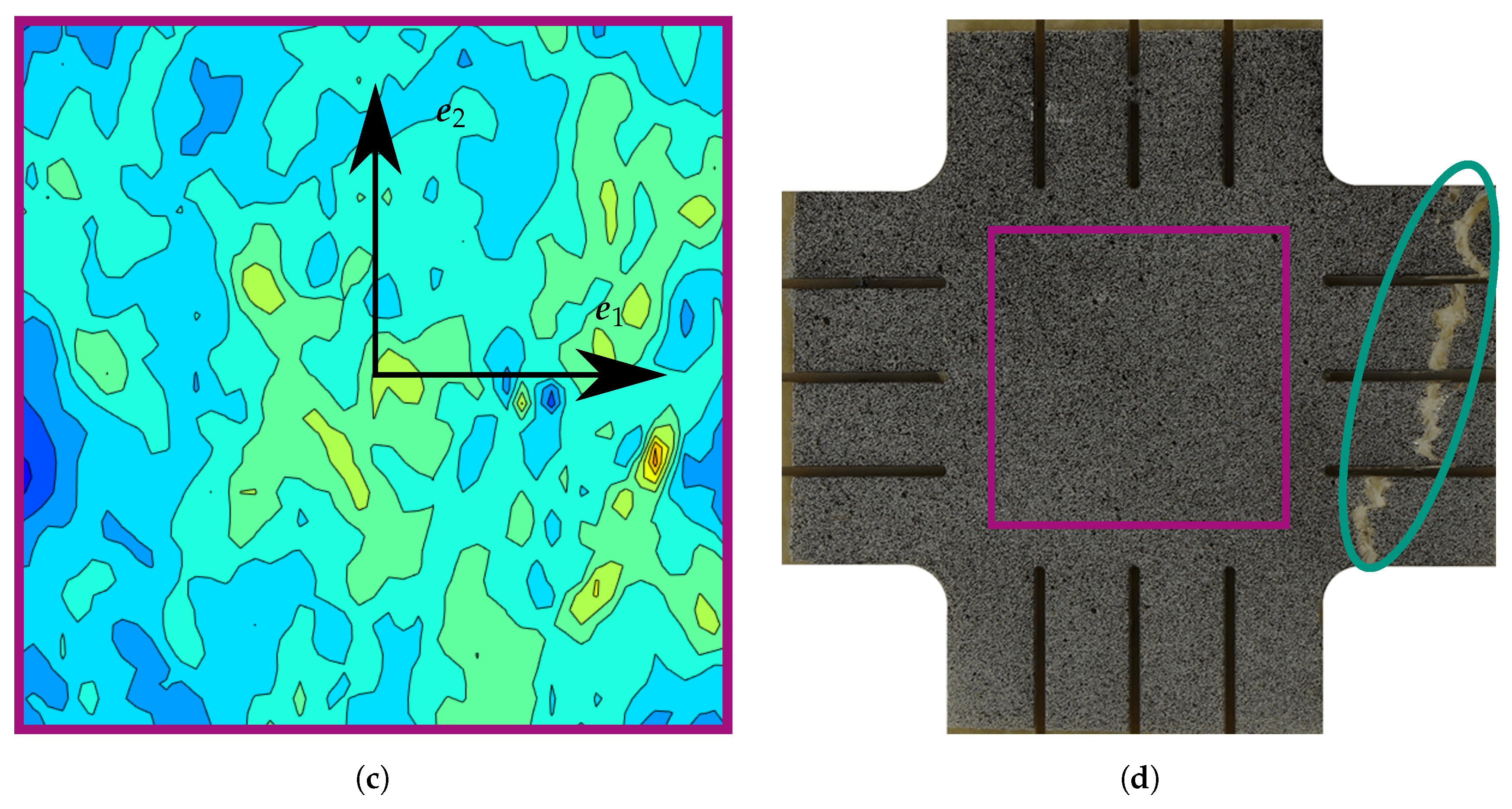
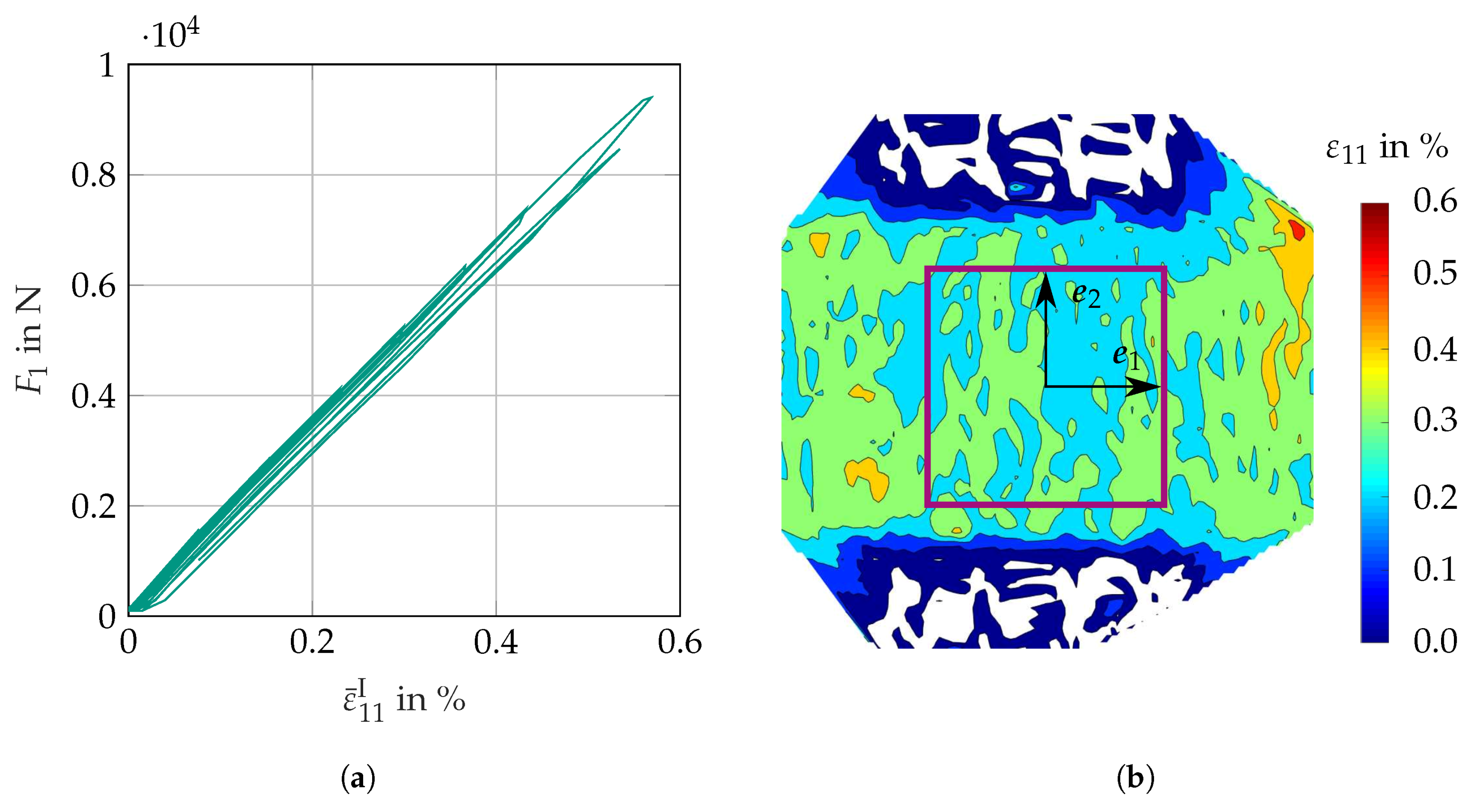
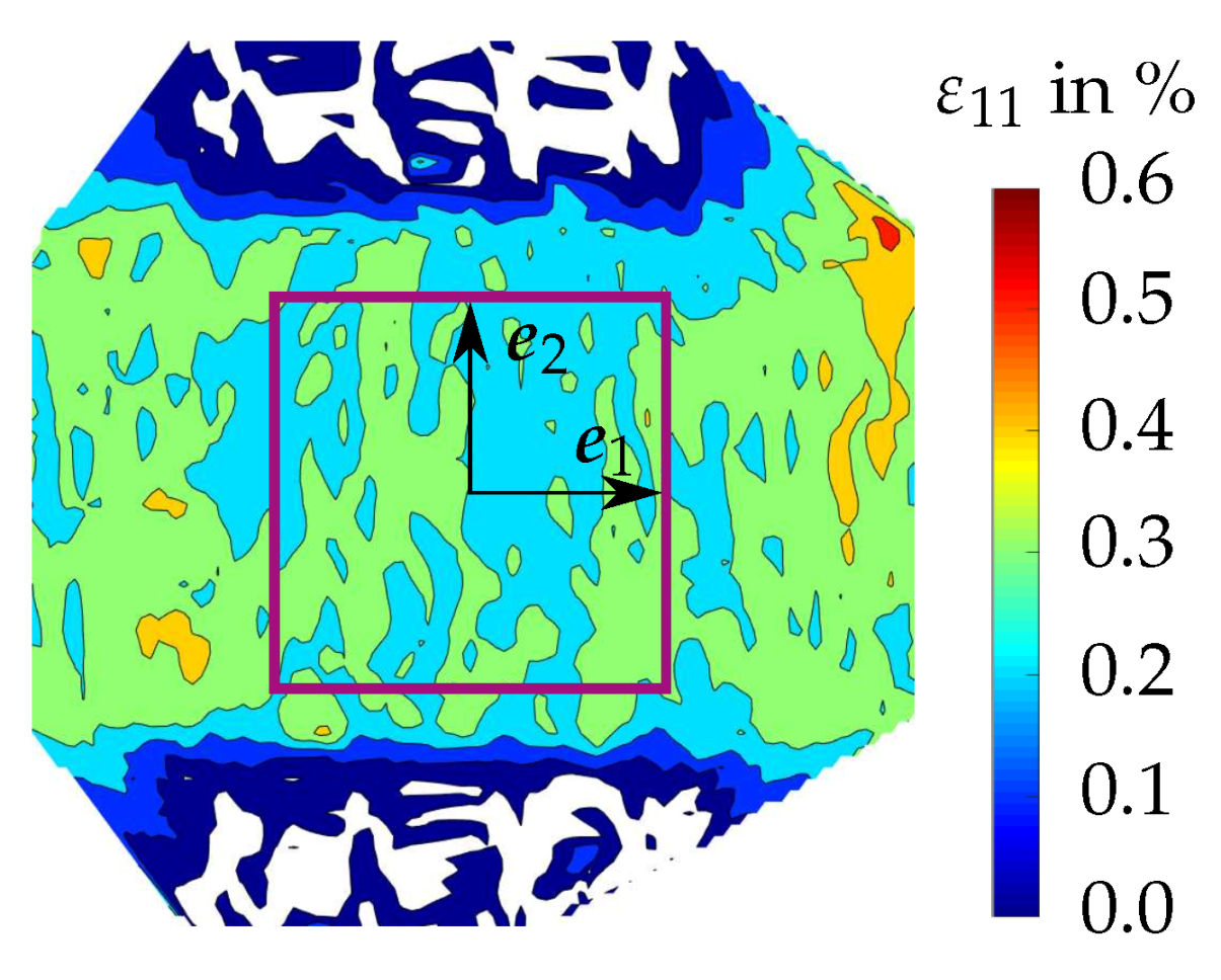
3.2. Unreinforced Specimen Arms

3.2.1. Specimen Design

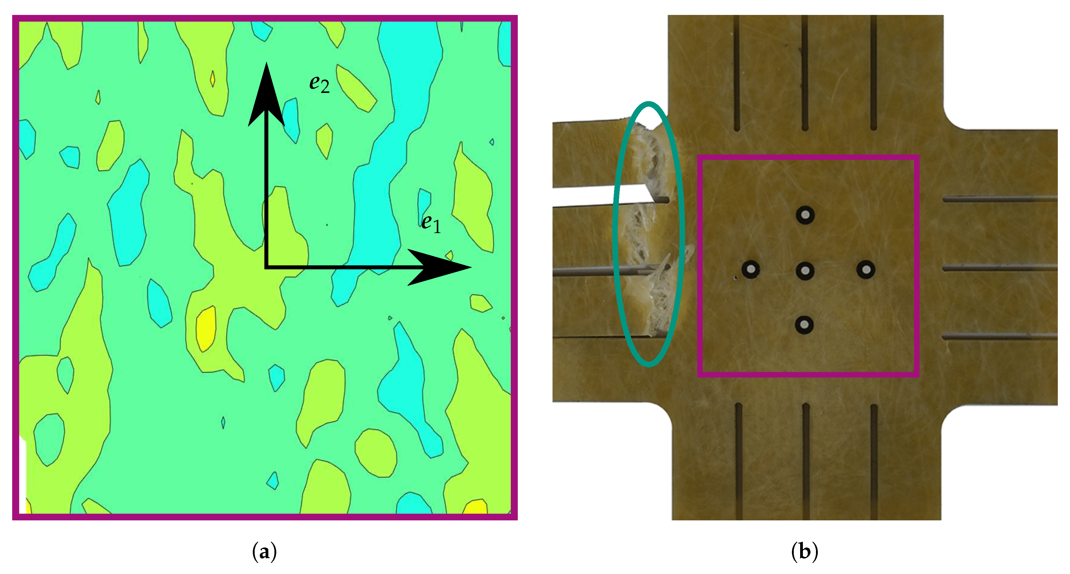
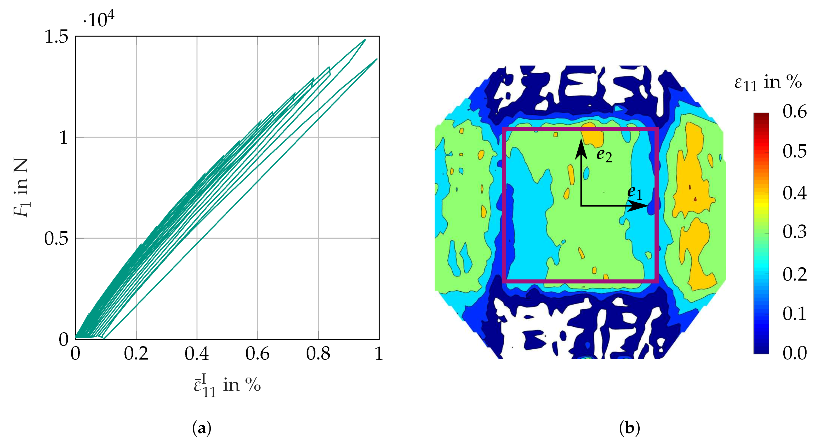
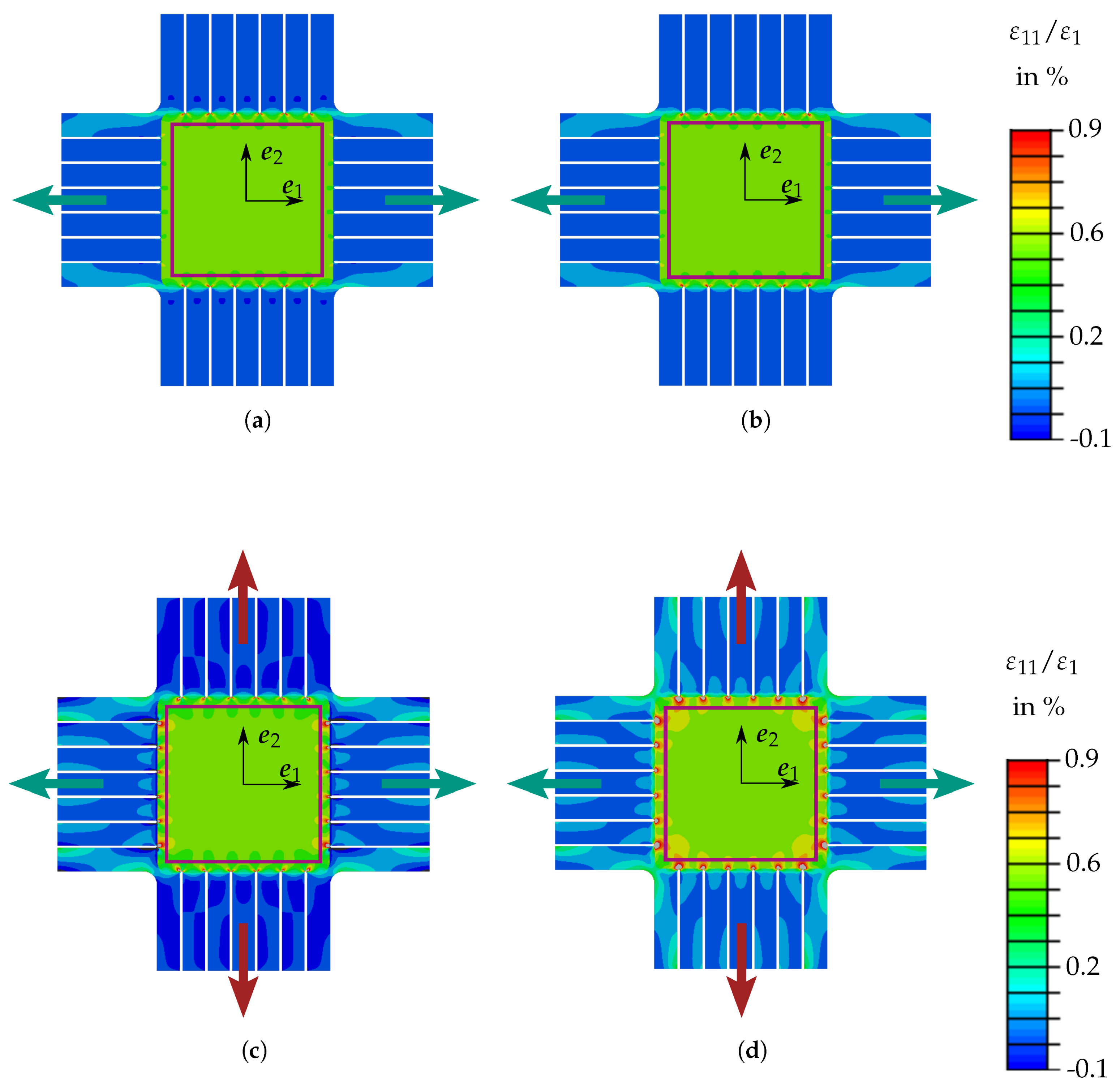
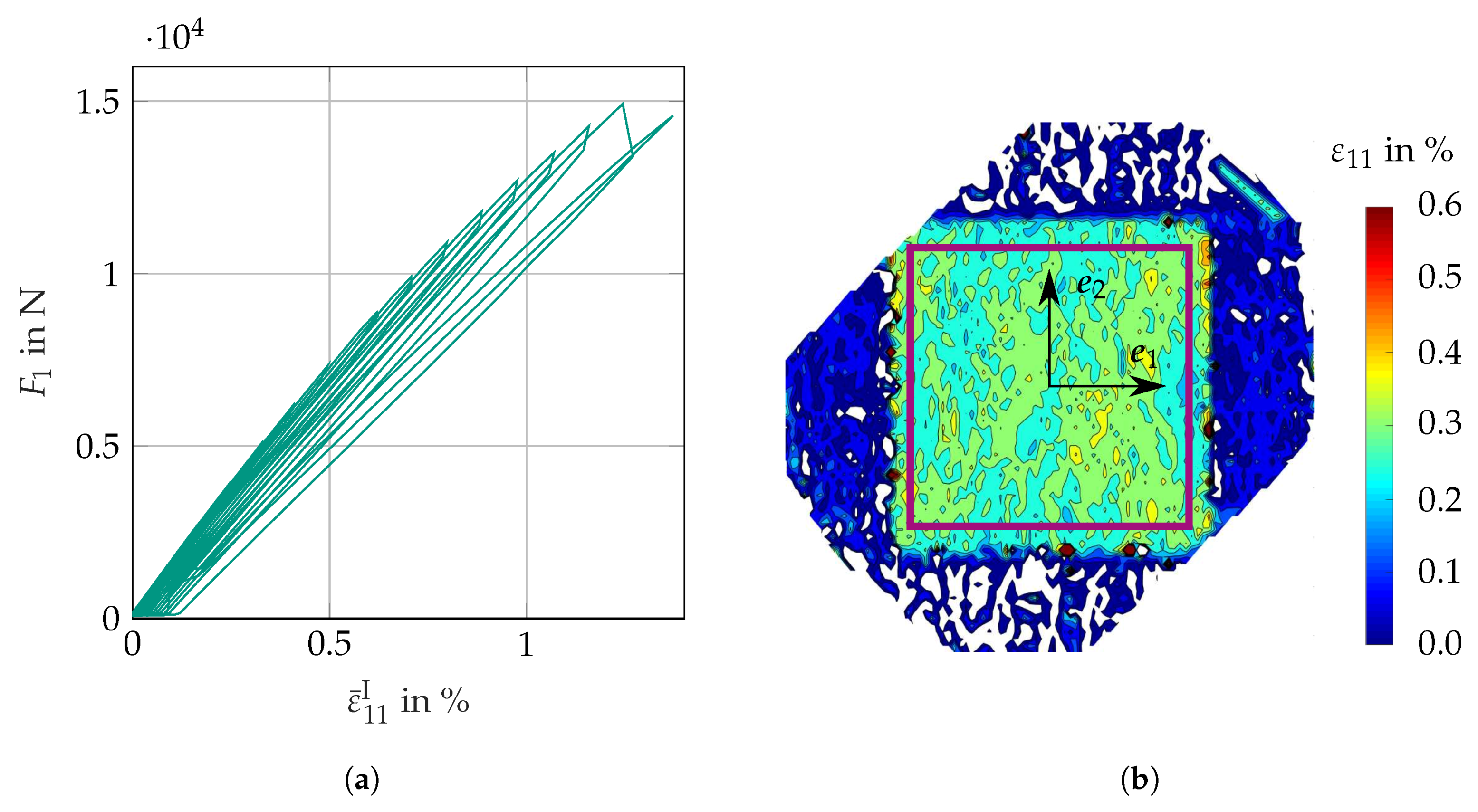
We introduce the first specimen design in line with the ISO 16842 norm [10] for biaxial tensile testing of sheet metals. Typical metals analyzed in biaxial tensile testing are aluminum and deep-drawing steels. These materials show, in contrast to SMC, large strain in the nonlinear (plastic) regime as well as work hardening. Figure 4 shows the corresponding design of a subsequently tested SMC specimen. The main advantages of water jet cutting include excellent heat removal and a minimum slit width of $1.2\mathrm{mm}$. Aiming at a maximum surface area in the arms, we decided to introduce only three slits, which lead to a reduction of the arm surface area of $7.2\%$. In contrast to the normed design, we chose the slits to extend along the entire arms, in order to avoid a damaged area enforced by the starting points of water jet cutting.

3.2.2. Results

For both the testing procedure $P_{\Gamma =0}$ and the testing procedure $P_{\Gamma =1}$, the specimens failed in the arms before a sufficiently high strain in the area of interest could be reached. Figure 5a shows the force over the strain in the $e_1$-direction for testing procedure $P_{\Gamma =0}$. The corresponding contour plot (see Figure 5b) shows that the strain in the arms is approximately equal to the strain in the area of interest, which violates optimality criterion 2. Figure 6a shows the mean values of the forces and the strains in the $e_1$-direction and the $e_2$-direction for testing procedure $P_{\Gamma =1}$. The contour plot (Figure 6b) shows that the normal strain ${\epsilon }_{11}$ is significantly higher in the arms than in the area of interest. The plot only shows the areas of positive strains. The asymmetry of the image section is due to the recording area of the cameras. A contour plot of the area of interest at the instant shortly before failure and an image of the failed specimen for all specimen designs can be found in Appendix A.

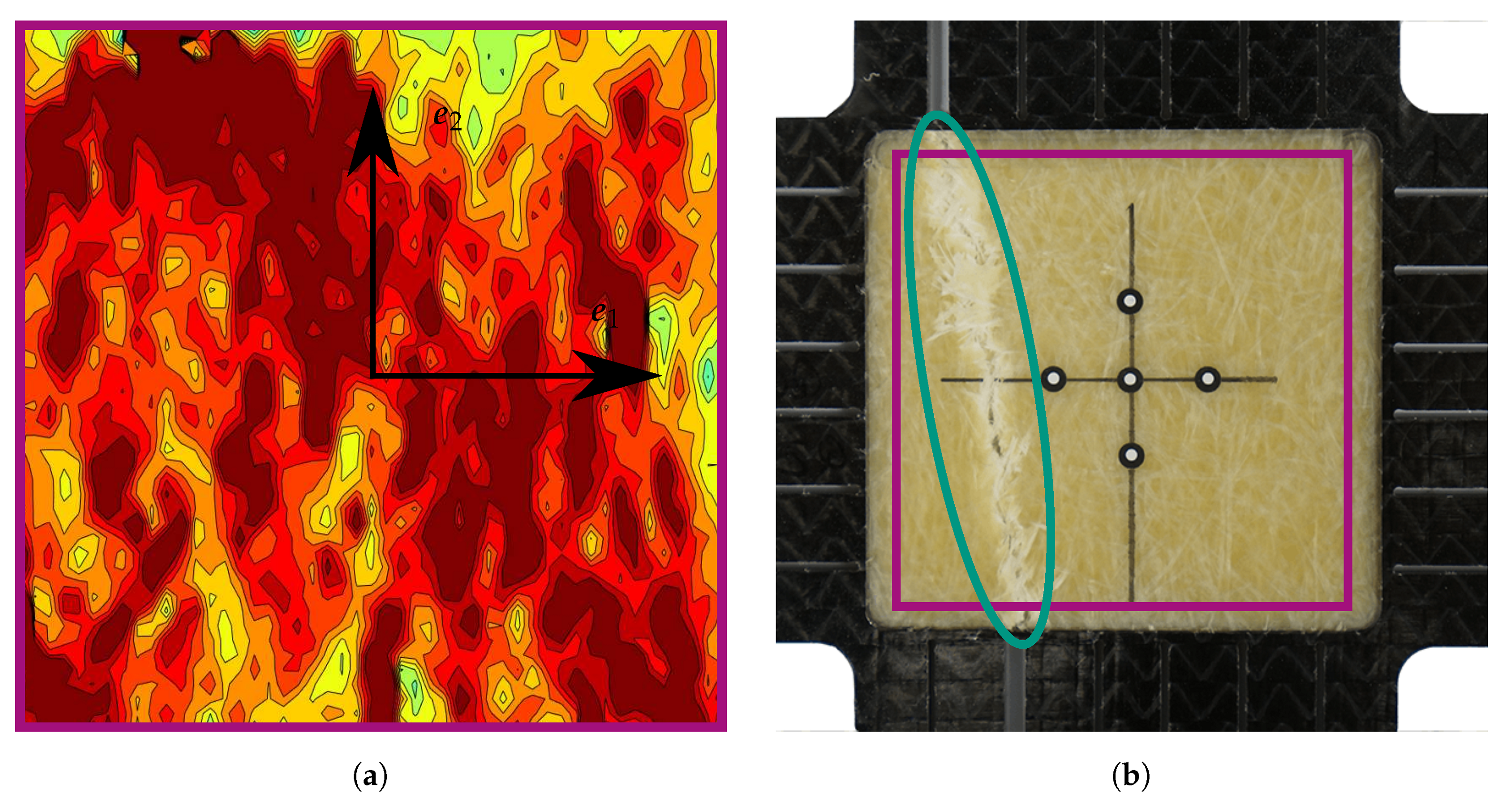
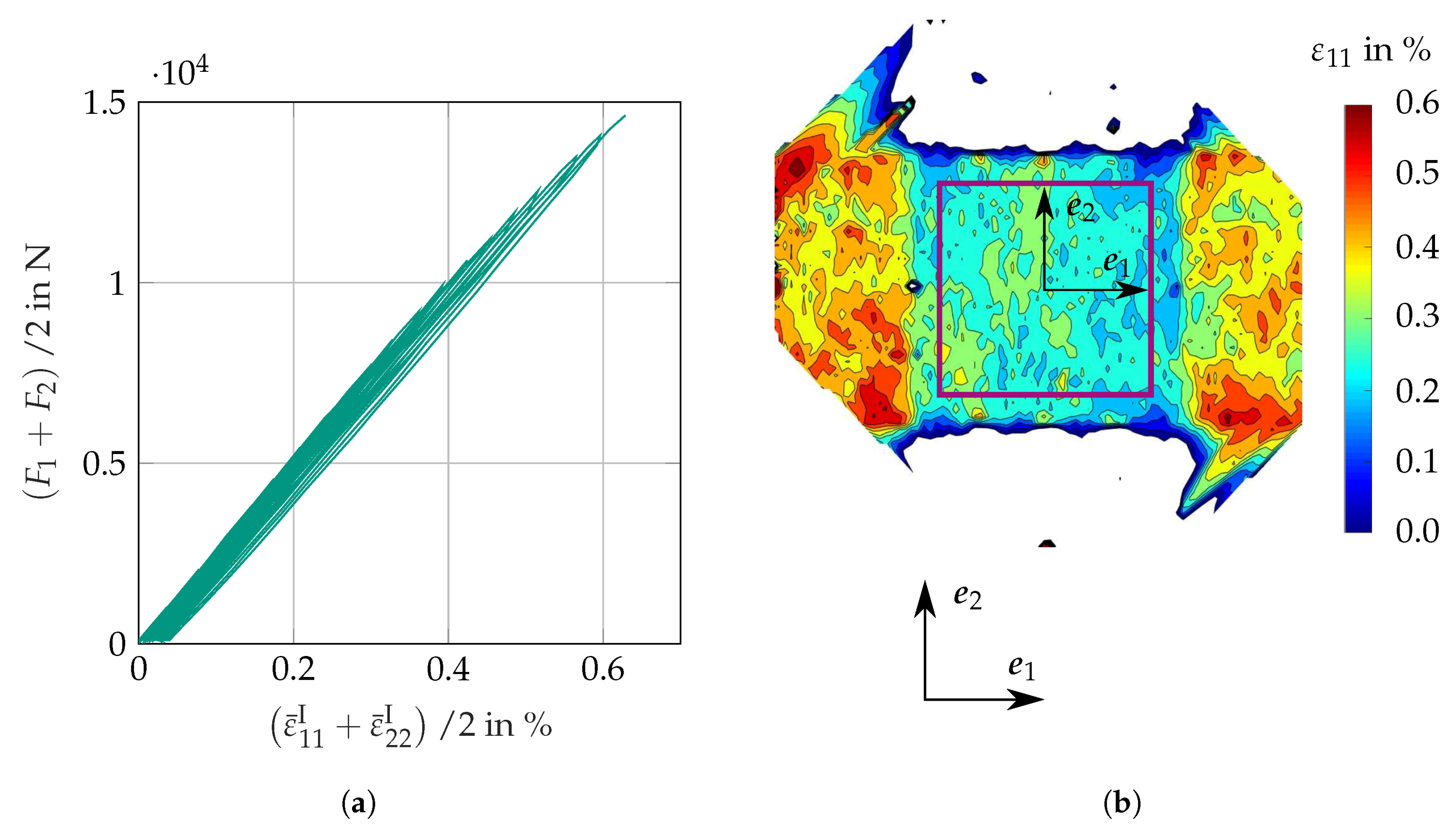
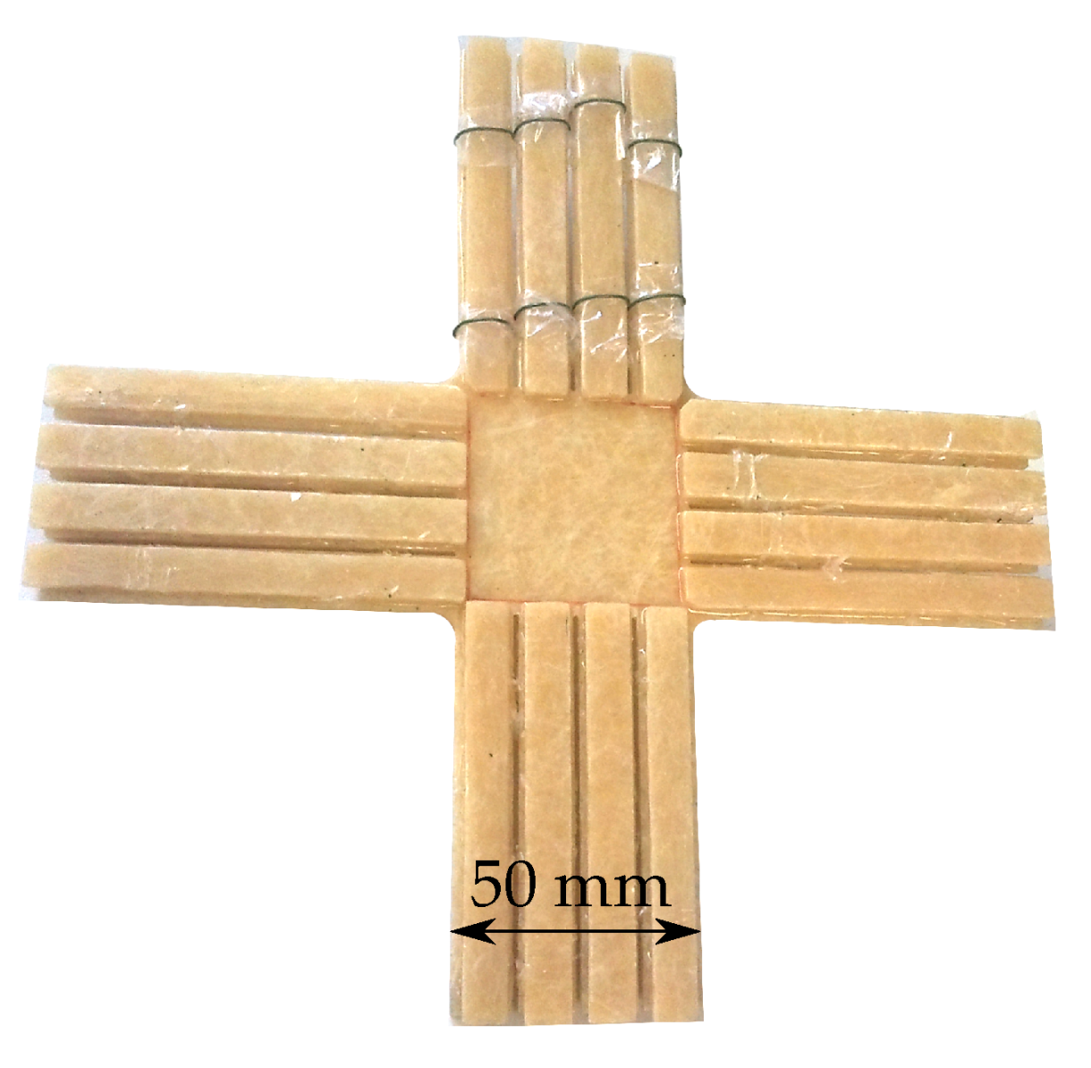
3.3. Bonded Reinforcements on the Arms

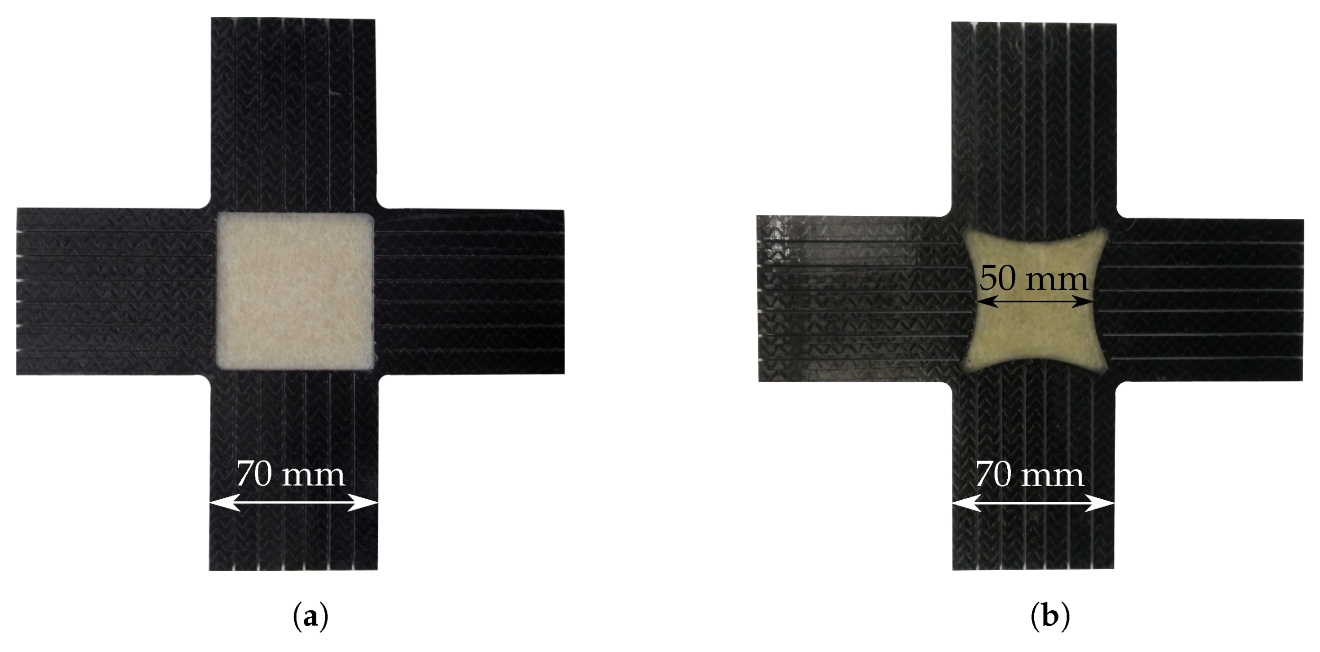
3.3.1. Specimen Design

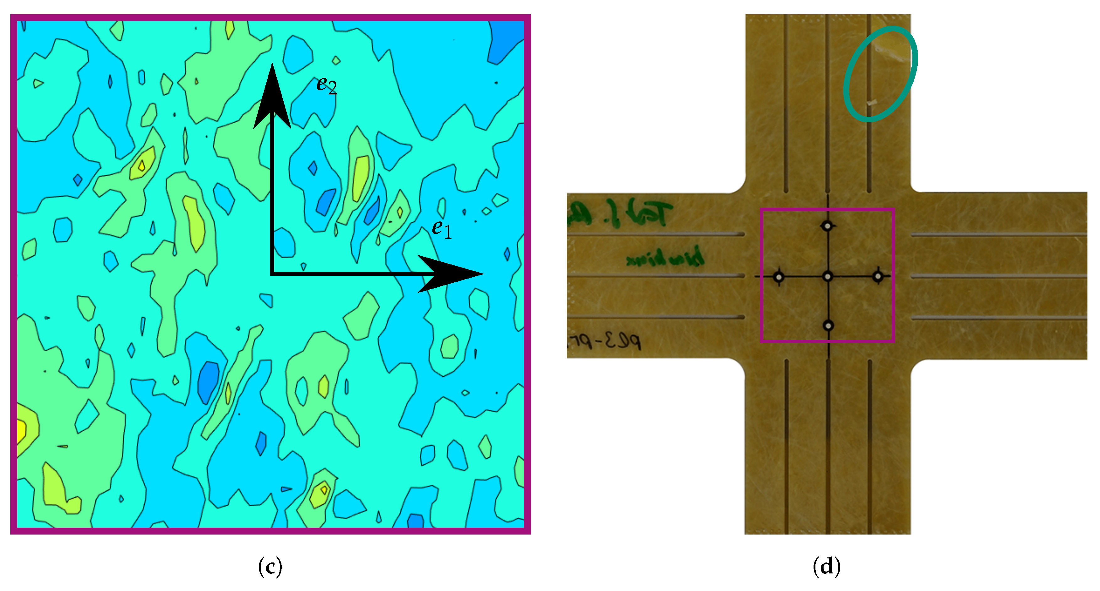
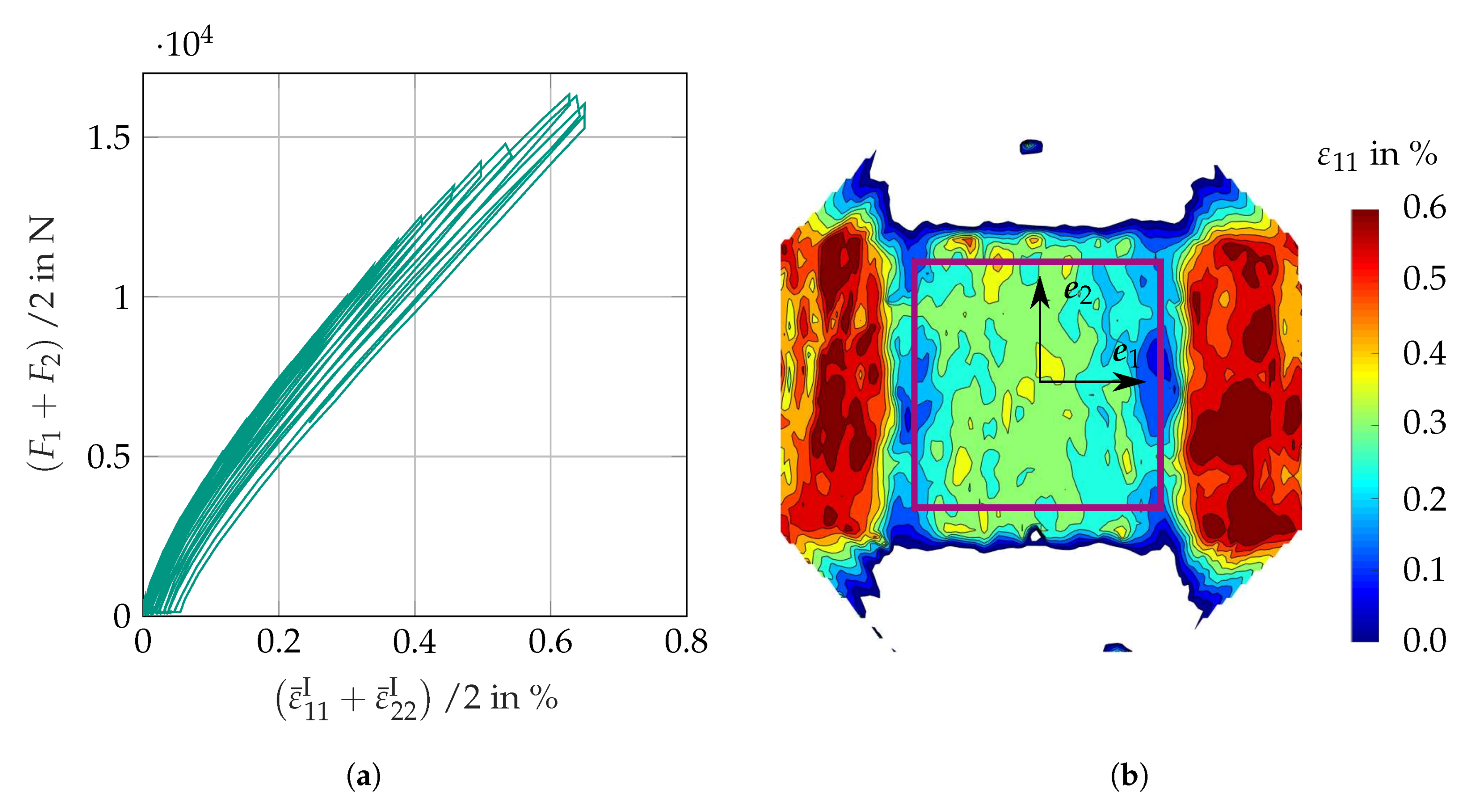
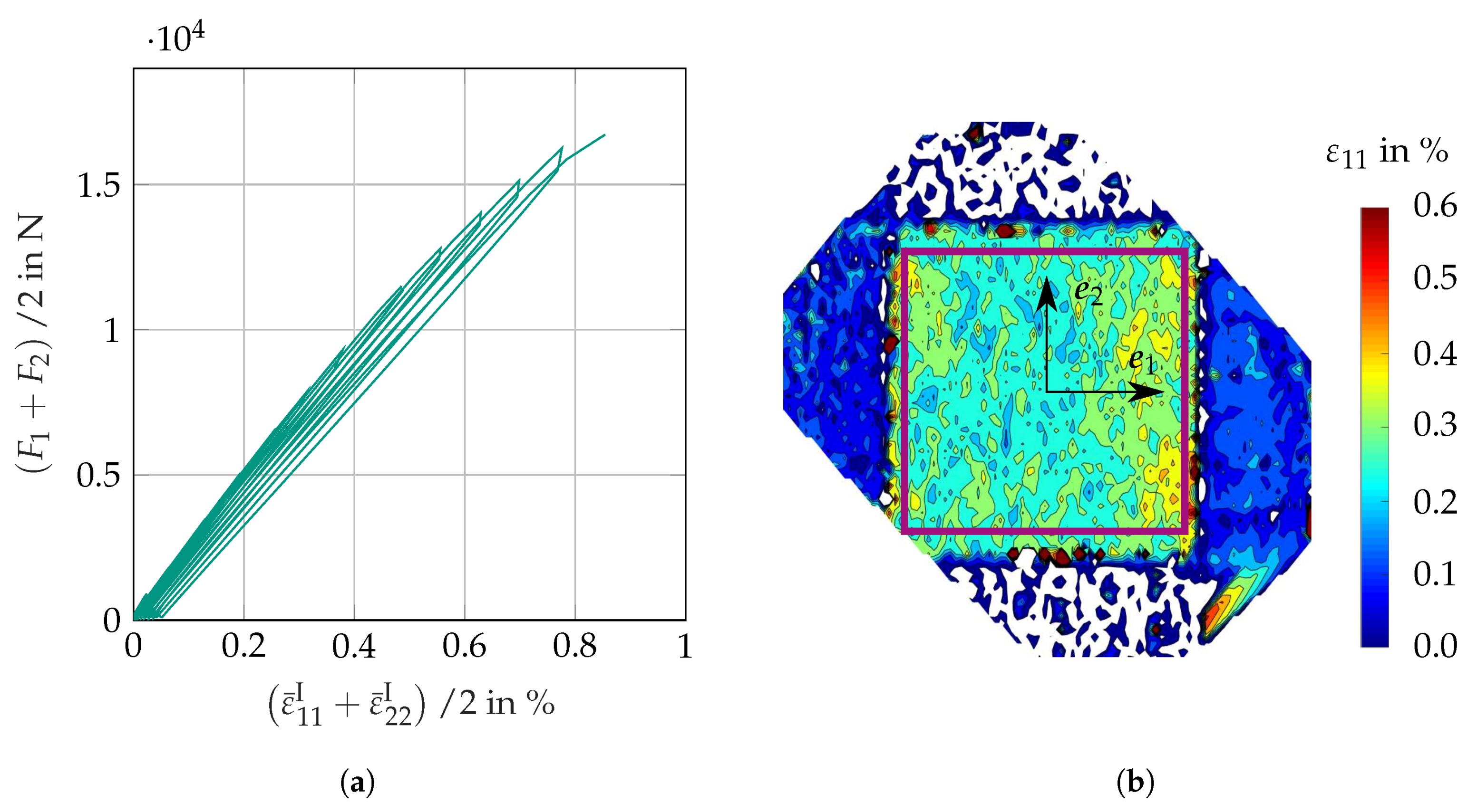
To avoid premature failure in the arms, we reinforced the specimen by bonding strips on the arms as shown in Figure 7. The upper part of the picture shows the fixation of the reinforcing strips during the manufacturing process. The strips are cut from the same SMC plate as the specimen. We glued with epoxy adhesive, which has similar material properties as the resin material (UPPH). The preparation of the specimens requires many hours of manual work and, therefore, violates optimality criterion 6.

3.3.2. Results

The bonded reinforcements significantly increase the maximum achievable strain. Here, the specimens also failed in the arms; however, a higher strain in $A^{\mathrm{I}}$ can be reached compared to the unreinforced specimen. One reason for the premature failure in the arms was a partial detachment of the bonded reinforcing strips. The force strain diagram (see Figure 8a) demonstrates the increase of the maximum reachable strain for testing procedure $P_{\Gamma =0}$. Besides that, a stiffness degradation is already visible from the decrease of the slope of the force strain curve after each cycle. However, the contour plot (Figure 8b) shows that the strain in the arms is still approximately equal to the strain in the area of interest. Figure 9a shows the mean values of the forces and the strains in the $e_1$-direction and the $e_2$-direction for the testing procedure $P_{\Gamma =1}$. Here too the maximum strain is slightly higher compared to the unreinforced specimen. The contour plot (Figure 9b) shows that the normal strain in the arms is still significantly higher than the normal strain in the area of interest.

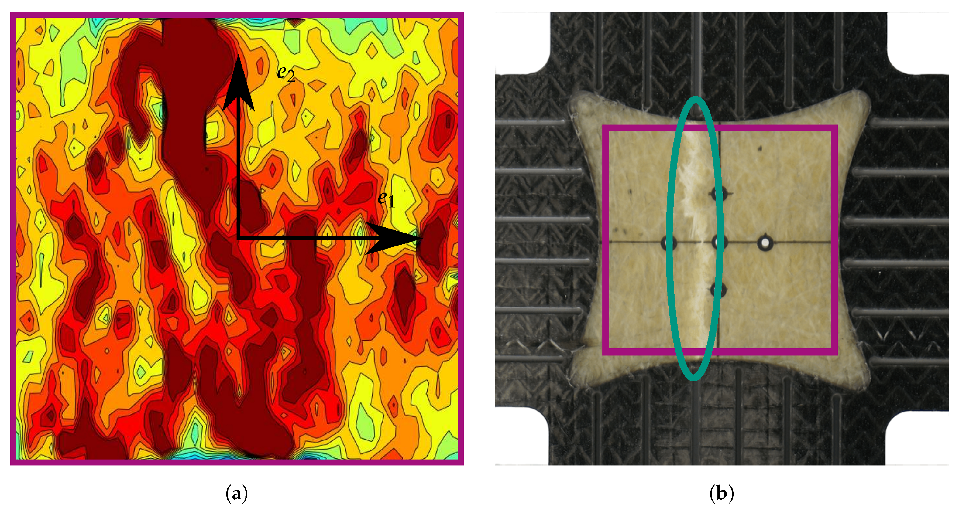
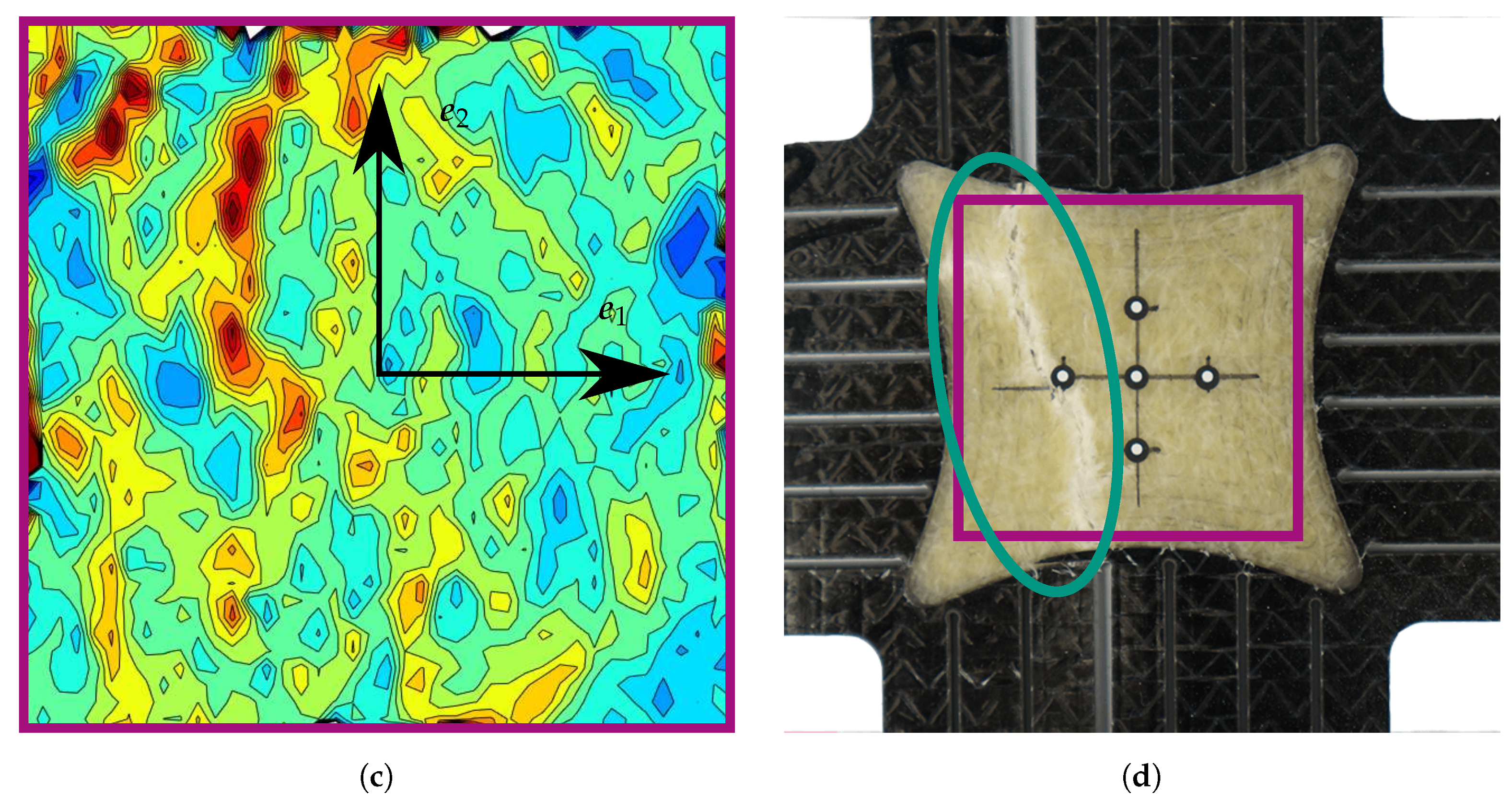
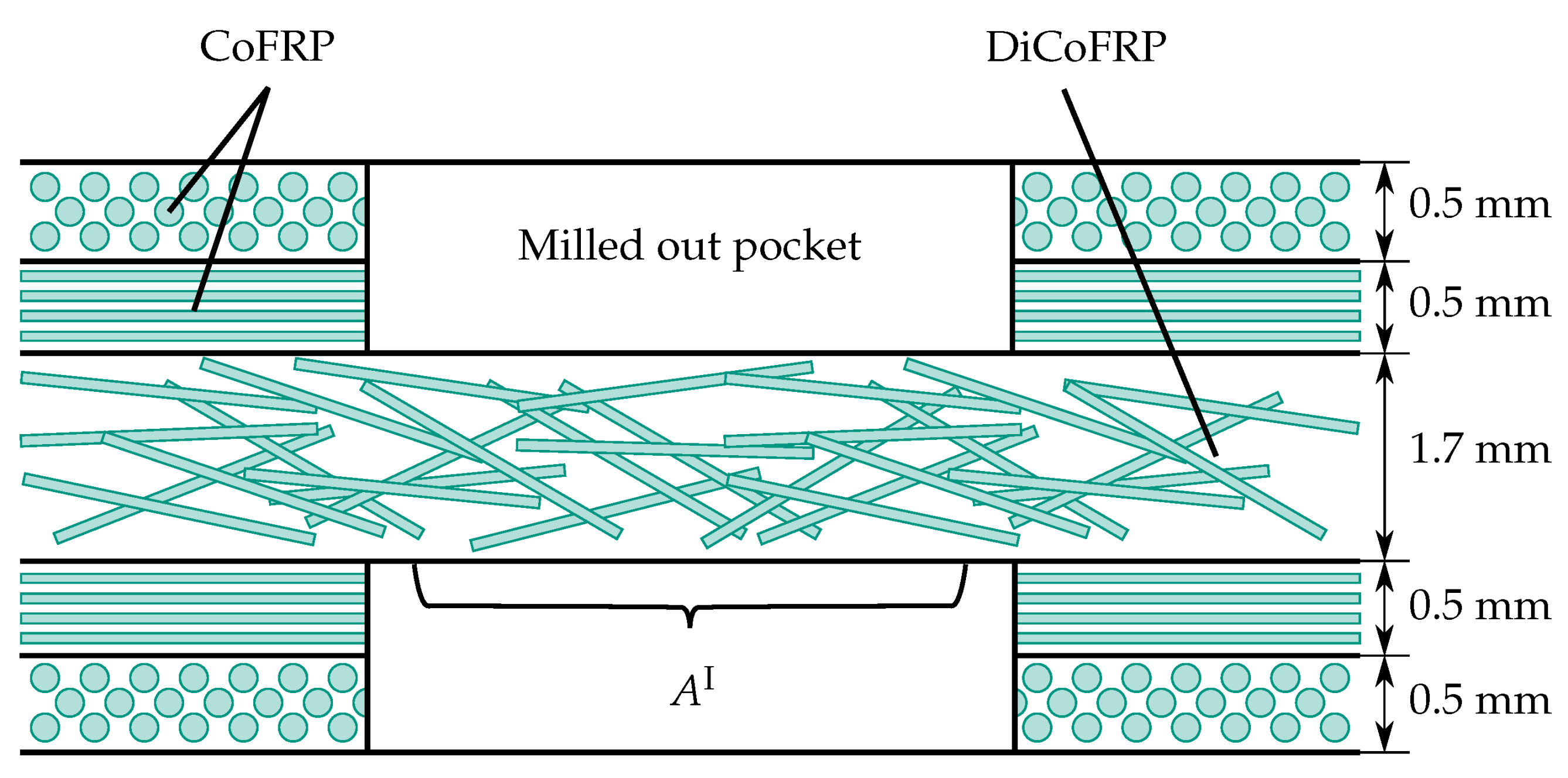
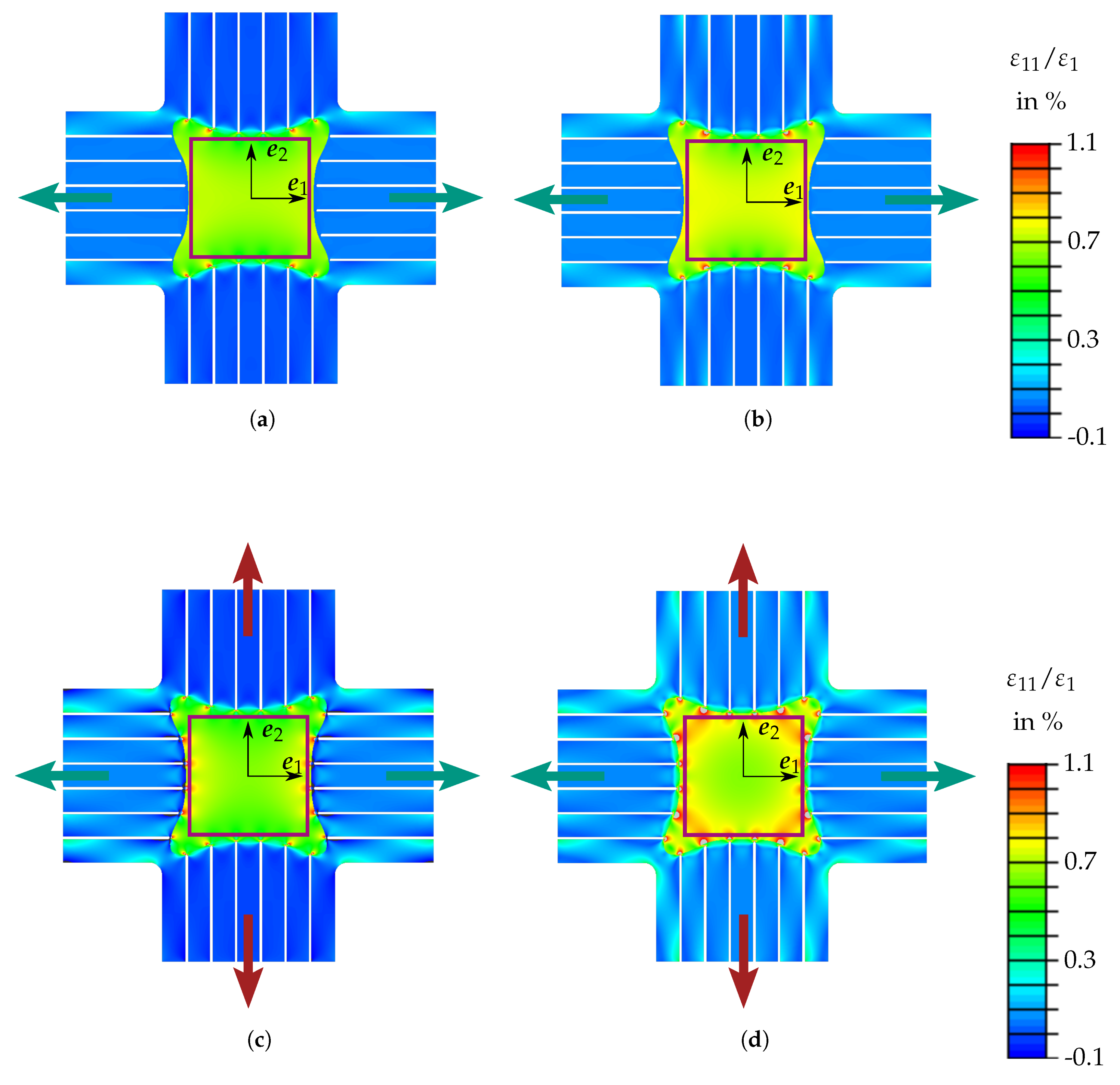
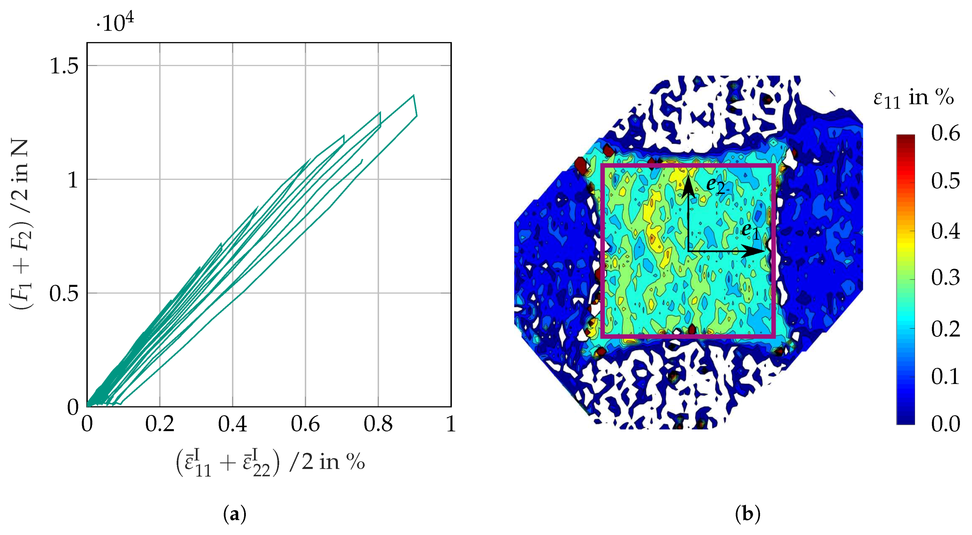
3.4. Continuous Fiber Reinforced Arms

3.4.1. Particularities in Specimen Manufacturing

To overcome the disadvantages of bonded reinforcements on the arms, we considered the manufacturing process of SMC with unidirectional tapes [27]. The unidirectional tapes’ constituents are UPPH resin (also in SMC) and $60\mathrm{vol}\%$ carbon fibers. The plates were manufactured with $100\%$ mold coverage to avoid in-mold slip of the layers during the compression molding. More details regarding the co-molding process can be found in [28]. Figure 10 shows the symmetric layup, where the middle layer consists of SMC and the outer layers are tapes with a fiber orientation perpendicular to each other.

Figure 10 and Figure 11 depict the pockets machined into the continuous layers of the specimen. The milling process of these pockets is described in the following.

For this process, a diamond coated end mill with eight cutting edges and a multi-cut geometry by Hufschmied GmbH (Bobingen, Germany) was used. The specimens were clamped into position with a line clamping on two sides of the pocket as to minimize the distance of the pocket center to either side of the clamping. This clamping strategy also allowed for a continuous process, i.e., no reclamping was necessary. We generated the tool path from a computer-aided design (CAD) model of the specimens with the Siemens NX computer-aided manufacturing (CAM) system. The values of the cutting speed $v_{\mathrm{c}}$ and the feed per tooth $f_{\mathrm{PT}}$ were experimentally qualified during preliminary tests with a similar material and the same tool. These parameters were set at $v_{\mathrm{c}}=66\mathrm{m}/\min$ and $f_{\mathrm{PT}}=0.07\mathrm{mm}$, respectively. The main challenges in machining of the pockets were to prevent any kind of delamination, which is critical in plunging into the material, and to obtain a smooth, even surface without heat-induced damages or altered material properties. After the first cut with a depth of $1\mathrm{mm}$, in some areas of the pocket, remnants of the continuous fibers were found. These remnants likely originate from a movement of the unidirectional tapes in $e_3$-direction during the compression molding process. Nevertheless, further machining steps were performed in $0.1\mathrm{mm}$ steps to ensure a pure SMC sector in the area of interest.

3.4.2. Specimen Design

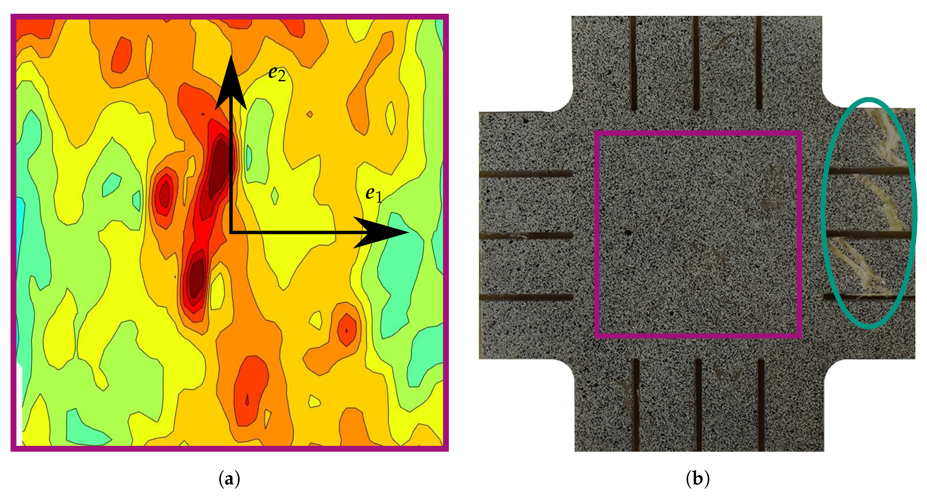
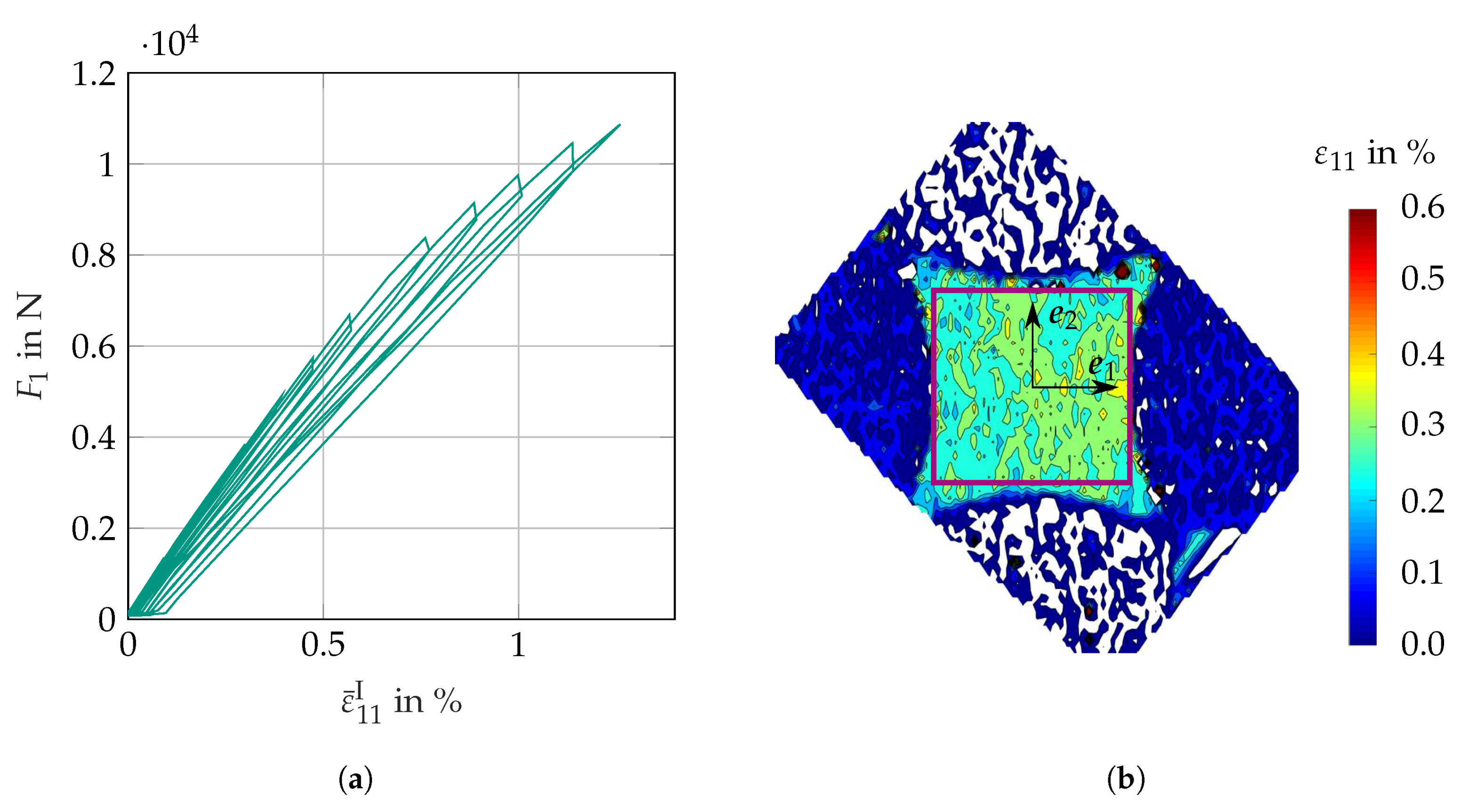
The novel manufacturing technique significantly increases the arms’ stiffness and strength in the loading directions and, therefore, defines new constraints in the search for the optimal geometry. Here, we introduce two geometries that we consider to be a good compromise between the optimality criteria presented in Section 3.1. As there are difficulties in parametric shape optimization [29], we decided to perform a high number (thousands) of FE (finite element) simulations and thoroughly selected suitable solutions manually.

The first geometry, in the following called geometry 1, follows the design of the unreinforced specimen. Figure 11a shows an image of the design. The significant increase of arm strength allowed for incorporating six slits in each arm to reduce the peak stress at the slit’s ends and reduce load transition in the slits perpendicular to the normal stress direction. The slits end slightly before the beginning of the milled out pockets.

Figure 12 depicts strain fields computed from finite element simulations on geometry 1. We took advantage of the specimen’s symmetry and only simulated one fourth of the geometry with a fine discretization of shell elements. As we were only interested in trends of different geometry modifications and not precise strain fields, we assumed linear elastic isotropic material behavior with a different stiffness and element thickness in the pocket and the reinforced area. We would like to remark here that a precise quantitative comparison of designs should include the prediction of macroscopic cracks leading to macroscopic failure and an evaluation of the observability of the damage stage. This was not achievable within the scope of the presented research. The upper images show the strain distributions for a uniaxial loading scenario $P_{\Gamma =0}$ in the horizontal $e_1$-direction. The strain distribution in the area of interest shows only small fluctuations. The outer arms contribute more to the load transition into the specimen, as part of the outer load is transmitted into the tape-reinforced regions. The lower images visualize the strain distribution for an equi-biaxial tensile loading scenario $P_{\Gamma =1}$. The distribution of the normal strain ${\epsilon }_{11}$ (Figure 12c) shows peaks at the end of the horizontal slits. Figure 12d depicts the distribution of the maximal principal strain ${\epsilon }_1$. Due to the reduced stiffness in the area of interest, here, the strain is significantly higher than in the earlier discussed designs.

Geometry 2 is different from geometry 1 in such a way that the milled out area has curved edges (see Figure 11). In analogy to uniaxial tapered bone specimens, our aim was to achieve an elevated stress level in the area of interest. Figure 13 shows the strain fields for uniaxial and biaxial load. For the uniaxial loading case, the stress distribution is more homogeneous; however, in front of the second outer slit end, there is a significant strain concentration. For the case of equi-biaxial loading, the strain concentrations, especially the principal strain ${\epsilon }_1$ (see Figure 13d), shows significant peaks towards the end of the slits.

3.4.3. Results

The contour plots in Figure 14, Figure 15, Figure 16 and Figure 17 show that the experimental strain distributions are similar to those predicted from the simulations. Figure 14b confirms the relatively homogeneous strain field of Figure 12a for geometry 1 and testing procedure $P_{\Gamma =0}$. For testing procedure $P_{\Gamma =1}$, the small strain peaks at the end of the slits mentioned in conjunction with Figure 12c are visible again (see Figure 15b). For both testing procedures, the strain in the area of interest is significantly higher than the strain in the arms. Failure occurs in the area of interest when a sufficiently high strain is reached. Figure 14a shows the force over the strain in the $e_1$-direction for the testing procedure $P_{\Gamma =0}$. This figure demonstrates that the continuous fiber reinforced layers significantly increase the maximum achievable strain. A stiffness degradation is clearly visible. Figure 15a shows that the reinforcement increases the maximum achievable strain also for testing procedure $P_{\Gamma =1}$.

Figure 16b and Figure 17b show the contour plots of geometry 2. Here too, the strain in the area of interest is significantly higher than in the arms. The strain peaks at the end of the slits, as mentioned for Figure 13, are visible, particularly pronounced for testing procedure $P_{\Gamma =1}$. Failure occcurs in the area of interest, but is initiated at the end of the slits. The force strain diagrams (Figure 16a and Figure 17a) show that also geometry 2 increases the maximum achievable strain, but slightly less than geometry 1.

4. Discussion

Table 2. Maximum attained strain within one experiment for the different biaxial specimen designs and, for reference, the failure strain of a uniaxial bone specimen. Here, the operator $max\left(·\right)$ denotes the maximum value in the course of the experiment.

Reinforcement Type		None	Bonded SMC	Cont. Geom. 1	Cont. Geom. 2	Uniax. Bone
$max\left({\overline{\epsilon }}_{11}^{\mathrm{I}}\right)$	$P_{\Gamma =0}$	0.57%	1.00%	1.37%	1.26%	1.57%
$max\left({\overline{\epsilon }}_{11}^{\mathrm{I}}+{\overline{\epsilon }}_{22}^{\mathrm{I}}\right)/2$	$P_{\Gamma =1}$	0.63%	0.65%	0.85%	0.76%	-

summarizes the maximum attained normal strains averaged over the area of interest $max\left({\overline{\epsilon }}_{11}^{\mathrm{I}}\right)$ in loading scenario $P_{\Gamma =0}$ and $max\left({\overline{\epsilon }}_{11}^{\mathrm{I}}+{\overline{\epsilon }}_{22}^{\mathrm{I}}\right)/2$ in loading scenario $P_{\Gamma =1}$ accordingly. These strains especially quantify the level of achievable strain in the area of interest and thus allow for evaluating the specimen with regard to criterion 2, since damage only occurs if sufficiently high strains are achieved (criterion 2 of the previously defined specimen requirements (Section 3.1)). The ranking of the specimens is equal for both loading scenarios. The unreinforced specimen fails at the lowest strains, bonded reinforcements on the arms lead to a significant improvement, the continuous fiber reinforced specimens perform better, whereas geometry 1 performs slightly better than geometry 2. In loading scenario $P_{\Gamma =0}$, the continuous reinforced geometry 1 reaches $87\%$ of the failure strain measured in a uniaxial tensile bone specimen tested on the same machine. In parallel to the maximum strain reached in the area of interest, a steady reduction of the slope in the force–strain plots indicates the evolution of damage. A visual comparison of these plots indicates a good agreement with Table 2, such that the specimens that allow for the observation of higher strains also show a higher slope reduction in the force–strain plot. The interpretation of the results requires great caution, since only one experiment per specimen geometry and load case was performed.

Geometry 1 also performs equal or superior to the other specimens considering optimality criteria 1 and 3. Force $F_1$ is almost ideally transferred via a homogeneous normal stress in the $e_1$-direction, force $F_2$ governs the normal stress in the $e_2$-direction accordingly. Therefore, by a variation of the loading ratio $\Gamma$, we can achieve any planar tensile stress ratio. The strain state in the area of interest is rather homogeneous because of the high number of slits, that reduce the strain, as shown by DIC and FE simulations. Consequently, we may assume that (due to the slits) the disturbing effect of the arms on the stress distribution is weak and the stress field is likewise approximately homogeneous so that the stress state can be estimated from the forces divided by the material cross section in the area of interest. The thus obtained material parameters provide an estimate of the material behavior and can serve as a starting value for an inverse parameter identification (partly criterion 4).

When comparing geometry 1 and geometry 2 of the continuous fiber reinforced specimen, geometry 1 also shows advantages concerning the larger size of the area of interest (criterion 5). The manufacturing effort (criterion 6) is the lowest in the unreinforced specimen. The bonded specimen requires a large amount of manual work. The continuous fiber reinforced specimen preparation requires an additional manufacturing technique (milling), but is more time-efficient compared to the bonded specimen.

One experiment per design and load scenario is, of course, not statistically representative. We admit that our experimental investigation with only one specimen may not provide a precise quantitative design estimate; however, the experiments are (i) plausible within each experiment and in comparison of all experiments, and (ii) show a good agreement with the FE simulations (continuous fiber reinforced specimen). The experiments in this work, hence, provide a preliminary estimation of the specimens’ suitability.

5. Conclusions

This work provided experimental as well as numerical results to support the selection of a suitable specimen design for the characterization of the damage behavior of SMC. The authors, however, did not aim to characterize the anisotropic damage behavior of SMC, as the number of experiments was significantly too low and the differentiation of damage, viscoelasticity, and plasticity in discontinuous fiber reinforced polymers [30] along with their parameter identification are still not fully understood. One result could be an understanding of the anisotropic stress–strain behavior of SMC. Geometry 1 of the continuous fiber reinforced specimen performed superior for our application, i.e., the optimality criteria and their prioritization we aimed for. The main advantages are the highest achievable strain in the area of interest among all specimen, the homogeneity of the strain in the area of interest, the large area of interest, and a moderate manufacturing effort.

References

1. Ohtake, Y.; Rokugawa, S.; Masumoto, H. Geometry determination of cruciform-type specimen and biaxial tensile test of C/C composites. Key Eng. Mater. 1999, 164–165, 151–154. [Google Scholar] [CrossRef]
2. Deng, N.; Kuwabara, T.; Korkolis, Y.P. Cruciform specimen design and verification for constitutive identification of anisotropic sheets. Exp. Mech. 2015, 55, 1005–1022. [Google Scholar] [CrossRef]
3. Kuwabara, T.; Ikeda, S.; Kuroda, K. Measurement and analysis of differential work hardening in cold-rolled steel sheet under biaxial tension. J. Mater. Process. Technol. 1998, 80–81, 517–523. [Google Scholar] [CrossRef]
4. Makinde, A.; Thibodeau, L.; Neale, K.W. Development of an apparatus for biaxial testing using cruciform specimens. Exp. Mech. 1992, 32, 138–144. [Google Scholar] [CrossRef]
5. Demmerle, S.; Boehler, J.P. Optimal design of biaxial tensile cruciform specimens. J. Mech. Phys. Solids 1993, 41, 143–181. [Google Scholar] [CrossRef]
6. Kelly, D.A. Problems in creep testing under biaxial stress systems. J. Strain Anal. 1976, 11, 1–6. [Google Scholar] [CrossRef]
7. Boehler, J.P.; Demmerle, S.; Koss, S. A new direct biaxial testing machine for anisotropic materials. Exp. Mech. 1994, 34, 1–9. [Google Scholar] [CrossRef]
8. Hoferlin, E.; Van Bael, A.; Van Houtte, P.; Steyaert, G.; De Maré, C. Design of a biaxial tensile test and its use for the validation of crystallographic yield loci. Model. Simul. Mater. Sci. Eng. 2000, 8, 423–433. [Google Scholar] [CrossRef]
9. Hannon, A.; Tiernan, P. A review of planar biaxial tensile test systems for sheet metal. J. Mater. Process. Technol. 2008, 198, 1–13. [Google Scholar] [CrossRef]
10. International Organization for Standardization. Metallic Materials—Sheet and Strip—Biaxial Tensile Testing Method Using a Cruciform Test Piece; ISO 16842; International Organization for Standardization: Geneva, Switzerland, 2014. [Google Scholar]
11. Green, D.E.; Neale, K.W.; MacEwen, S.R.; Makinde, A.; Perrin, R. Experimental investigation of the biaxial behaviour of an aluminum sheet. Int. J. Plast. 2004, 20, 1677–1706. [Google Scholar] [CrossRef]
12. Smits, A.; Van Hemelrijck, D.; Philippidis, T.P.; Cardon, A. Design of a cruciform specimen for biaxial testing of fibre reinforced composite laminates. Compos. Sci. Technol. 2006, 66, 964–975. [Google Scholar] [CrossRef]
13. Van Hemelrijck, D.; Ramault, C.; Markis, A.; Clarke, A.R.; Williamson, C.; Gower, M.; Shaw, R.; Mera, R.; Lamkanfi, E.; Van Paepegem, W. Biaxial testing of fibre reinforced composites. In Proceedings of the 16th International Conference on Composite Materials, Xi’an, China, 20–25 August 2007; pp. 1–8. [Google Scholar]
14. Makris, A.; Vandenbergh, T.; Ramault, C.; Van Hemelrijck, D.; Lamkanfi, E.; Van Paepegem, W. Shape optimisation of a biaxially loaded cruciform specimen. Polym. Test. 2010, 29, 216–223. [Google Scholar] [CrossRef]
15. Lamkanfi, E.; Van Paepegem, W.; Degrieck, J.; Ramault, C.; Makris, A.; Van Hemelrijck, D. Strain distribution in cruciform specimens subjected to biaxial loading conditions. Part 2: Influence of geometrical discontinuities. Polym. Test. 2010, 29, 132–138. [Google Scholar] [CrossRef]
16. Gower, M.R.L.; Shaw, R.M. Towards a planar cruciform specimen for biaxial characterisation of polymer matrix composites. Appl. Mech. Mater. 2010, 24–25, 115–120. [Google Scholar] [CrossRef]
17. Serna Moreno, M.; Martínez Vicente, J.; López Cela, J. Failure strain and stress fields of a chopped glass-reinforced polyester under biaxial loading. Compos. Struct. 2013, 103, 27–33. [Google Scholar] [CrossRef]
18. Hohberg, M.; Kärger, L.; Bücheler, D.; Henning, F. Rheological In-Mold Measurements and Characterizations of Sheet-Molding-Compound (SMC) Formulations with Different Constitution Properties by Using a Compressible Shell Model. Int. Polym. Process. 2017, 32, 659–668. [Google Scholar] [CrossRef]
19. Asadi, A.; Miller, M.; Sultana, S.; Moon, R.J.; Kalaitzidou, K. Introducing cellulose nanocrystals in sheet molding compounds (SMC). Compos. Part A Appl. Sci. Manuf. 2016, 88, 206–215. [Google Scholar] [CrossRef]
20. Mahnken, R.; Stein, E. A unified approach for parameter identification of inelastic material models in the frame of the finite element method. Comput. Methods Appl. Mech. Eng. 1996, 136, 225–258. [Google Scholar] [CrossRef]
21. Mahnken, R.; Stein, E. Parameter identification for viscoplastic models based on analytical derivatives of a least-squares functional and stability investigations. Int. J. Plast. 1996, 12, 451–479. [Google Scholar] [CrossRef]
22. Cooreman, S.; Lecompte, D.; Sol, H.; Vantomme, J.; Debruyne, D. Identification of mechanical material behavior through inverse modeling and DIC. Exp. Mech. 2007, 48, 421–433. [Google Scholar] [CrossRef]
23. Lecompte, D.; Smits, A.; Sol, H.; Vantomme, J.; Van Hemelrijck, D. Mixed numerical-experimental technique for orthotropic parameter identification using biaxial tensile tests on cruciform specimens. Int. J. Solids Struct. 2007, 44, 1643–1656. [Google Scholar] [CrossRef]
24. Schemmann, M.; Brylka, B.; Müller, V.; Kehrer, L.; Böhlke, T. Mean field homogenization of discontinous fiber reinforced polymers and parameter identification of biaxial tensile tests through inverse modeling. In Proceedings of the 20th International Conference on Composite Materials, Copenhagen, Denmark, 19–24 July 2015. [Google Scholar]
25. Schemmann, M.; Gajek, S.; Böhlke, T. Biaxial tensile tests and microstructure-based inverse parameter identification of inhomogeneous SMC composites. In Advances in Mechanics of Materials and Structural Analysis: In Honor of Reinhold Kienzler; Altenbach, H., Jablonski, F., Müller, W.H., Naumenko, K., Schneider, P., Eds.; Springer International Publishing: Cham, Switzerland, 2018; Volume 80, pp. 329–342. [Google Scholar]
26. Hartmann, S.; Gilbert, R.R. Identifiability of material parameters in solid mechanics. Arch. Appl. Mech. 2017, 1, 1–24. [Google Scholar] [CrossRef]
27. Bücheler, D.; Trauth, A.; Damm, A.; Böhlke, T.; Henning, F.; Kärger, L.; Seelig, T.; Weidenmann, K.A. Processing of continuous-discontinuous-fiber-reinforced thermosets. In Proceedings of the SAMPE Europe Conference 2017, Leinfelden-Echterdingen, Germany, 14–16 November 2017; pp. 1–8. [Google Scholar]
28. Bücheler, D. Locally Continuous-Fiber Reinforced Sheet Molding Compound. Ph.D. Thesis, Karlsruhe Institute of Technology, Karlsruhe, Germany, 2017. [Google Scholar]
29. Bauer, J.; Priesnitz, K.; Schemmann, M.; Brylka, B.; Böhlke, T. Parametric shape optimization of biaxial tensile specimen. Proc. Appl. Math. Mech. 2016, 16, 159–160. [Google Scholar] [CrossRef]
30. Brylka, B.; Schemmann, M.; Wood, J.; Böhlke, T. DMA based characterization of stiffness reduction in long fiber reinforced polypropylene. Polym. Test. 2018, 66, 296–302. [Google Scholar] [CrossRef]
Figure 1. Biaxial tensile testing setup and an exemplary cruciform specimen. (a) Biaxial tensile testing device; (b) Cruciform specimen.
Jcs 02 00012 g001
Figure 2. Schematic force and strain paths for experimental procedure P Γ = 0 . (a) Force path for procedure P Γ = 0 ; (b) Strain path for procedure P Γ = 0 .
Jcs 02 00012 g002
Figure 3. Schematic force and strain paths for experimental procedure P Γ = 1 . (a) Force path for procedure P Γ = 1 ; (b) Strain path for procedure P Γ = 1 .
Jcs 02 00012 g003
Figure 4. Image of the unreinforced cruciform specimen, thickness of the area of interest: 2 mm.
Jcs 02 00012 g004
Figure 5. Unreinforced specimen arms with loading scenario P Γ = 0 . (a) Force F 1 in e 1 -direction over averaged normal strain ε ¯ 11 I in the area of interest; (b) Contour plot of the normal strain ε 11 at ε ¯ 11 I = 0.3 % .
Jcs 02 00012 g005
Figure 6. Unreinforced specimen arms with loading scenario P Γ = 1 . (a) Force over strain, average values over the e 1 - and the e 2 -direction; (b) Contour plot of the normal strain ε 11 at ε ¯ 11 I = 0.3 % .
Jcs 02 00012 g006
Figure 7. Image of the cruciform specimen with bonded reinforcements on the arms, thickness of the area of interest: 2 mm.
Jcs 02 00012 g007
Figure 8. Bonded reinforcements on the arms with loading scenario P Γ = 0 . (a) Force F 1 in e 1 -direction over averaged normal strain in the area of interest ε ¯ 11 I ; (b) Contour plot of the normal strain ε 11 at ε ¯ 11 I = 0.3 % .
Jcs 02 00012 g008
Figure 9. Bonded reinforcements on the arms with loading scenario P Γ = 1 . (a) Force over strain, average values over the e 1 - and the e 2 -direction; (b) Contour plot of the normal strain ε 11 at ε ¯ 11 I = 0.3 % .
Jcs 02 00012 g009
Figure 10. Cross section of continuous fiber reinforced SMC, with milled pockets in the area of interest.
Jcs 02 00012 g010
Figure 11. Images of specimens with continuous fiber reinforced arms, thickness of the area of interest: 1.7 mm. (a) Geometry 1; (b) Geometry 2.
Jcs 02 00012 g011
Figure 12. FE (finite element) results for geometry 1 specimen at a macroscopic strain of ε ¯ 11 I = 0.27 % . The strain fields show the normal strain ε 11 and the largest principal strain ε 1 . (a) ε 11 for uniaxial load in e 1 -direction; (b) ε 1 for uniaxial load in e 1 -direction; (c) ε 11 for equi-biaxial load; (d) ε 1 for equi-biaxial load.
Jcs 02 00012 g012
Figure 13. FE results for geometry 2 specimen at a macroscopic strain of ε ¯ 11 I = 0.27 % . The strain fields show the normal strain ε 11 and the largest principal strain ε 1 . (a) ε 11 for uniaxial load in e 1 -direction; (b) ε 1 for uniaxial load in e 1 -direction; (c) ε 11 for equi-biaxial load; (d) ε 1 for equi-biaxial load.
Jcs 02 00012 g013
Figure 14. Geometry 1 with continuous fiber reinforced arms with loading scenario P Γ = 0 . (a) Force F 1 in e 1 -direction over averaged normal strain ε ¯ 11 I in the area of interest; (b) Contour plot of the normal strain ε 11 at ε ¯ 11 I = 0.3 % .
Jcs 02 00012 g014
Figure 15. Geometry 1 with continuous fiber reinforced arms with loading scenario P Γ = 1 . (a) Force over strain, average values over the e 1 - and the e 2 -direction; (b) Contour plot of the normal strain ε 11 at ε ¯ 11 I = 0.3 % .
Jcs 02 00012 g015
Figure 16. Geometry 2 with continuous fiber reinforced arms with loading scenario P Γ = 0 . (a) Force F 1 in e 1 -direction over averaged normal strain ε ¯ 11 I in the area of interest; (b) Contour plot of the normal strain ε 11 at ε ¯ 11 I = 0.3 % .
Jcs 02 00012 g016
Figure 17. Geometry 2 with continuous fiber reinforced arms with loading scenario P Γ = 1 . (a) Force over strain, average values over the e 1 - and the e 2 -direction; (b) Contour plot of the normal strain ε 11 at ε 11 I = 0.3 % .
Jcs 02 00012 g017