Optimization of Fiber Orientation Model Parameters in the Presence of Flow-Fiber Coupling


Promold, 42 rue Boursault, 75017 Paris, France
*
Author to whom correspondence should be addressed.
J. Compos. Sci. 2018, 2(4), 73; https://doi.org/10.3390/jcs2040073
Submission received: 30 November 2018
/
Revised: 12 December 2018
/
Accepted: 17 December 2018
/
Published: 18 December 2018
Abstract
:In this paper, we propose a novel systematic procedure to minimize the discrepancy between the numerically predicted and the experimentally measured fiber orientation results on an injection-molded part. Fiber orientation model parameters are optimized simultaneously using Latin hypercube sampling and kriging-based adaptive surrogate modeling techniques. Via an adequate discrepancy measure, the optimized solution possesses correct skin–shell–core structure and global orientation evolution throughout the considered center-gated disk. Some non-trivial interaction between these parameters and flow-fiber coupling effects as well as their quantitative importance are illustrated. The parametric fine-tuning of orientation models mostly leads to a better agreement in the skin and shell regions, while the coupling effect via a fiber-dependent viscosity improves prediction in the core.
1. Introduction
Local fiber alignment is greatly governed by complex flows during the molding process of fiber reinforced composites [1]. An accurate prediction of the final orientation state is essential for integrated simulations of these composites, as the fiber-induced material anisotropy leads to non-homogeneous effective thermomechanical properties [2] and may also impact the fatigue, damage and ultimate failure mechanisms of these composites [3,4]. This calls for a better understanding of current fiber orientation models as well as their two-way interaction with the flow kinematics.
In an injection-molding simulation framework, many widely-used fiber orientation models are based on the initial work of Folgar and Tucker III [5] and Advani and Tucker III [6]. These models are characterized by the introduction of several phenomenological parameters reflecting orientation kinetics in response to different flows. For a given material and the associated rheological properties, these coefficients can be analyzed theoretically through direct micromechanical modeling (see for instance [7]). Nevertheless, due to their empirical nature, their values are more often simply determined through a fitting/optimization procedure by comparison with the experimentally measured orientation data.
Two approaches have since emerged to fit these fiber orientation model parameters. The first approach relies on the transient response of fibers under shear flow (see [8,9,10,11,12]). The model parameters are optimized such that the predicted temporal orientation evolution and the rheological behavior match the experimental data. However, a recent study [13] argues that the transient shear flow does not reflect all the kinematic characteristics of injection molding and hence the fitted parameter values may only be valid for some flow problems. Instead, the authors of [13] suggested the use of a well-designed process problem (squeeze flow) and a direct fitting of fiber orientation measured on the part.
The latter fitting method is here referred to as the second approach. In the literature, quantitatively agreeing model parameters are found by analyzing the fiber orientation on end-gated plates or center-gated disks at some chosen positions, for instance in [14,15,16,17,18,19]. However, in the authors’ opinion, the fitting is performed with a heuristic procedure. In particular, the testing model parameters are often selected manually and the discrepancy between simulation and experimental data is not quantified with an adequate measure. A more algorithmic approach is adopted in [18]. However the optimization is carried out independently and sequentially for each parameter, while some non-trivial interaction does exist between them [20]. An objective of this paper is thus to present in Section 2 a systematic procedure to optimize the orientation model parameters simultaneously using a well-chosen sampling plan and surrogate modeling techniques. Its application on a center-gated disk for a 30 wt% fiber filled material is discussed in Section 3.
Another objective is to illustrate the interaction between these parameters and flow-fiber coupling effects, as suggested by our previous work [21]. According to [21,22], the introduction of a fiber-dependent viscosity as well as the consideration of a non-uniform fiber concentration contributes to a further slowed-down fiber orientation kinetics, especially in the core, and leads to a better agreement with experiment. It can be argued that such coupling effect is not important or even negligible compared to the optimization of fiber orientation model parameters, in terms of their ability to decrease discrepancy. Through figures and mathematical measures, we present and discuss at the end of Section 3 their quantitative importance and some possible interaction between them.
2. Optimization of Fiber Orientation Model Parameters via Surrogate Modeling
In this section, we describe a novel systematic procedure to minimize the discrepancy between the numerically predicted and the experimentally measured fiber orientation results on an injection-molded part. The numerical results are obtained in a three-dimensional injection molding simulation framework [23]. The fiber orientation model, flow-fiber coupling, and the optimization variables are first presented. We then propose a quantitative measure of the differences between simulation and experimental results that take into account the total variation along the thickness direction or flow path. Due to the computationally intensive nature of these finite-element based simulations, a surrogate modeling approach [24] is adopted. It is comprised of a sampling plan and a metamodel [25]. The sampling plan contains multiple choices of the optimization variables. At each of these sampling points , a full injection molding simulation is to be performed. Combined with its corresponding discrepancy value , a surrogate model is then constructed, which represents approximately the complete discrepancy response surface. Its analytical nature facilitates subsequent adaptive optimization through of the use of gradient enhanced algorithms. The flowchart diagram is presented in Figure 1.
2.1. Fiber Orientation Predictions in the Presence of Flow-Fiber Coupling
In this work, the Reduction Strain Closure (RSC) model [9] is used to predict fiber orientation evolution using Moldflow Insight 2019 Technology Preview [26]. Local fiber orientation is characterized by a second-order symmetric tensor a introduced by Advani and Tucker III [6]. The rate of evolution of this tensor is based on the classical Folgar–Tucker model [5,6] that contains an interaction coefficient measuring orientation diffusion due to inter-fiber entanglement. Suggested by experimental evidences, authors of [9] introduced an additional reduction factor that slows down fiber orientation rate in an objective way. Within the principal frame of the second-order fiber orientation tensor a, the RSC model reads
where refers to the -dependent Folgar–Tucker orientation equation [6]. The main variables involved in our optimization process are hence the parameters of the RSC fiber orientation model. It is denoted by .
Most injection molding simulations are performed with a flow-fiber decoupled approach (see [1,27]). In these simulations, the fiber microstructural properties (orientation, concentration, etc.) are not taken into account in the rheological modeling of the suspension. With this simplifying assumption, most state-of-the-art fiber orientation models (including RSC) may still tend to predict an over-aligned orientation state, especially in the core region (cf. [19,20]). This motivated the authors of [21] to propose an optimal scalar viscosity model that characterizes the effective rheological behavior with a simple scalar value. The scalar nature of the model facilitates its implementation under the Moldflow Insight API framework [28]. Given an arbitrary fiber orientation state a and a strain rate tensor D describing the local flow mode, the optimal scalar viscosity reads
where is an additional scalar (particle number) measuring the fiber-induced coupling intensity on the stress tensor, is the viscosity of the matrix and refers to the fourth-order orientation tensor [6]. Standard decoupled simulations can be retrieved by setting . Interested readers can refer to [21,22] and references therein for detailed presentation and discussions on this model. We have shown that, in junction with the RSC model, the fiber orientation kinetics can be further reduced with coupling, which may lead to a better agreement with the experiments. In this work, the effect of flow-fiber coupling is hence also evaluated along with the optimization of fiber orientation model parameters.
Recently, we also proposed to consider non-uniform fiber concentration effects in the flow-fiber coupling context [22]. In a nutshell, the previous parameter now depends on a spatially-varying fiber concentration due to fiber migration both in the thickness direction and along the flow path [29]. This phenomenon is modeled by the suspension balance model [30], which was previously validated by the authors of [31,32] in a injection-molding simulation framework against several experimentally measured fiber concentration distribution. Our work [22] shows that flow-fiber coupling is enhanced by considering such effect, leading to a further improvement of fiber orientation prediction. The non-uniform fiber concentration effects are also considered during optimization.
2.2. Discrepancy Measure between Simulation and Experiment
To quantify the difference between the numerically predicted fiber orientation results and the experimental observations, a discrepancy measure needs to be defined. In most cases, the experimentally measured fiber orientation data are available at several thickness height levels at one or several specific fixed positions on the surface (see, for example, [14,33,34]). This representation focuses on the gapwise variation and is often used to identify the well-known skin–shell–core layer structure in the thickness direction reviewed in [1]. A new measurement strategy has also appeared recently (see [11]), which consists in measuring the final fiber orientation state along certain specified flow path at different thickness height levels. Compared to previous approaches, the focus is placed on providing a global picture of fiber orientation variation in the whole part. In this work, these two representations of the experimental data are used.
To measure the difference (real number) between the simulated and the measured fiber orientation (as a second-order tensor) along a particular direction (thickness or flow path), the following discrepancy expression is used
where x represents the integration variable (thickness position or flow path distance) and denotes the fiber orientation components used for error computation. The integration domain is to be specified according to the experimental data. Since both the experimental and numerical results are discrete in nature, the integration in Equation (2) is performed with the trapezoidal rule assuming a linear interpolation between successive data points. In this work, we use , which amounts to simply calculating the absolute error for each component. In [18], the individual errors are squared () and then multiplied by a weighting function maximal in the core. This can be justified since the 2-norm tends to ignore small differences and non-uniform weights can be used to compensate this effect. Our experience suggests that this is not necessary with .
This particular discrepancy measure is proposed in [21] but is similar in essence to other definitions used in [18,35]. The idea is to take into account the difference throughout the thickness or the flow path direction. The presence of the denominator is to provide a relative error compared to the experimental value. In the literature, other authors have used thickness-averaged orientation value for comparison (see, for instance, [19]). Using our notation, their discrepancy measure is given by
By doing so, the simulation and experimental results are individually averaged and then compared. These two discrepancy measures (Equations (2) and (3)) are illustrated in Figure 2 using the results reported in Section 3.
It can be seen that, while Equation (2) measures in fact the area of the shaded region throughout the thickness direction in Figure 2, Equation (3) only compares the distance between two averaged horizontal lines. It can thus be expected that Equation (3) provides an underestimated measure of discrepancy. This is confirmed in Table 1, where the numerical values of Equations (2) and (3) are computed. In this work, the more appropriate error measure (Equation (2)) is used.
2.3. Metamodeling and Adaptive Global Optimization
Traditional metamodeling procedures consist of a (fractional) factorial design-based sampling plan and the subsequent construction of a linear or quadratic polynomial response surface using the least-squares technique, see a review in [25]. However, these approaches are less adapted for deterministic computer simulations, when one needs to construct and optimize the global response of a potentially highly-nonlinear objective function. On the one hand, the deterministic nature of numerical simulations favors interpolating metamodels which recover the exact values obtained at previous sampling points (see [25,36]). On the other hand, the nonlinearity and the subsequent optimization requires a comprehensive sampling plan that spreads adequately in the whole design domain. Based on these reasons, Latin hypercube sampling [37] and kriging [38] are used to construct our surrogate model of discrepancy.
Each point in our sampling plan is comprised of a particular choice of the RSC model parameters. In this paper, Latin hypercube sampling is performed with the widely used criterion [39] (with ), which approximately maximizes the distances between each sampling point. The enhanced stochastic evolutionary algorithm [40] is used to efficiently construct the optimal design plan. The obtained sampling plan satisfies both the space-filling (uniform spreading) and non-collapsing (each parameter being equally sampled) requirements for a well-designed computer simulation experiment.
Given all sampling points and their corresponding discrepancies calculated based on Equation (2), our metamodel is an approximate analytical function that extends to arbitrary values of . As discussed above, an appropriate surrogate model should interpolate the existing data
Hence, kriging [38] is well adapted to construct such surrogate functions. Interested readers are invited to refer to [24,36,41] and references therein for a review on this subject. In our work, kriging consists in regarding the approximate prediction as a special Gaussian stochastic process of spatial covariance given by
where is the variance, corr is the correlation function and provides a separate length scale for and . Intuitively, the covariance equation (Equation (5)) states that the predictions at two different points are highly correlated if and only if these two points are close to each other, i.e., and . The hyperparameters of the surrogate model can then be computed by maximizing the likelihood of the observations (see [36]). After such training process, the constructed surrogate predictor not only provides a global estimator of the discrepancy at arbitrary , it also calculates the standard deviation measuring the uncertainty of the surrogate model (Surrogate Modeling Toolbox (https://github.com/SMTorg/SMT) is used for sampling plan generation and kriging).
Based on the previous surrogate model, an adaptive global optimization process introduced in [42] is carried out to locate the optimal RSC parameters. The “expected improvement” criterion is maximized at each iteration to suggest further infill points to be included in the sampling plan. Moldflow simulation is then launched for each of these additional infill points. This criterion predicts the further decrease of the objective function at a particular point. It has been used in the injection molding community to reduce warpage (see [43]). This method is known to balance the minimization of the constructed surrogate objective function (discrepancy) and the exploration of the design domain, which decreases the uncertainty of the surrogate model. We also use the “constant liar” (cl-mean) heuristic strategies described in [44] so that multiple infill points can be proposed. Global optimization is performed with a stochastic algorithm described in [45] and implemented in [46]. The gradient-based minimization is accompanied by random perturbations to avoid local minimizers. The optimization iterations are controlled by a convergence criterion based on [42]
It is defined by the ratio between the maximal value of expected improvement and the best (minimal) discrepancy among all sampling points. As more infill points are added into the sampling plan, the expected improvement will gradually decrease and the optimal solution found by Wales and Doye [45] will become closer to the currently-best solution .
3. Application on a Center-Gated Disk Problem
3.1. Problem Statement
In this section, the general surrogate-modeling based optimization procedure described in Section 2 is applied to a center-gated disk problem. An abundance of experimental fiber orientation and concentration measurements has been reported in [11,15,34]. Based on these data, flow-fiber coupled injection molding simulations are performed in [22], where the effects of flow-fiber coupling and non-uniform fiber concentration are analyzed. Using a particular choice of the RSC parameters, it is found that they lead to further slowed-down orientation kinetics in the core and contribute to a better agreement with experiments. As shown below, this conclusion is also confirmed in a parametric optimization context.
The simulations details are reported in [22], but the geometry and injection information can also be found in [11,15,34]. The geometrical parameters and fiber orientation measurement positions are summarized in Figure 3. Here, it is more essential to specify the discrepancy function used to compare numerical and experimental fiber orientation results.
In order that the predicted fiber orientation captures both the correct skin–shell–core structure and a global radial evolution along the flow path, in the discrepancy function, we propose to taken into account the experimental data at two measurement radial positions B and C (in the thickness direction) and along the three height levels (shell, transition and core layers) illustrated in Figure 3. We are mainly interested in the radial () component for comparison, i.e., in Equation (2), although other components can also be included, as in [21]. Since both the simulation and experimental data present some uncertainties (angular variability for simulation, see [22]), only the average values are used. With the previously defined discrepancy measure in Equation (2), the discrepancy (objective) function to be optimized for this center-gated (CG) problem is
It can thus be regarded as the mean error produced along the thickness direction or the flow path.
3.2. Adaptive Optimization Iterations
The initial sampling plan is crucial since it should already provide a relatively accurate global picture of the response in the design domain (see [36]). With Latin hypercube sampling, it amounts to choosing the pertinent lower and upper bounds for each of the parameters. The material being considered is a 30 wt% short glass fiber filled polybutylene terephthalate (PBT-GF30) under the trade name Valox 420. Some previous RSC parameter values reported in the literature for this material are taken into account when constructing the sampling plan.
- For the interaction coefficient , the initial sampling interval is used. This interval covers in particular the default value automatically proposed by Moldflow, as well as the value previously found by fitting against their rheological measurements [9,11]. The empirical equation of Phan-Thien et al. [7] also provides an estimation of at a given fiber aspect ratio and concentration fraction. Its predicted value also falls in the proposed interval.
- Concerning the reduction factor , the interval is chosen. The lower bound is chosen so that the RSC orientation model is well-posed and does not predict a zero fiber orientation evolution rate (see Equation (1)). The upper bound is selected to include the default value and the previous ones and given by Wang et al. [9] and Mazahir et al. [11].
Since the parameter acts linearly on the fiber orientation rate (see Equation (1)), Latin hypercube sampling is performed on the linear scale. Meanwhile, since the parameter is much smaller than , it seems more appropriate to sample the values of . Our initial sampling plan is composed of 18 points in the design space and is illustrated in Figure 4. It can be observed that the sampling plan fills quasi-uniformly the design space and each parameter axis is sampled equally.
A total number of 19 Moldflow simulations (including that with the default parameters) are first carried out without flow-fiber coupling effects. For each sampling point , a discrepancy value is calculated using Equation (7). The discrepancy response surface constructed with kriging (Equation (5)) is presented in Figure 5a. The current best (minimal discrepancy) solution among all sampling points is denoted by ★, while the optimal point by minimizing the surrogate discrepancy response surface is indicated by ×.
We can observe a gradual decrease of the discrepancy (hence a better agreement of the experimental data) as the value is increased. The optimal discrepancy values are located in a slightly broad valley (along the direction) near the right boundary of the sampling points. Hence, the surrogate function is not guaranteed to be highly representative of the true discrepancy function there. This is confirmed by the standard deviation contour presented in Figure 6b, which provides an uncertainty measure of the approximate response surface. While very small approximation error is found near the sampling points, confirming the interpolation nature of kriging, the uncertainties are indeed higher on the right side of the figure where the optimal solution lies. This motivates the introduction of additional infill points in this area to reduce uncertainties and help the model converge, see Section 3.2.
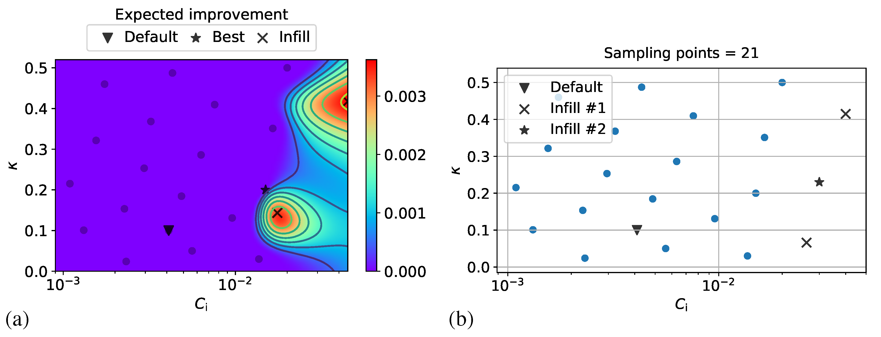
The “expected improvement” criterion is illustrated in Figure 6a. The two additional infill points using the “cl-mean” strategy are also indicated. On the one hand, the lower left infill point is near the previously found optimal solution, favoring hence the minimization of the true discrepancy function. On the other hand, the upper right infill point is focused on exploration of the design domain, in order to reduce the uncertainty of the surrogate. Based on the suggested locations, three more infill points (two during the first iteration, and another at the second iteration) are gradually included into the sampling plan (see Figure 6b).
The convergence of such adaptive optimization procedure is presented in Figure 7. The convergence criterion C given by Equation (6) decreases as more infill points are added into the sampling plan. We consider that convergence is achieved at the second iteration, where the maximal expected improvement can only further reduce the discrepancy by 0.4%.
3.3. Effect of the RSC Model Parameters Based on Uncoupled Simulations
Using the converged surrogate model, we now analyze the effect of the RSC model parameters when flow-fiber coupling is not considered. The final response surface is presented in Figure 8a. Using the information provided by the infill points, we observe that, when the inter-fiber interaction is overestimated, the difference between simulation and experimental data may increase. The -dependence of the discrepancy is also illustrated in Figure 8b for two fixed values. The uncertainty of the surrogate model is indicated by shaded regions using a 95% confidence level, i.e., . Due to the adequate placement of the sampling points, the surrogate model provides a sufficiently accurate approximation of the true discrepancy function, except possibly near the boundaries due to the lack of data. At these two different values of , the respective minimal values of discrepancy are also achieved at different , indicating some interaction between these two parameters.
Through optimization, we have thus reduced the discrepancy value from 0.223 when using the default parameter values to 0.174 when using the currently best or the optimal parameters (see Table 2). Note also the closeness between the “best” and the “optimal” solutions, which indicates a satisfying converged behavior. The optimal RSC parameters found here are close to those fitted with rheological experiments and used in [9,11,15].
To visually perceive the effect of optimization, the radial fiber orientation is presented in Figure 9. The default and the best RSC parameters are compared in the thickness direction at B and along the radial direction on the shell layer. On the one hand, the optimized parameters lead to a better agreement especially on the skin and in the shell layer. The core, on the other hand, is not much impacted. Concerning the radial evolution of fiber orientation, its behavior near the gate is not well predicted compared to the experimental data. It could be due to some modeling simplifications discussed in [22] and should be washed out as the flow advances. Nevertheless, the general decreasing trend is well captured and a quantitative agreement is achieved with the best found parameters.
As can be observed in Figure 8a, the optimal region that minimizes the discrepancy is approximately delimited by and , while the parameter, which governs the transient phase of fiber orientation evolution, plays a less important role within the range . In Figure 10, the discrepancy value is presented separately as a function of and , using the sampling points. The behavior of the parameter is obvious and more deterministic, indicating a stronger influence than the parameter which presents a quasi-random response especially for . A mathematical measure can be used to quantify the influence of each parameter on the objective function. It is discussed below, when we consider flow-fiber coupling effects.
3.4. Effect of Flow-Fiber Coupling During Optimization
Now, the effect of flow-fiber coupling with or without non-uniform fiber concentration effects [21,22] are considered during parametric optimization. For comparison concerns, the same final sampling points indicated in Figure 6b are used. The convergence criterion in Equation (6) confirms an acceptable converged behavior for the constructed surrogate response surface for all coupled simulations presented below.
In [22], it is found that a non-uniform fiber concentration enhances flow-fiber coupling and further decreases the discrepancy. The influence of the A parameter controlling the intensity of such coupling can only be perceived when the fiber volume fraction varies in space. With (compared to the default value ), the coupling effect is more important and also leads to a better agreement with experiment. In Figure 11a, the response surface in such strongly coupled situation is presented. According to the colorbars, the general discrepancy has decreased in the whole domain compared to the decoupled situation in Figure 8a. On the one hand, the region that maximizes discrepancy has moved downward and becomes more localized. On the other hand, the optimal region is slightly reduced in size and the optimal as well as the best solutions are also shifted upward. This indicates some non-trivial interaction between flow-fiber coupling and fiber orientation model parameters. Nevertheless, the optimal value of is still inside the previous interval.
At fixed , the discrepancy variation is presented in Figure 11b for the uncoupled case, the flow-fiber coupled case with nominal fiber concentration (coupled w/o ), the coupled case with non-uniform fiber concentration (coupled w/), and when is also included in the latter case. This presentation confirms what is found in [22] concerning flow-fiber coupling: a spatially-varying migration-induced fiber concentration contributes to an enhanced coupling behavior and leads to a better agreement with experiment. When fiber concentration is assumed at its nominal value, the coupling does reduce slightly the discrepancy, however the effect is less visible for the optimal parameters. Along with the corresponding discrepancies, they are summarized in Table 3. The relative reduction of discrepancy compared to the default value of 0.223 in Table 2 is also indicated. With maximum flow-fiber coupling (coupled w/, ), another 21% reduction can be obtained compared to the previous optimization without coupling effects.
Compared to the uncoupled optimization where fiber orientation prediction is mostly improved in the shell and skin layers (see again Figure 9), under flow-fiber coupling the gain from optimization is mostly concentrated in the core region (see Figure 12). On the one hand, the already optimized shell region is not much impacted by the coupling. On the other hand, the coupled optimization increases greatly the agreement in the core, due to a further slowed-down orientation kinetics. This result also agrees with our previous results reported in [21].
The benefit of flow-fiber coupling can also be perceived from the point of view of the global response surface. In Figure 13, the relative variation of the discrepancy compared to the uncoupled case is calculated at every sampling point (so using the same RSC parameters) and then combined to a response surface using the same kriging method. Apart from a localized area far away from the optimal region, flow-fiber coupling indeed leads to a further 20% reduction of discrepancy in a large portion of the domain. This illustrates again the importance of coupling in terms of fiber orientation prediction.
In Figure 14, we provide a novel representation of the flow-fiber coupling effect using parallel coordinates. Each sampling point (RSC parameters) is indicated by a dot and is connected by several segments of the same color. The effect of coupling is evaluated for each of the sampled RSC parameters, as we move from left to right in the horizontal direction. It can be seen that, as the coupling effect is enhanced gradually, the general discrepancy is also decreased.
Finally, to mathematically quantify the influence of the RSC parameters and the flow-fiber coupling effect, the “mutual information” measure implemented in the well-known machine learning toolkit scikit-learn [47] is used. This function characterizes the (linear and nonlinear) dependency between two random variables. While the two RSC parameters are continuous, the coupling effect is considered as a discrete one, with the four possible situations in Table 2 and Figure 14. The mutual information values are calculated in Table 4. As can be expected from Figure 10, the parameter explains a major (78%) variance of the discrepancy, while is indeed negligible. Flow-fiber coupling accounts for 22% of the total optimization effort and should not be neglected when one seeks to reduce the fiber orientation discrepancy between simulation and experiment.
Remark 1.
The influence of the reduction factor κ is unexpectedly evaluated to be 0%. Howeverm it indeed characterizes its quasi-random behavior illustrated in Figure 10b within the considered range . It can be expected that beyond this interval the effect of κ will be more obvious, even though it may increase the discrepancy.
4. Conclusions and Future Work
In this paper, a novel systematic approach to optimize the fiber orientation model parameters has been proposed. Constructed via Latin hypercube sampling and kriging, the surrogate response surface provides a global picture of how discrepancy varies in the parameter space. Its analytical nature permits a relatively straightforward identification of the optimal parameters. Adaptive infilling procedure can be employed to accelerate the minimization process and to decrease the uncertainty of the surrogate. The general procedure is not limited to the two-parameter RSC model and can be applied in the future to other advanced fiber orientation models with more parameters. Additional visualization techniques could be used to analyze such high-dimensional optimization. It is hoped that, when combined with a well-designed process and the associated flow kinematics representing injection molding [13], the systematic and robust optimization procedure described here may identify the correct parameters for fiber orientation kinetics during the molding process.
The discrepancy function to be minimized here measures the differences between the predicted and experimental fiber orientation data. Compared to previous approaches, here both the gapwise and the flow path directions are taken into account. The optimized solution hence possesses correct skin–shell–core structure and global orientation evolution throughout the part. It can be expected that the use of several measurement positions and height levels leads to a more robust optimization. For the same material, multiple injection molding experiments could also be conducted on different geometries. Using orientation measurements on several geometries in the same discrepancy function can also be considered in the future. Furthermore, in this paper, we are only interested in the fiber orientation predictions. We could have also performed a multiphysics optimization, where the differences in (non-uniform) fiber concentration between simulation and experiment are also included.
This paper also illustrates some non-trivial interaction between fiber orientation model parameters and flow-fiber coupling effects. The parametric fine-tuning of these orientation models mostly leads to a better agreement in the skin and shell regions, while the coupling effect via a fiber-dependent viscosity improves prediction in the core. The optimal region with minimal discrepancy in the parameter space may vary depending on whether flow-fiber coupling is taken into account. The influence of coupling on discrepancy reduction is also quantitively measured. Our results highlight the importance of coupling [21] and a non-uniform fiber concentration [22], along with the optimization of fiber orientation model parameters.
Author Contributions
T.L. conceived the methodology, performed the numerical simulations and drafted the manuscript; and J.-F.L. supervised the work and reviewed the manuscript.
Funding
This research was funded by the Région Île-de-France through the THERMOFIP research program (Pôle MOV’EO Convention 1709965).
Acknowledgments
The Moldflow API simulations presented in this paper could not be performed without the generous and unconditional help of Alain Benchissou from APLICIT.
Conflicts of Interest
The authors declare no conflict of interest. The funders had no role in the design of the study; in the collection, analyses, or interpretation of data; in the writing of the manuscript, or in the decision to publish the results.
Abbreviations
The following abbreviations are used in this manuscript:
| RSC | Reduction Strain Closure model |
| Coupled w/o | Flow-fiber coupled simulations with nominal fiber concentration |
| Coupled w/ | Flow-fiber coupled simulations with non-uniform fiber concentration |
References
- Papathanasiou, T.D. Flow-induced alignment in injection molding of fiber-reinforced polymer composites. In Flow-Induced Alignment in Composite Materials; Papthanasiou, T.D., Guell, D.C., Eds.; Woodhead Publishing: Cambridge, UK, 1997. [Google Scholar]
- Gupta, M.; Wang, K.K. Fiber orientation and mechanical properties of short-fiber-reinforced injection-molded composites: Simulated and experimental results. Polym. Compos. 1993, 14, 367–382. [Google Scholar] [CrossRef]
- Arif, M.F.; Saintier, N.; Meraghni, F.; Fitoussi, J.; Chemisky, Y.; Robert, G. Multiscale fatigue damage characterization in short glass fiber reinforced polyamide-66. Compos. Part B Eng. 2014, 61, 55–65. [Google Scholar] [CrossRef] [Green Version]
- Rolland, H.; Saintier, N.; Robert, G. Damage mechanisms in short glass fibre reinforced thermoplastic during in situ microtomography tensile tests. Compos. Part B Eng. 2016, 90, 365–377. [Google Scholar] [CrossRef]
- Folgar, F.; Tucker, C.L., III. Orientation behavior of fibers in concentrated suspensions. J. Reinf. Plast. Compos. 1984, 3, 98–119. [Google Scholar] [CrossRef]
- Advani, S.G.; Tucker, C.L., III. The use of tensors to describe and predict fiber orientation in short fiber composites. J. Rheol. 1987, 31, 751–784. [Google Scholar] [CrossRef]
- Phan-Thien, N.; Fan, X.J.; Tanner, R.I.; Zheng, R. Folgar-Tucker constant for a fibre suspension in a Newtonian fluid. J. Non-Newton. Fluid Mech. 2002, 103, 251–260. [Google Scholar] [CrossRef]
- Sepehr, M.; Ausias, G.; Carreau, P.J. Rheological properties of short fiber filled polypropylene in transient shear flow. J. Non-Newton. Fluid Mech. 2004, 123, 19–32. [Google Scholar] [CrossRef]
- Wang, J.; O’Gara, J.F.; Tucker , C.L., III. An objective model for slow orientation kinetics in concentrated fiber suspensions: Theory and rheological evidence. J. Rheol. 2008, 52, 1179–1200. [Google Scholar] [CrossRef]
- Eberle, A.P.R.; Baird, D.G.; Wapperom, P.; Vélez-García, G.M. Using transient shear rheology to determine material parameters in fiber suspension theory. J. Rheol. 2009, 53, 685–705. [Google Scholar] [CrossRef]
- Mazahir, S.M.; Vélez-García, G.M.; Wapperom, P.; Baird, D. Evolution of fibre orientation in radial direction in a center-gated disk: Experiments and simulation. Compos. Part A Appl. Sci. Manuf. 2013, 51, 108–117. [Google Scholar] [CrossRef]
- Perumal, V.; Gupta, R.K.; Bhattacharya, S.N.; Costa, F.S. Fiber orientation prediction in Nylon-6 glass fiber composites using transient rheology and 3-dimensional X-ray computed tomography. Polym. Compos. 2018. [Google Scholar] [CrossRef]
- Lambert, G.; Wapperom, P.; Baird, D. Obtaining short-fiber orientation model parameters using non-lubricated squeeze flow. Phys. Fluids 2017, 29, 121608. [Google Scholar] [CrossRef]
- Bay, R.S.; Tucker, C.L., III. Fiber orientation in simple injection moldings. Part II: Experimental results. Polym. Compos. 1992, 13, 332–341. [Google Scholar] [CrossRef]
- Vélez-García, G.M.; Mazahir, S.M.; Wapperom, P.; Baird, D.G. Simulation of Injection Molding Using a Model with Delayed Fiber Orientation. Int. Polym. Process. 2011, 26, 331–339. [Google Scholar] [CrossRef]
- Caton-Rose, P.; Hine, P.; Costa, F.; Jin, X.; Wang, J.; Parveen, B. Measurement and prediction of short glass fibre orientation in injection moulding composites. In Proceedings of the 15th European Conference on Composite Materials, Venice, Italy, 24–28 June 2012. [Google Scholar]
- Meyer, K.J.; Hofmann, J.T.; Baird, D.G. Prediction of short glass fiber orientation in the filling of an end-gated plaque. Compos. Part A Appl. Sci. Manuf. 2014, 62, 77–86. [Google Scholar] [CrossRef]
- van Haag, J.; Bontenackels, C.; Hopmann, C. Fiber orientation prediction of long fiber-reinforced thermoplastics: Optimization of model parameters. In Proceedings of the SPE ANTEC Conference, Orlando, FL, USA, 23–25 March 2015. [Google Scholar]
- Tseng, H.C.; Chang, R.Y.; Hsu, C.H. Improved fiber orientation predictions for injection molded fiber composites. Compos. Part A Appl. Sci. Manuf. 2017, 99, 65–75. [Google Scholar] [CrossRef]
- Kleindel, S.; Salaberger, D.; Eder, R.; Schretter, H.; Hochenauer, C. Prediction and Validation of Short Fiber Orientation in a Complex Injection Molded Part with Chunky Geometry. Int. Polym. Process. 2015, 30, 366–380. [Google Scholar] [CrossRef]
- Li, T.; Luyé, J.F. Flow-fiber coupled viscosity in injection molding simulations of short fiber reinforced thermoplastics. Int. Polym. Process. 2018. Available online: https://hal.archives-ouvertes.fr/hal-01683052 (accessed on 18 December 2018).
- Li, T.; Luyé, J.F. Flow-fiber coupled injection molding simulations with non-uniform fiber concentration effects. 2018, in press. [Google Scholar]
- Wang, J.; Cook, P.; Bakharev, A.; Costa, F.; Astbury, D. Prediction of fiber orientation in injection-molded parts using three-dimensional simulations. AIP Conf. Proc. 2016, 1713, 40007. [Google Scholar] [CrossRef] [Green Version]
- Forrester, A.; Keane, A.; Keane, A. Engineering Design via Surrogate Modelling: A Practical Guide; John Wiley Sons: Hoboken, NJ, USA, 2008. [Google Scholar]
- Simpson, T.W.; Poplinski, J.D.; Koch, P.N.; Allen, J.K. Metamodels for computer-based engineering design: Survey and recommendations. Eng. Comput. 2001, 17, 129–150. [Google Scholar] [CrossRef]
- Autodesk. Autodesk Moldflow 2019 Technology Preview: What Is New; Autodesk Australia Pty Ltd.: Kilsyth, VIC, Australia, 2018. [Google Scholar]
- Tucker, C.L., III. Flow regimes for fiber suspensions in narrow gaps. J. Non-Newton. Fluid Mech. 1991, 39, 239–268. [Google Scholar] [CrossRef]
- Costa, F.; Cook, P.; Pickett, D. A Framework for Viscosity Model Research in Injection Molding Simulation, Including Pressure and Fiber Orientation Dependence. In Proceedings of the SPE ANTEC Conference, Orlando, FL, USA, 23–25 March 2015. [Google Scholar]
- Goris, S.; Osswald, T.A. Process-induced fiber matrix separation in long fiber-reinforced thermoplastics. Compos. Part A Appl. Sci. Manuf. 2018, 105, 321–333. [Google Scholar] [CrossRef]
- Morris, J.F. A review of microstructure in concentrated suspensions and its implications for rheology and bulk flow. Rheol. Acta 2009, 48, 909–923. [Google Scholar] [CrossRef]
- Costa, F. Autodesk Moldflow Insight: Solver Enhancements and Research Directions. In Proceedings of the Benelux Autodesk Moldflow User Meeting, Eindhoven, The Netherlands, 24 June 2016. [Google Scholar]
- Tseng, H.C.; Chang, R.Y.; Hsu, C.H. Predictions of fiber concentration in injection molding simulation of fiber-reinforced composites. J. Thermoplast. Compos. Mater. 2017. [Google Scholar] [CrossRef]
- VerWeyst, B.E.; Tucker, C.L., III; Foss, P.H.; O’Gara, J.F. Fiber Orientation In 3-d Injection Molded Features: Prediction and Experiment. Int. Polym. Process. 1999, 14, 409–420. [Google Scholar] [CrossRef]
- Vélez-García, G.M.; Wapperom, P.; Baird, D.G.; Aning, A.O.; Kunc, V. Unambiguous orientation in short fiber composites over small sampling area in a center-gated disk. Compos. Part A Appl. Sci. Manuf. 2012, 43, 104–113. [Google Scholar] [CrossRef]
- Autodesk. Autodesk Moldflow Insight 2017 R2: Fiber orientation Accuracy Validation Report; Autodesk Australia Pty Ltd.: Kilsyth, VIC, Australia, 2016. [Google Scholar]
- Jones, D.R. A Taxonomy of Global Optimization Methods Based on Response Surfaces. J. Glob. Optim. 2001, 21, 345–383. [Google Scholar] [CrossRef]
- McKay, M.D.; Beckman, R.J.; Conover, W.J. A Comparison of Three Methods for Selecting Values of Input Variables in the Analysis of Output from a Computer Code. Technometrics 1979, 21, 239–245. [Google Scholar] [CrossRef]
- Sacks, J.; Welch, W.J.; Mitchell, T.J.; Wynn, H.P. Design and Analysis of Computer Experiments. Stat. Sci. 1989, 4, 409–423. [Google Scholar] [CrossRef]
- Morris, M.D.; Mitchell, T.J. Exploratory designs for computational experiments. J. Stat. Plan. Inference 1995, 43, 381–402. [Google Scholar] [CrossRef]
- Jin, R.; Chen, W.; Sudjianto, A. An efficient algorithm for constructing optimal design of computer experiments. J. Stat. Plan. Inference 2005, 134, 268–287. [Google Scholar] [CrossRef]
- Vu, K.K.; d’Ambrosio, C.; Hamadi, Y.; Liberti, L. Surrogate-based methods for black-box optimization. Int. Trans. Oper. Res. 2016, 24, 393–424. [Google Scholar] [CrossRef]
- Jones, D.R.; Schonlau, M.; Welch, W.J. Efficient Global Optimization of Expensive Black-Box Functions. J. Glob. Optim. 1998, 13, 455–492. [Google Scholar] [CrossRef]
- Gao, Y.; Wang, X. Surrogate-based process optimization for reducing warpage in injection molding. J. Mater. Process. Technol. 2009, 209, 1302–1309. [Google Scholar] [CrossRef]
- Ginsbourger, D.; Riche, R.L.; Carraro, L. Kriging Is Well-Suited to Parallelize Optimization. In Computational Intelligence in Expensive Optimization Problems; Springer: Berlin/Heidelberg, Germany, 2010; pp. 131–162. [Google Scholar]
- Wales, D.J.; Doye, J.P.K. Global Optimization by Basin-Hopping and the Lowest Energy Structures of Lennard-Jones Clusters Containing up to 110 Atoms. J. Phys. Chem. A 1997, 101, 5111–5116. [Google Scholar] [CrossRef] [Green Version]
- Jones, E.; Oliphant, T.; Peterson, P. SciPy: Open Source Scientific Tools for Python. 2001. Available online: http://www.scipy.org/ (accessed on 18 December 2018).
- Pedregosa, F.; Varoquaux, G.; Gramfort, A.; Michel, V.; Thirion, B.; Grisel, O.; Blondel, M.; Prettenhofer, P.; Weiss, R.; Dubourg, V.; et al. Scikit-learn: Machine Learning in Python. J. Mach. Learn. Res. 2011, 12, 2825–2830. [Google Scholar]
Figure 1.
Optimization flowchart to minimize the discrepancy between numerical and the experimental fiber orientation results via surrogate modeling.
Figure 1.
Optimization flowchart to minimize the discrepancy between numerical and the experimental fiber orientation results via surrogate modeling.

Figure 2.
Illustration of different discrepancy measures between the predicted and the measured gapwise fiber orientation: one based on the the difference throughout the thickness direction (shaded region), and the other based on the thickness-averaged values (dotted lines).
Figure 2.
Illustration of different discrepancy measures between the predicted and the measured gapwise fiber orientation: one based on the the difference throughout the thickness direction (shaded region), and the other based on the thickness-averaged values (dotted lines).

Figure 3.
Geometrical parameters and measurement positions of the center gated plate: (a) 3D view with B and C two measurement radial positions along the thickness direction; and (b) cut view with three additional measurement height levels (shell, transition and core layers) along the radial direction.

Figure 4.
Initial sampling plan for in the design space. The default parameter value of Moldflow as well as the values used in [9,11] are also indicated.

Figure 5.
(a) Discrepancy response surface; and (b) standard deviation (uncertainty) based on the initial sampling plan.
Figure 5.
(a) Discrepancy response surface; and (b) standard deviation (uncertainty) based on the initial sampling plan.

Figure 6.
(a) Expected improvement predicted by the surrogate model; and (b) infill points added to the initial sampling plan.
Figure 6.
(a) Expected improvement predicted by the surrogate model; and (b) infill points added to the initial sampling plan.

Figure 7.
Convergence of the surrogate model.

Figure 8.
(a) Converged discrepancy response with uncoupled simulations; and (b) discrepancy variation along the lines and , with a confidence level of 95% represented by shaded regions.
Figure 8.
(a) Converged discrepancy response with uncoupled simulations; and (b) discrepancy variation along the lines and , with a confidence level of 95% represented by shaded regions.

Figure 9.
Radial fiber orientation (a) at B and (b) in the shell region, using the default or the best RSC parameters, without flow-fiber coupling.
Figure 9.
Radial fiber orientation (a) at B and (b) in the shell region, using the default or the best RSC parameters, without flow-fiber coupling.

Figure 10.
Discrepancy as a function of (a) and (b) without flow-fiber coupling.

Figure 11.
(a) Response surface with flow-fiber coupling, non-uniform fiber concentration effects (coupled w/) and ; and (b) discrepancy as a function of at , for several coupling situations.
Figure 11.
(a) Response surface with flow-fiber coupling, non-uniform fiber concentration effects (coupled w/) and ; and (b) discrepancy as a function of at , for several coupling situations.

Figure 12.
Radial fiber orientation (a) in the shell and (b) in the core region, using the default or the best RSC parameters, with or without flow-fiber coupling.
Figure 12.
Radial fiber orientation (a) in the shell and (b) in the core region, using the default or the best RSC parameters, with or without flow-fiber coupling.

Figure 13.
Relative discrepancy variation (a larger negative value stands for a greater reduction of discrepancy) using flow-fiber coupling, non-uniform concentration effects and , compared to the uncoupled case.
Figure 13.
Relative discrepancy variation (a larger negative value stands for a greater reduction of discrepancy) using flow-fiber coupling, non-uniform concentration effects and , compared to the uncoupled case.

Figure 14.
Effect of flow-fiber coupling using parallel coordinates, where each line with the same color connects the same RSC parameters (same sampling point) and evolves according to flow-fiber coupling situation.
Figure 14.
Effect of flow-fiber coupling using parallel coordinates, where each line with the same color connects the same RSC parameters (same sampling point) and evolves according to flow-fiber coupling situation.


Table 1.
Comparison between different discrepancy measures for the case considered in Figure 2.
Table 1.
Comparison between different discrepancy measures for the case considered in Figure 2.
| Using (2) | Using (3) | |
|---|---|---|
| Discrepancy | 12% | 2.9% |
Table 2.
Discrepancy values using the default or optimized RSC parameters without fiber-flow coupling.
Table 2.
Discrepancy values using the default or optimized RSC parameters without fiber-flow coupling.
| RSC Parameters | Discrepancy | |
|---|---|---|
| Default | 0.223 | |
| Best | 0.174 | |
| Optimal | 0.174 |
Table 3.
Optimal parameters for the RSC fiber orientation model with or without fiber-flow coupling.
Table 3.
Optimal parameters for the RSC fiber orientation model with or without fiber-flow coupling.
| Optimal Parameters | Discrepancy | Compared to “Default” | |
|---|---|---|---|
| Uncoupled | 0.174 | −22% | |
| Coupled w/o | 0.170 | −24% | |
| Coupled w/ | 0.149 | −33% | |
| Coupled w/, | 0.127 | −43% |
Table 4.
Relative influence on the discrepancy measured by the mutual information.
| Interaction Coefficient | Reduction Factor | Flow-Fiber Coupling |
|---|---|---|
| 78% | 0% | 22% |
© 2018 by the authors. Licensee MDPI, Basel, Switzerland. This article is an open access article distributed under the terms and conditions of the Creative Commons Attribution (CC BY) license (http://creativecommons.org/licenses/by/4.0/).
Share and Cite
MDPI and ACS Style
Li, T.; Luyé, J.-F. Optimization of Fiber Orientation Model Parameters in the Presence of Flow-Fiber Coupling. J. Compos. Sci. 2018, 2, 73. https://doi.org/10.3390/jcs2040073
AMA Style
Li T, Luyé J-F. Optimization of Fiber Orientation Model Parameters in the Presence of Flow-Fiber Coupling. Journal of Composites Science. 2018; 2(4):73. https://doi.org/10.3390/jcs2040073
Chicago/Turabian StyleLi, Tianyi, and Jean-François Luyé. 2018. "Optimization of Fiber Orientation Model Parameters in the Presence of Flow-Fiber Coupling" Journal of Composites Science 2, no. 4: 73. https://doi.org/10.3390/jcs2040073