
A Data Driven Modelling Approach for the Strain Rate Dependent 3D Shear Deformation and Failure of Thermoplastic Fibre Reinforced Composites: Experimental Characterisation and Deriving Modelling Parameters


Abstract
:1. Introduction
2. Experimental Methodology
2.1. Material Configuration and Specimen Preparation
2.2. Experimental Setup and Testing Program
3. Experimental Results
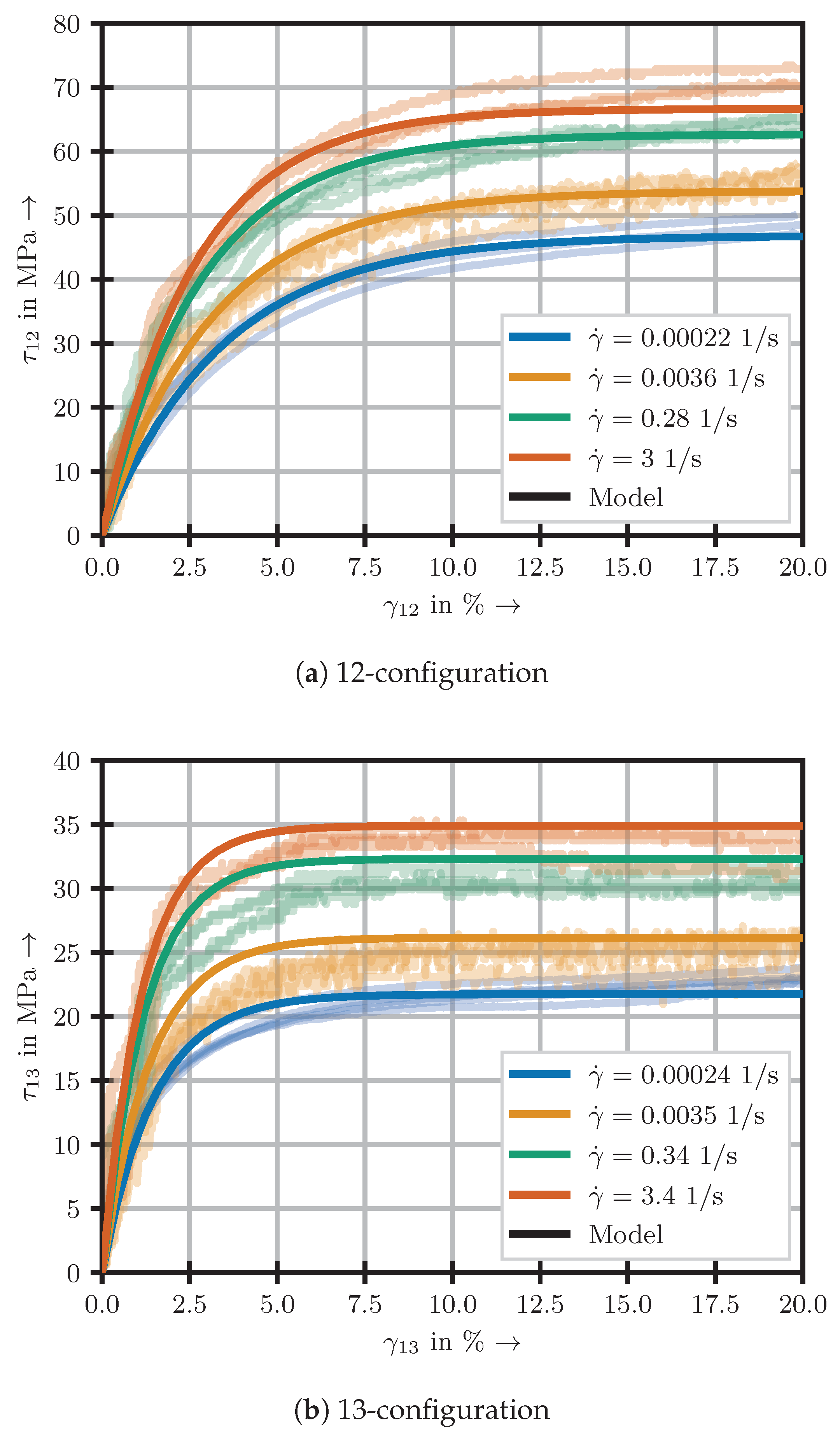
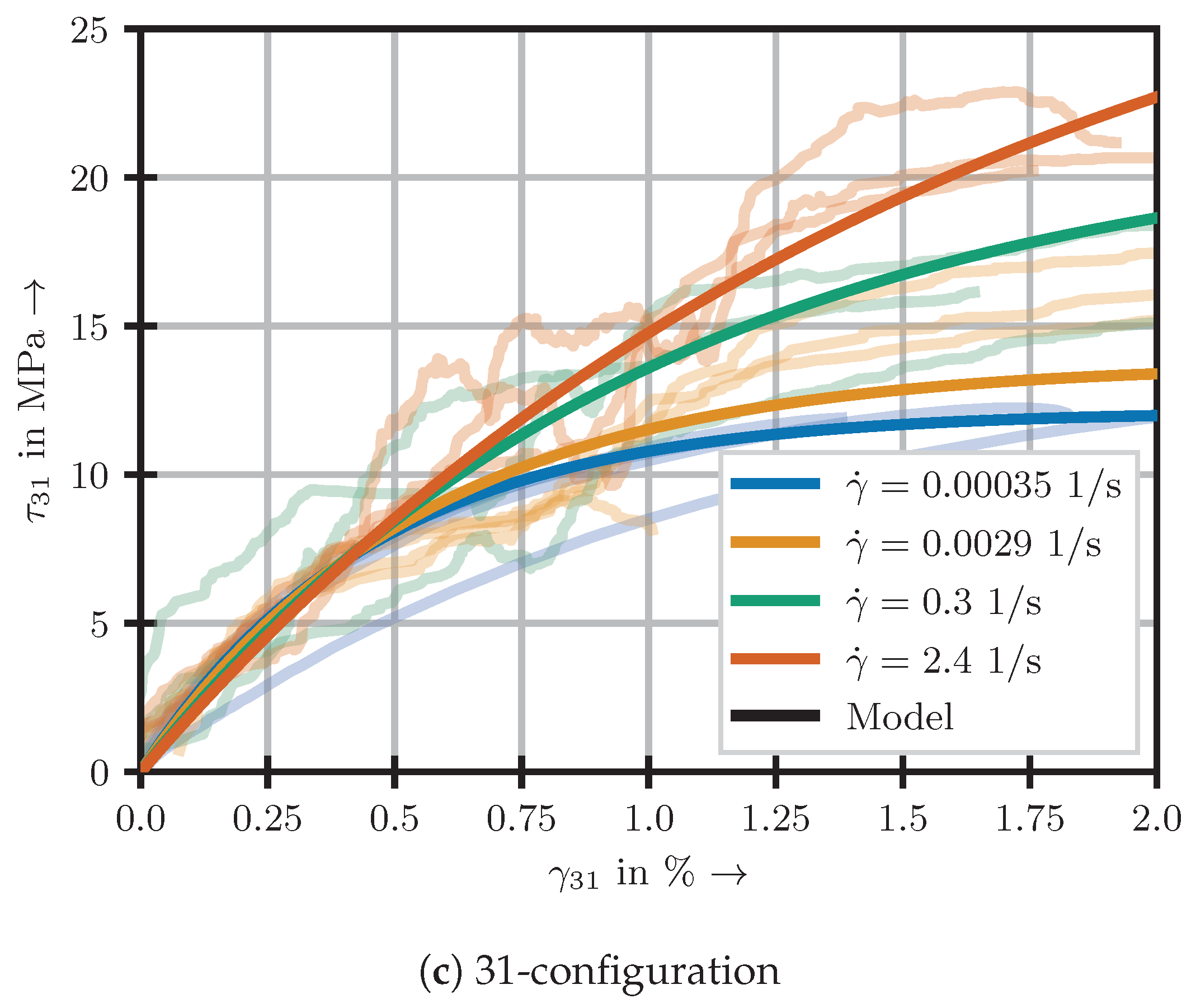
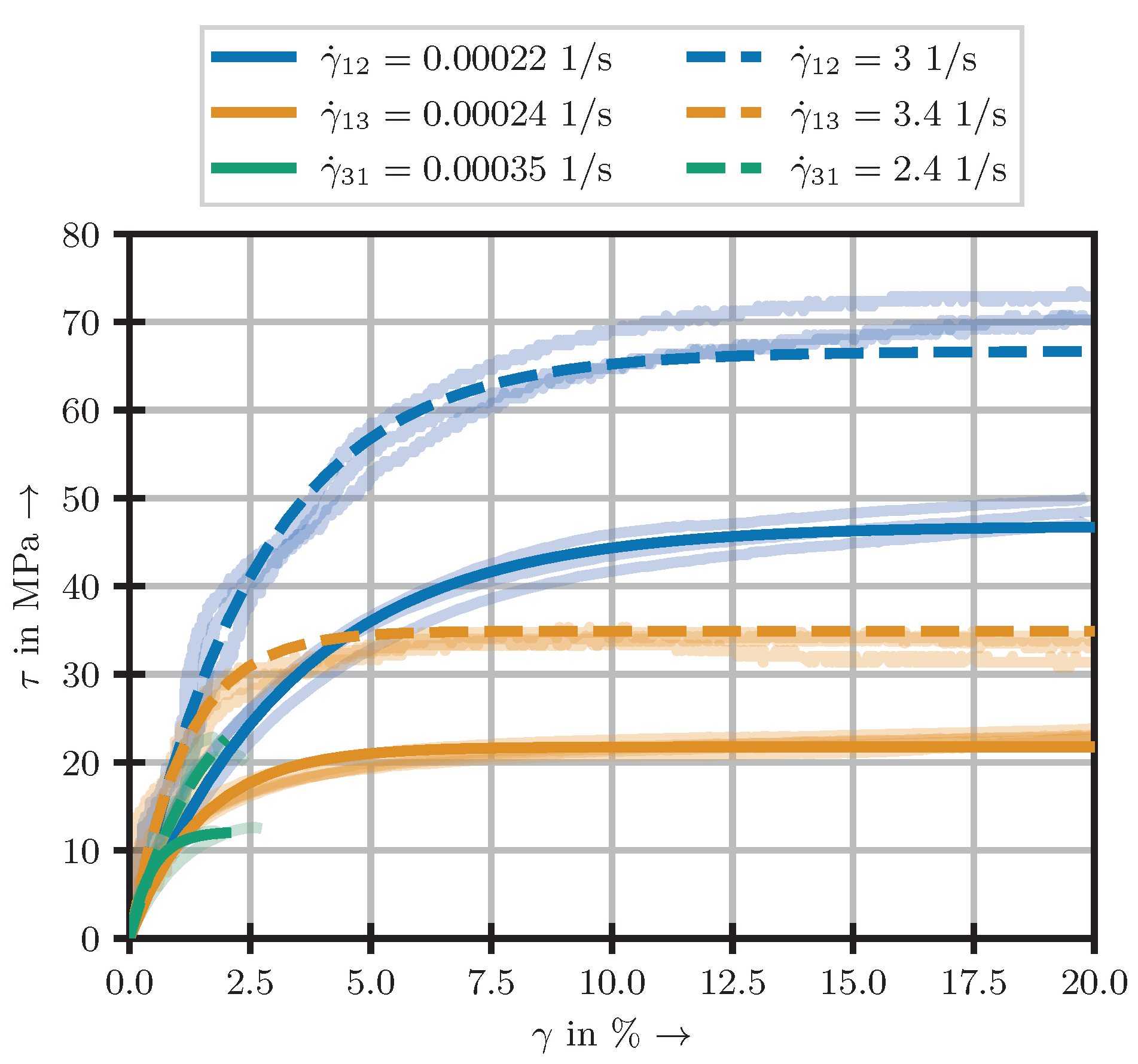
3.1. Stress–Strain Behaviour and Experimental Classification
3.2. Failure and Fracture Behaviour
4. Material Modelling and Property Identification
- data driven (DD): A closed formulation describing the entire experimental curves by coherent formulae with the determining parameters being the material’s characteristics.
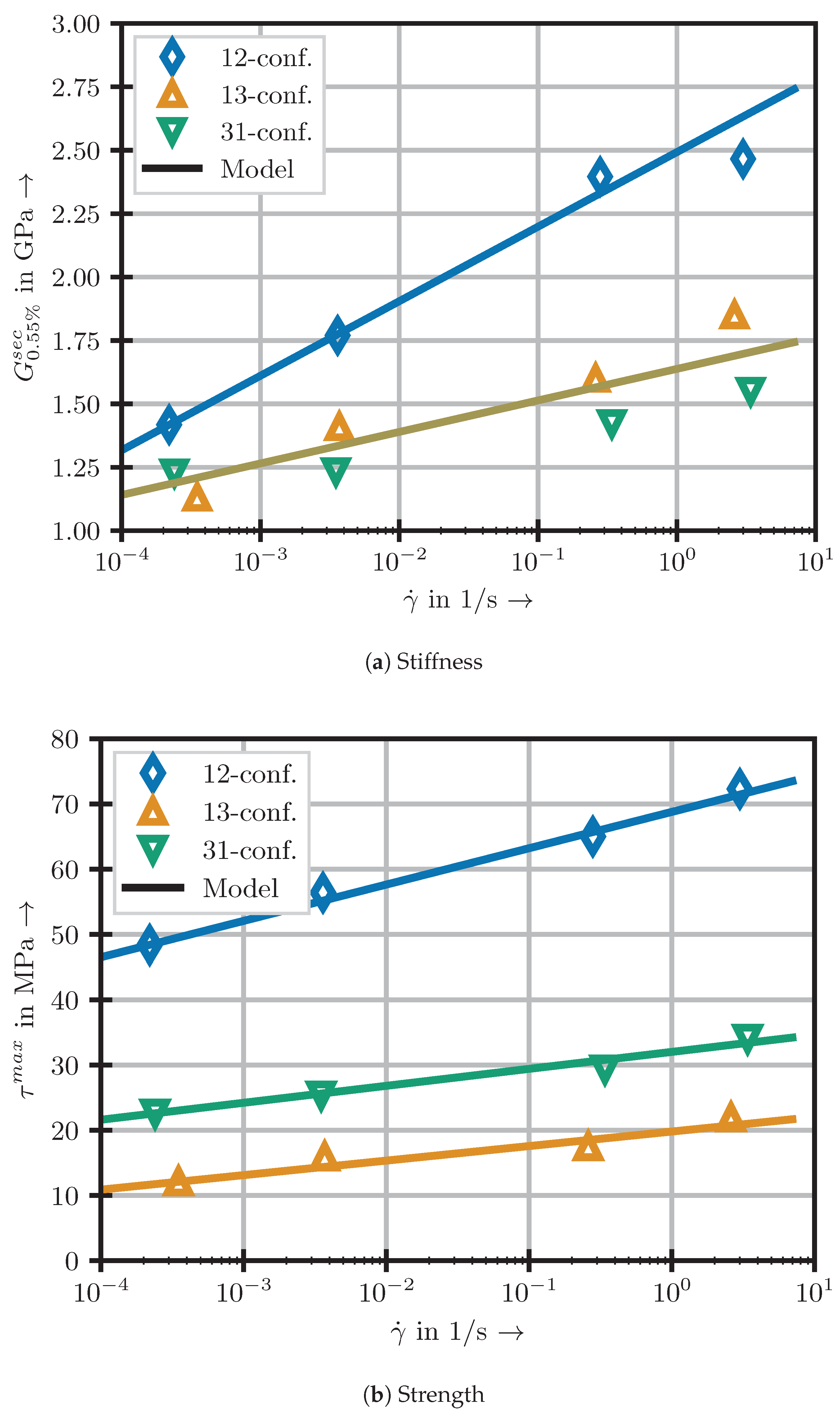
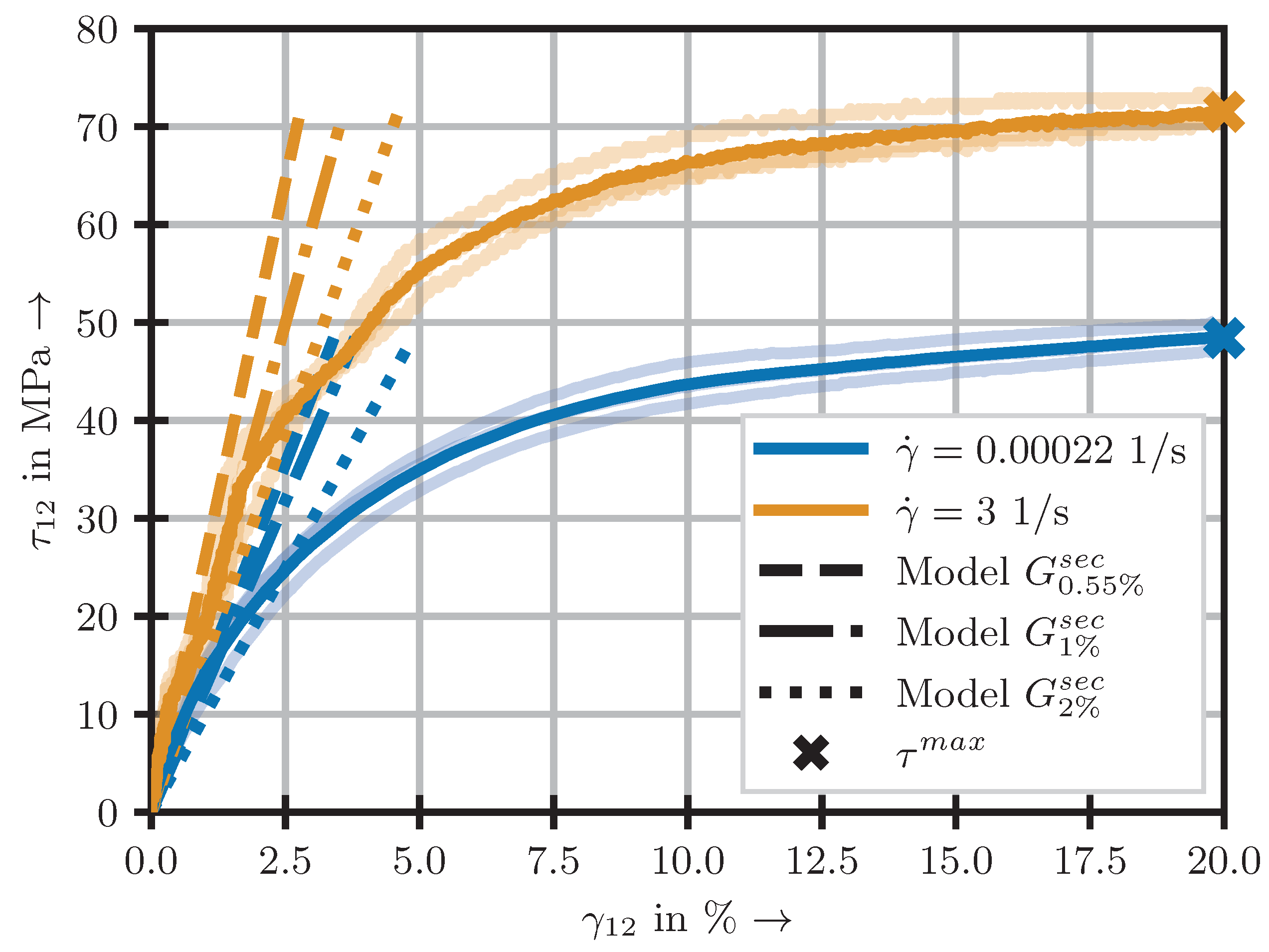
4.1. Modulus and Strength Based (MaS) Approach
4.1.1. Determination of Engineering Constants
4.1.2. Strain Rate Dependency and Model Parameters
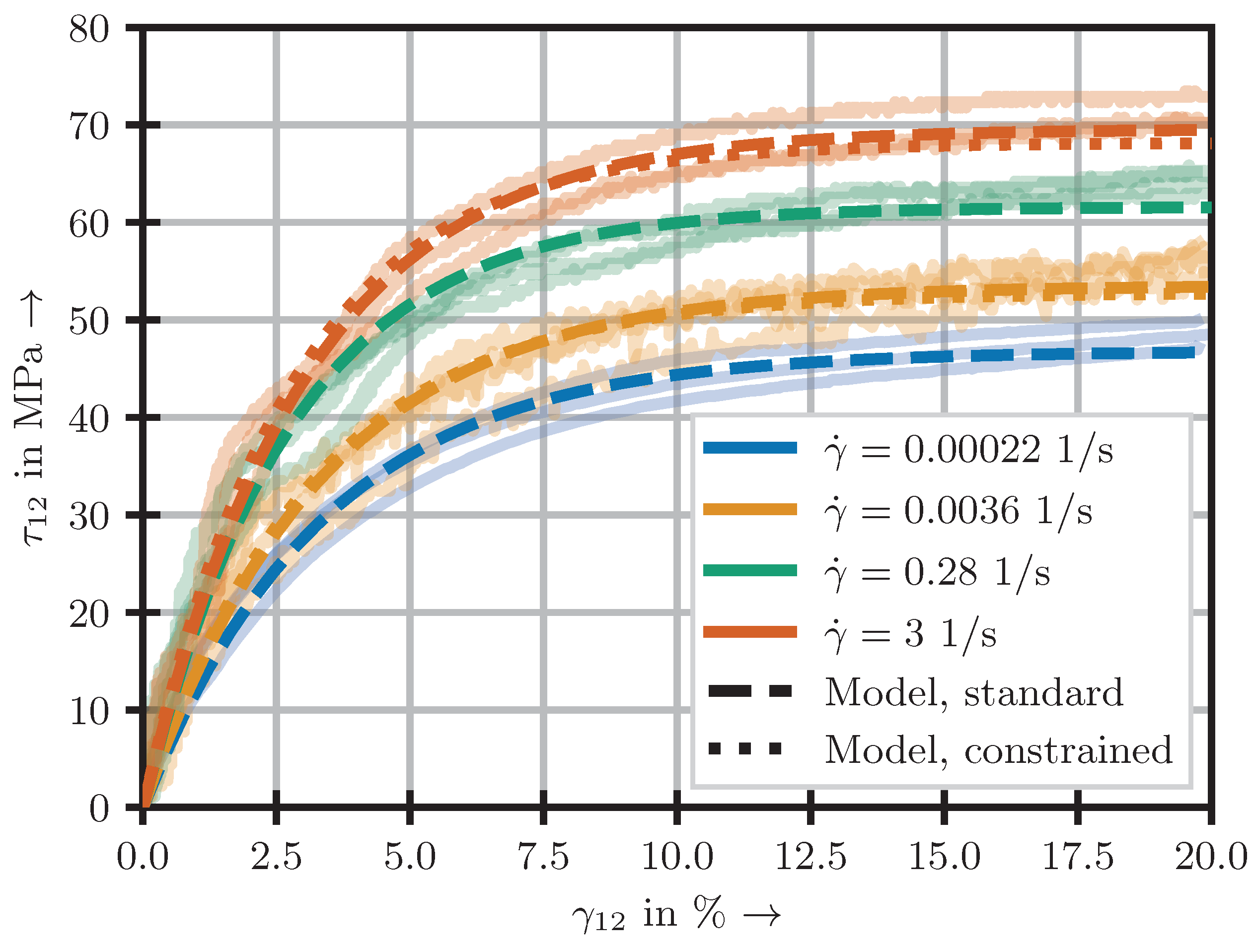
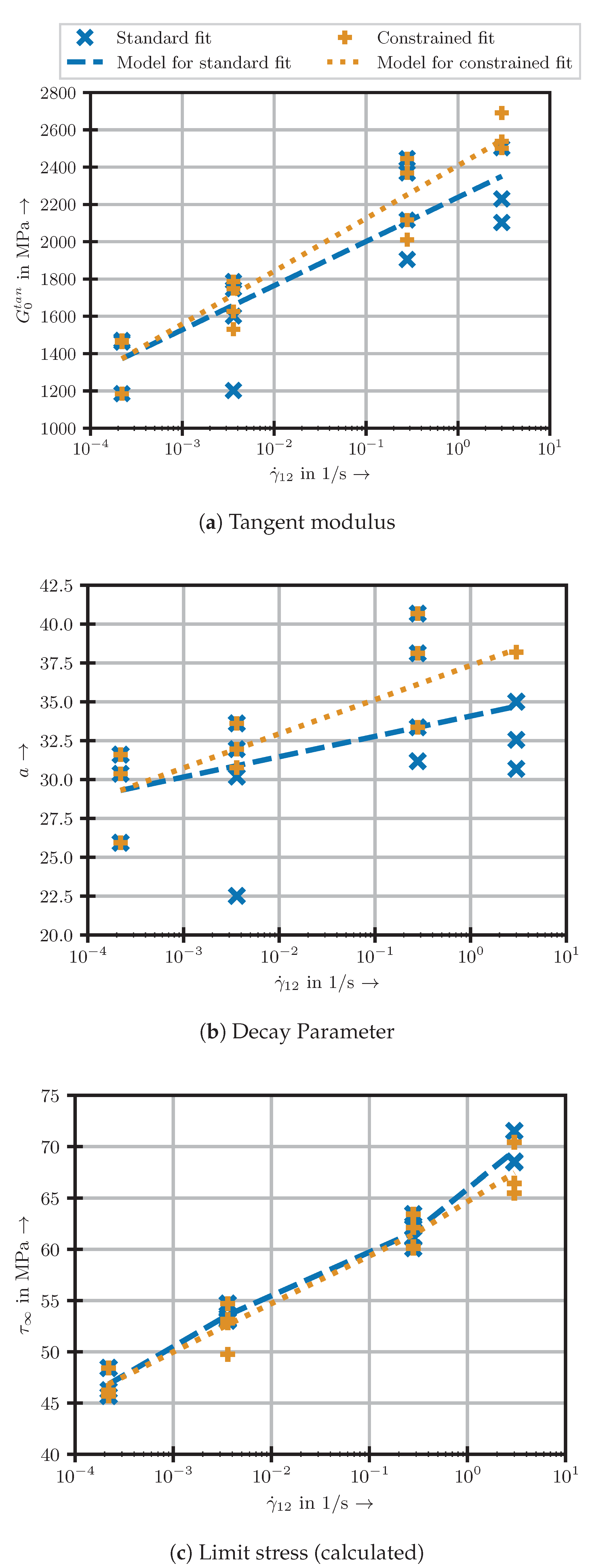
4.2. Data Driven (DD) Approach
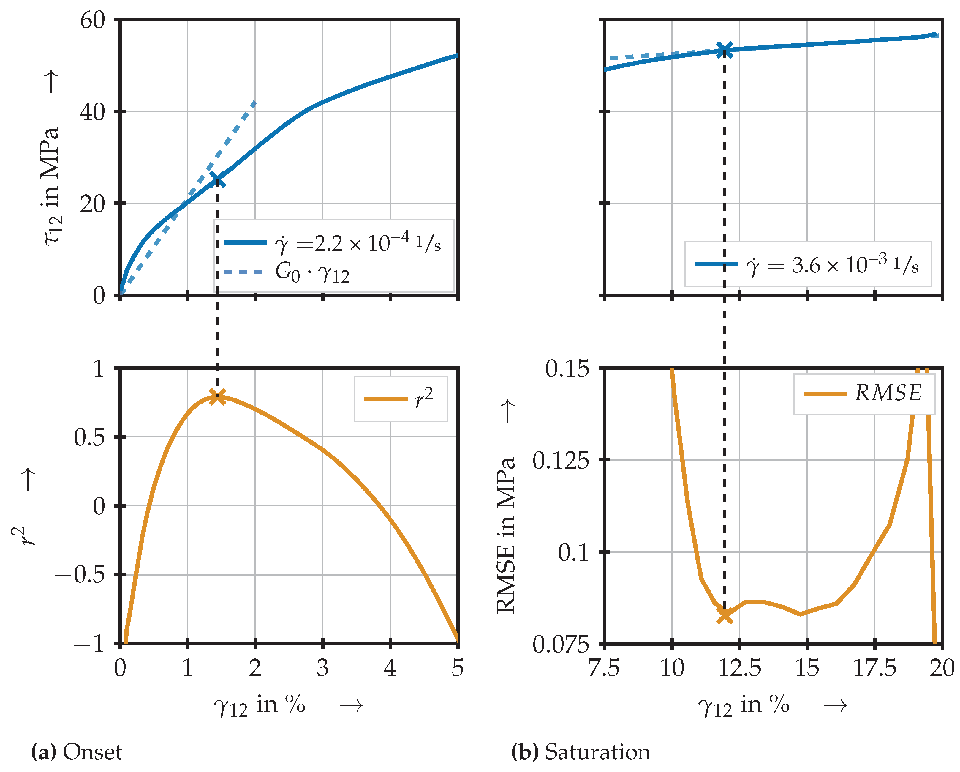
4.2.1. Determination of Material Characteristics
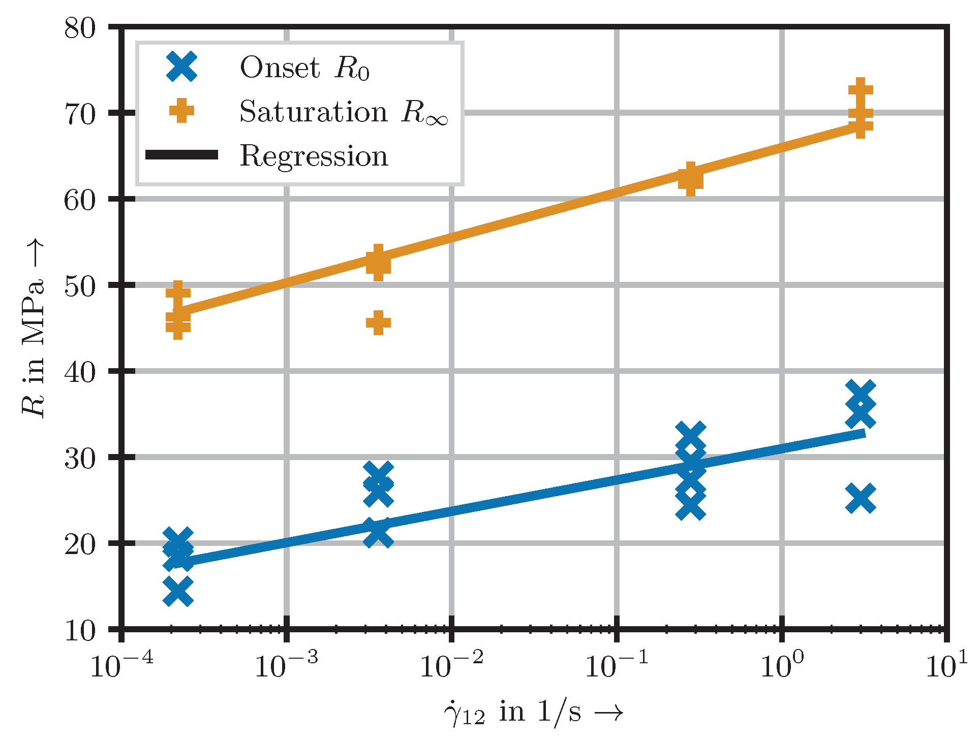
4.2.2. Modelling of the Strain Rate Dependency
4.3. Determining the Range of Validity of the Material Modelling Approaches
5. Discussion
5.1. Strain Rate and Configuration Dependent Experimental Characterisation
5.2. Presented Modelling Approaches
5.2.1. Modulus and Strength Based (MaS) Approach
5.2.2. Data Driven (DD) Approach
5.3. Interpretability of the Nonlinearities
6. Conclusions and Outlook
Author Contributions
Funding
Institutional Review Board Statement
Informed Consent Statement
Data Availability Statement
Acknowledgments
Conflicts of Interest
Abbreviations
| DD | data driven |
| DIC | digital image correlation |
| FEA | finite element analysis |
| FRP | fibre reinforced plastic |
| GF/PP | E-glass fibre polypropylene |
| MaS | modulus and strength based |
| MKF | multi-layered weft knitted fabric |
| PP | polypropylene |
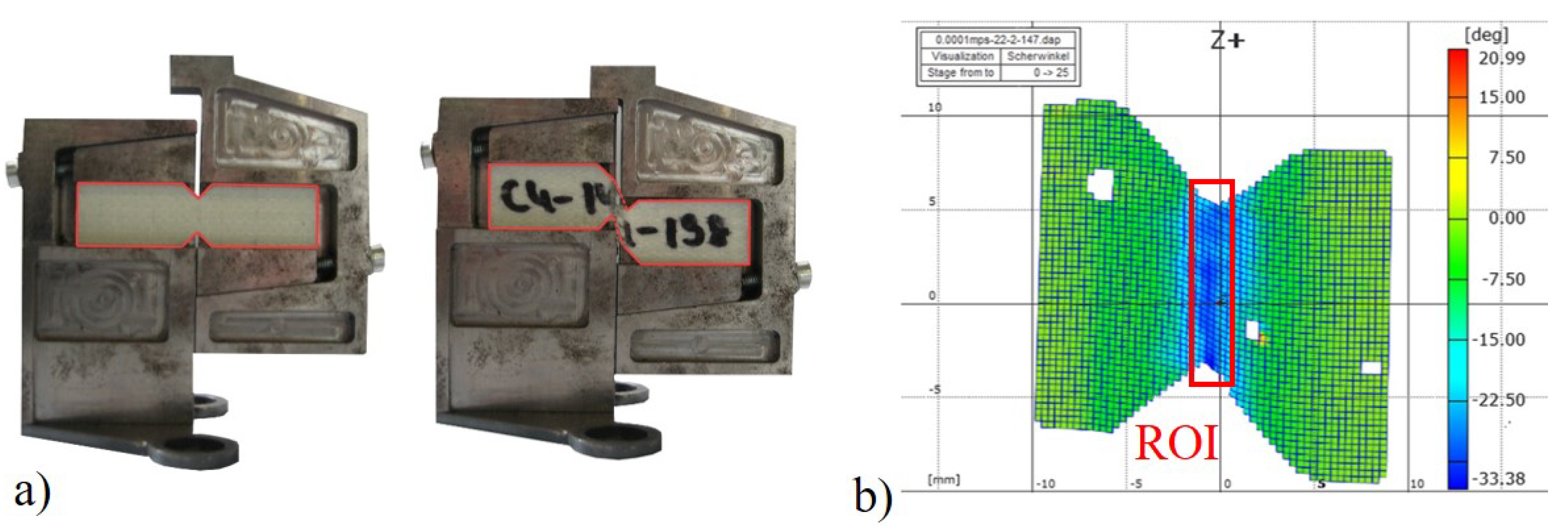
| ROI | region of interest |
| SHPB | split Hopkinson pressure bar |
| TT | through thickness |
References
- Sarfraz, M.S.; Hong, H.; Kim, S.S. Recent developments in the manufacturing technologies of composite components and their cost-effectiveness in the automotive industry: A review study. Compos. Struct. 2021, 266, 113864. [Google Scholar] [CrossRef]
- Böhm, R.; Hornig, A.; Weber, T.; Grüber, B.; Gude, M. Experimental and Numerical Impact Analysis of Automotive Bumper Brackets Made of 2D Triaxially Braided CFRP Composites. Materials 2020, 13, 3554. [Google Scholar] [CrossRef] [PubMed]
- Zimmermann, N.; Wang, P.H. A review of failure modes and fracture analysis of aircraft composite materials. Eng. Fail. Anal. 2020, 115, 104692. [Google Scholar] [CrossRef]
- Haufe, A.; Cavariani, S.; Liebold, C.; Usta, T.; Kotzakolios, T.; Giannaros, E.; Kostopoulos, V.; Hornig, A.; Gude, M.; Djordjevic, N.; et al. On Composite Model Calibration for Extreme Impact Loading Exemplified on Aerospace Structures. In Proceedings of the 16th LS-Dyna International Users Conference, Aerospace, LSTC-Ansys, Virtual Event, 10–11 June 2020. [Google Scholar]
- Olsson, R. A survey of test methods for multiaxial and out-of-plane strength of composite laminates. Compos. Sci. Technol. 2011, 71, 773–783. [Google Scholar] [CrossRef] [Green Version]
- Gude, M.; Schirner, R.; Weck, D.; Dohmen, E.; Andrich, M. Through-thickness compression testing of fabric reinforced composite materials: Adapted design of novel compression stamps. Polym. Test. 2016, 56, 269–276. [Google Scholar] [CrossRef]
- Kanno, T.; Kurita, H.; Suzuki, M.; Tamura, H.; Narita, F. Numerical and Experimental Investigation of the Through-Thickness Strength Properties of Woven Glass Fiber Reinforced Polymer Composite Laminates under Combined Tensile and Shear Loading. J. Compos. Sci. 2020, 4, 112. [Google Scholar] [CrossRef]
- Jalali, S.J.; Taheri, F. A New Test Method for Measuring the Longitudinal and Shear Moduli of Fiber Reinforced Composites. J. Compos. Mater. 1999, 33, 2134–2160. [Google Scholar] [CrossRef] [Green Version]
- Yoneyama, S.; Ifju, P.G.; Rohde, S.E. Identifying through-thickness material properties of carbon-fiber-reinforced plastics using the virtual fields method combined with moiré interferometry. Adv. Compos. Mater. 2018, 27, 1–17. [Google Scholar] [CrossRef]
- Gude, M.; Hufenbach, W.; Andrich, M.; Mertel, A.; Schirner, R. Modified V-notched rail shear test fixture for shear characterisation of textile-reinforced composite materials. Polym. Test. 2015, 43, 147–153. [Google Scholar] [CrossRef]
- Stojcevski, F.; Hilditch, T.; Henderson, L.C. A modern account of Iosipescu testing. Compos. Part Appl. Sci. Manuf. 2018, 107, 545–554. [Google Scholar] [CrossRef]
- Guseinov, K.; Kudryavtsev, O.; Bezmelnitsyn, A.; Sapozhnikov, S. Determination of Interlaminar Shear Properties of Fibre-Reinforced Composites under Biaxial Loading: A New Experimental Approach. Polymers 2022, 14, 2575. [Google Scholar] [CrossRef] [PubMed]
- Hsiao, H.M.; Daniel, I.M.; Cordes, R.D. Strain Rate Effects on the Transverse Compressive and Shear Behavior of Unidirectional Composites. J. Compos. Mater. 1999, 33, 1620–1642. [Google Scholar] [CrossRef]
- Zhao, Z.; Liu, P.; Dang, H.; Nie, H.; Guo, Z.; Zhang, C.; Li, Y. Effects of loading rate and loading direction on the compressive failure behavior of a 2D triaxially braided composite. Int. J. Impact Eng. 2021, 156, 103928. [Google Scholar] [CrossRef]
- Hufenbach, W.; Langkamp, A.; Hornig, A.; Zscheyge, M.; Bochynek, R. Analysing and modelling the 3D shear damage behaviour of hybrid yarn textile-reinforced thermoplastic composites. Compos. Struct. 2011, 94, 121–131. [Google Scholar] [CrossRef]
- Hufenbach, W.; Langkamp, A.; Gude, M.; Ebert, C.; Hornig, A.; Nitschke, S.; Böhm, H. Characterisation of Strain rate Dependent Material Properties of Textile Reinforced Thermoplastics for Crash and Impact Analysis. Procedia Mater. Sci. 2013, 2, 204–211. [Google Scholar] [CrossRef] [Green Version]
- Hassan, J.; O’Higgins, R.M.; McCarthy, C.T.; Toso, N.; McCarthy, M.A. Mesoscale modelling of extended bearing failure in tension-absorber joints. Int. J. Mech. Sci. 2020, 182, 105777. [Google Scholar] [CrossRef]
- Johnson, G.R.; Cook, W.H. Fracture characteristics of three metals subjected to various strains, strain rates, temperatures and pressures. Eng. Fract. Mech. 1985, 21, 31–48. [Google Scholar] [CrossRef]
- Zscheyge, M.; Böhm, R.; Hornig, A.; Gerritzen, J.; Gude, M. Rate dependent nonlinear mechanical behaviour of continuous fibre-reinforced thermoplastic composites – Experimental characterisation and viscoelastic-plastic damage modelling. Mater. Des. 2020, 193, 108827. [Google Scholar] [CrossRef]
- Böhm, R.; Gude, M.; Hufenbach, W. A phenomenologically based damage model for textile composites with crimped reinforcement. Compos. Sci. Technol. 2010, 70, 81–87. [Google Scholar] [CrossRef]
- Gude, M.; Hufenbach, W.; Ebert, C. The strain-rate-dependent material and failure behaviour of 2D and 3D non-crimp glass-fibre-reinforced composites. Mech. Compos. Mater. 2009, 45, 467–476. [Google Scholar] [CrossRef]
- Diestel, O.; Godau, U.; Offermann, P. Biaxially reinforced multilayer weft knitted fabrics - a new textile structure for composite reinforcement. In Proceedings of the 30th International SAMPE Technical Conference, San Antonio, TX, USA, 21–24 October 1998; pp. 40–47. [Google Scholar]
- Hufenbach, W.; Gude, M.; Ebert, C.; Zscheyge, M.; Hornig, A. Strain rate dependent low velocity impact response of layerwise 3D-reinforced composite structures. Int. J. Impact Eng. 2011, 38, 358–368. [Google Scholar] [CrossRef]
- ASTM D5379/D5379M-19e1; Standard Test Method for Shear Properties of Composite Materials by the V-Notched Beam Method. ASTM International: West Conshohocken, PA, USA, 2019. [CrossRef]
- DIN EN ISO 14129:1998-02; Fibre-Reinforced Plastic Composites—Determination of the In-Plane Shear Stress/Shear Strain Response, Including the In-Plane Shear Modulus and Strength, by ±45° Tension Test Method (ISO 14129:1997). Beuth Verlag: Berlin, Germany, 1998. [CrossRef]
- Pantalé, O.; Bacaria, J.L.; Dalverny, O.; Rakotomalala, R.; Caperaa, S. 2D and 3D numerical models of metal cutting with damage effects. Comput. Methods Appl. Mech. Eng. 2004, 193, 4383–4399. [Google Scholar] [CrossRef] [Green Version]
- Krasauskas, P.; Kilikevičius, S.; Česnavičius, R.; Pačenga, D. Experimental analysis and numerical simulation of the stainless AISI 304 steel friction drilling process. Mechanics 2014, 20, 590–595. [Google Scholar] [CrossRef] [Green Version]
- Wang, Y.t.; He, Y.t.; Zhang, T.; Fan, X.h.; Zhang, T.y. Damage analysis of typical structures of aircraft under high-velocity fragments impact. Alex. Eng. J. 2023, 62, 431–443. [Google Scholar] [CrossRef]
- Fedulov, B.N.; Fedorenko, A.N.; Kantor, M.M.; Lomakin, E.V. Failure analysis of laminated composites based on degradation parameters. Meccanica 2018, 53, 359–372. [Google Scholar] [CrossRef]
- Martínez-Hergueta, F.; Ares, D.; Ridruejo, A.; Wiegand, J.; Petrinic, N. Modelling the in-plane strain rate dependent behaviour of woven composites with special emphasis on the nonlinear shear response. Compos. Struct. 2019, 210, 840–857. [Google Scholar] [CrossRef]
- Kvålseth, T.O. Cautionary Note about R2. Am. Stat. 1985, 39, 279–285. [Google Scholar] [CrossRef]
- Fritsch, J.; Hiermaier, S.; Strobl, G. Characterizing and modeling the nonlinear viscoelastic tensile deformation of a glass fiber reinforced polypropylene. Compos. Sci. Technol. 2009, 69, 2460–2466. [Google Scholar] [CrossRef]
- Hufenbach, W.; Langkamp, A.; Hornig, A.; Ebert, C. Experimental determination of the strain rate dependent outof-plane shear properties of textile-reinforced composites. In Proceedings of the 17th International Conference on Composite Materials, Edinburgh, UK, 27–32 July 2009. [Google Scholar]
- Kästner, M. Skalenübergreifende Modellierung und Simulation des Mechanischen Verhaltens von Textilverstärktem Polypropylen unter Nutzung der XFEM. Ph.D. Thesis, Technische Universität, Dresden, Germany, 30 June 2009. [Google Scholar]
- Shen, H.; Yao, W.; Qi, W.; Zong, J. Experimental investigation on damage evolution in cross-ply laminates subjected to quasi-static and fatigue loading. Compos. Part B Eng. 2017, 120, 10–26. [Google Scholar] [CrossRef]
- Yarysheva, A.Y.; Bagrov, D.V.; Bakirov, A.V.; Yarysheva, L.M.; Chvalun, S.N.; Volynskii, A.L. Effect of initial polypropylene structure on its deformation via crazing mechanism in a liquid medium. Eur. Polym. J. 2018, 100, 233–240. [Google Scholar] [CrossRef]
- Pakdel, H.; Mohammadi, B. Characteristic damage state of symmetric laminates subject to uniaxial monotonic-fatigue loading. Eng. Fract. Mech. 2018, 199, 86–100. [Google Scholar] [CrossRef]
- Imaddahen, M.A.; Shirinbayan, M.; Ayari, H.; Foucard, M.; Tcharkhtchi, A.; Fitoussi, J. Multi–scale analysis of short glass fiber–reinforced polypropylene under monotonic and fatigue loading. Polym. Compos. 2020, 41, 4649–4662. [Google Scholar] [CrossRef]
- Flatscher, T.; Pettermann, H.E. A constitutive model for fiber-reinforced polymer plies accounting for plasticity and brittle damage including softening – Implementation for implicit FEM. Compos. Struct. 2011, 93, 2241–2249. [Google Scholar] [CrossRef]
- Just, G.; Koch, I.; Brod, M.; Jansen, E.; Gude, M.; Rolfes, R. Influence of Reversed Fatigue Loading on DamageEvolution of Cross-Ply Carbon Fibre Composites. Materials 2019, 12, 1153. [Google Scholar] [CrossRef] [Green Version]
- Just, G.; Koch, I.; Gude, M. Experimental Analysis of Matrix Cracking in Glass Fiber Reinforced Composite Off-Axis Plies under Static and Fatigue Loading. Polymers 2022, 14, 2160. [Google Scholar] [CrossRef] [PubMed]
- Ebert, C.; Hufenbach, W.; Langkamp, A.; Gude, M. Modelling of strain rate dependent deformation behaviour of polypropylene. Polym. Test. 2011, 30, 183–187. [Google Scholar] [CrossRef]
- Virtanen, P.; Gommers, R.; Oliphant, T.E.; Haberland, M.; Reddy, T.; Cournapeau, D.; Burovski, E.; Peterson, P.; Weckesser, W.; Bright, J.; et al. SciPy 1.0: Fundamental Algorithms for Scientific Computing in Python. Nat. Methods 2020, 17, 261–272. [Google Scholar] [CrossRef] [Green Version]
- Hunter, J.D. Matplotlib: A 2D graphics environment. Comput. Sci. Eng. 2007, 9, 90–95. [Google Scholar] [CrossRef]


| Loading | Strain Rate | Sampling | Tests Per | ||
|---|---|---|---|---|---|
| Velocity [] | 12-conf. [] | 13-conf. [] | 31-conf. [] | [] | Velocity |
| 0.00001 | 2.2 × 10⁻⁴ * | 2.4 × 10⁻⁴ | 3.5 × 10⁻⁴ | 1 | 12 |
| 0.0001 | 3.6 × 10⁻³ | 3.5 × 10⁻³ | 2.9 × 10⁻³ | 25 | 12 |
| 0.01 | 2.8 × 10⁻¹ | 3.4 × 10⁻¹ | 3.0 × 10⁻¹ | 5000 | 12 |
| 0.1 | 3.0 | 3.4 | 2.4 | 50,000 | 9 |
| Tests per conf. | 15 | 15 | 15 | ||
| [GPa] | [GPa] | [MPa] | |||
|---|---|---|---|---|---|
| [] | 0.55% | 1% | 2% | 5% | max |
| 12-configuration | |||||
| 2.2 × 10⁻⁴ | 1.4 | 1.3 | 1.0 | 0.3 | 48.4 |
| 3.6 × 10⁻³ | 1.8 | 1.5 | 1.1 | 0.2 | 56.4 |
| 2.8 × 10⁻¹ | 2.4 | 1.9 | 1.4 | 0.4 | 65.0 |
| 3.0 | 2.5 | 1.9 | 1.5 | 0.6 | 72.3 |
| 13-configuration | |||||
| 2.4 × 10⁻⁴ | 1.2 | 1.0 | 0.6 | 0.07 | 22.6 |
| 3.5 × 10⁻³ | 1.2 | 1.0 | 0.7 | 0.12 | 25.4 |
| 3.4 × 10⁻¹ | 1.4 | 1.1 | 0.8 | 0.11 | 29.4 |
| 3.4 | 1.6 | 1.2 | 0.9 | 0.14 | 34.1 |
| 31-configuration | |||||
| 3.5 × 10⁻⁴ | 1.1 | 0.8 | 0.6 | - | 12.1 |
| 3.7 × 10⁻³ | 1.4 | 1.1 | 1.0 | - | 15.9 |
| 2.6 × 10⁻¹ | 1.6 | 1.2 | 1.1 | - | 17.5 |
| 2.6 | 2.0 | 1.6 | 1.4 | - | 21.9 |
| [] | [MPa] | [MPa] | |||
|---|---|---|---|---|---|
| 12-conf. | 2.2 × 10⁻⁴ | 1.4 | 48.4 | 0.09 | 0.05 |
| 13-conf. | 3.0 × 10⁻⁴ | 1.2 | 22.6 | 0.045 | 0.05 |
| 31-conf. | 12.1 | 0.08 |
| [] | [MPa] | ||||
|---|---|---|---|---|---|
| 12-conf. | 2.2 × 10⁻⁴ | 1372.48 | 29.30 | 0.090 | 0.032 |
| 13-conf. | 2.4 × 10⁻⁴ | 1463.62 | 67.29 | 0.113 | 0.031 |
| 31-conf. | 3.4 × 10⁻⁴ | 2670.44 | 220.35 | −0.029 | −0.081 |
Publisher’s Note: MDPI stays neutral with regard to jurisdictional claims in published maps and institutional affiliations. |
© 2022 by the authors. Licensee MDPI, Basel, Switzerland. This article is an open access article distributed under the terms and conditions of the Creative Commons Attribution (CC BY) license (https://creativecommons.org/licenses/by/4.0/).
Share and Cite
Gerritzen, J.; Hornig, A.; Gröger, B.; Gude, M. A Data Driven Modelling Approach for the Strain Rate Dependent 3D Shear Deformation and Failure of Thermoplastic Fibre Reinforced Composites: Experimental Characterisation and Deriving Modelling Parameters. J. Compos. Sci. 2022, 6, 318. https://doi.org/10.3390/jcs6100318
Gerritzen J, Hornig A, Gröger B, Gude M. A Data Driven Modelling Approach for the Strain Rate Dependent 3D Shear Deformation and Failure of Thermoplastic Fibre Reinforced Composites: Experimental Characterisation and Deriving Modelling Parameters. Journal of Composites Science. 2022; 6(10):318. https://doi.org/10.3390/jcs6100318
Chicago/Turabian StyleGerritzen, Johannes, Andreas Hornig, Benjamin Gröger, and Maik Gude. 2022. "A Data Driven Modelling Approach for the Strain Rate Dependent 3D Shear Deformation and Failure of Thermoplastic Fibre Reinforced Composites: Experimental Characterisation and Deriving Modelling Parameters" Journal of Composites Science 6, no. 10: 318. https://doi.org/10.3390/jcs6100318