Causal Discovery with Attention-Based Convolutional Neural Networks


Faculty of EEMCS, University of Twente, PO Box 217, 7500 AE Enschede, The Netherlands
*
Author to whom correspondence should be addressed.
Mach. Learn. Knowl. Extr. 2019, 1(1), 312-340; https://doi.org/10.3390/make1010019
Submission received: 5 November 2018
/
Revised: 26 December 2018
/
Accepted: 27 December 2018
/
Published: 7 January 2019
(This article belongs to the Special Issue Women in Machine Learning 2018)
Abstract
:Having insight into the causal associations in a complex system facilitates decision making, e.g., for medical treatments, urban infrastructure improvements or financial investments. The amount of observational data grows, which enables the discovery of causal relationships between variables from observation of their behaviour in time. Existing methods for causal discovery from time series data do not yet exploit the representational power of deep learning. We therefore present the Temporal Causal Discovery Framework (TCDF), a deep learning framework that learns a causal graph structure by discovering causal relationships in observational time series data. TCDF uses attention-based convolutional neural networks combined with a causal validation step. By interpreting the internal parameters of the convolutional networks, TCDF can also discover the time delay between a cause and the occurrence of its effect. Our framework learns temporal causal graphs, which can include confounders and instantaneous effects. Experiments on financial and neuroscientific benchmarks show state-of-the-art performance of TCDF on discovering causal relationships in continuous time series data. Furthermore, we show that TCDF can circumstantially discover the presence of hidden confounders. Our broadly applicable framework can be used to gain novel insights into the causal dependencies in a complex system, which is important for reliable predictions, knowledge discovery and data-driven decision making.
1. Introduction
What makes a stock’s price increase? What influences the water level of a river? Although machine learning has been successfully applied to predict these variables, most predictive models (such as decision trees and neural networks) cannot answer those causal questions: they make predictions on the basis of correlations alone, but correlation does not imply causation [1]. Measures of correlation are symmetrical, since correlation only tells us that there exists a relation between variables. In contrast, causation is usually asymmetrical and therefore gives the directionality of a relation. Correlation which is not causation often arises if two variables have a common cause, or if there is a spurious correlation such that the values of two unrelated variables are coincidentally statistically correlated.
Most machine learning methods, including Neural Networks, aim for a high prediction accuracy encoding only correlations. A predictive model based on correlations alone cannot guarantee robust relationships, making it impossible to foresee when a predictive model will stop working [2], unless the correlation function is carefully modelled to ensure stability (e.g., [3]). If a model would learn causal relationships, we can make more robust predictions. In addition to making forecasts, the goal in many sciences is often to understand the mechanisms by which variables come to take on their values, and to predict what the values would be if the naturally occurring mechanisms were subject to outside manipulations [4]. Those mechanisms can be understood by discovering causal associations between events. Knowledge of the underlying causes allows us to develop effective policies to prevent or produce a particular outcome [2].
The traditional way to discover causal relations is to manipulate the value of a variable by using interventions or real-life experiments. All other influencing factors of the target variable can be held fixed, to test whether a manipulation of a potential cause changes the target variable. However, such experiments and interventions are often costly, time-consuming, unethical or even impossible to carry out. With the current advances in digital sensing, the amount of observational data grows, allowing us to do causal discovery [5], i.e., reveal (hypothetical) causal information by analysing this data. Causal discovery helps to interpret data, formulate and test hypotheses, prioritize experiments, and build or improve theories or models. Since humans use causal beliefs and reasoning to generate explanations [6], causal discovery is also an important topic in the rapidly evolving field of Explainable Artificial Intelligence (XAI) that aims to construct interpretable and transparent algorithms that can explain how they arrive at their decisions [7].
The notion of time aids the discovery of the directionality of a causal relationship, since a cause generally happens before the effect. Most algorithms that have been developed to discover causal relationships from multivariate temporal observational data are statistical measures, which rely on idealized assumptions that rarely hold in practice, e.g., assumptions that the time series data is linear, stationary or without noise [8,9], that the underlying causal structure has no (hidden) common causes nor instantaneous effects [10,11]. Furthermore, existing methods are usually only designed to discover causal associations, and they cannot be used for prediction.
We exploit the representational power of deep learning by using Attention-based Deep Neural Networks (DNNs) for both time series prediction and temporal causal discovery. DNNs are able to discover complex underlying phenomena by learning and generalizing from examples without knowledge of generalization rules, and have a high degree of error resistivity which makes them less sensitive to noise in the data [12].
Our framework, called Temporal Causal Discovery Framework (TCDF), consists of multiple convolutional neural networks (CNNs), where each network receives all observed time series as input. One network is trained to predict one time series, based on the past values of all time series in a dataset. While a CNN performs supervised prediction, it trains its internal parameters using backpropagation. We suggest using these internal parameters for unsupervised causal discovery and delay discovery. More specifically, TCDF applies attention mechanisms that allow us to learn to which time series a CNN attends to when predicting a time series. After training the attention-based CNNs, TCDF validates whether a potential cause (found by the attention mechanism) is an actual cause of the predicted time series by applying a causal validation step. In this validation step, we intervene on a time series to test if it is causally related with a predicted time series. All validated causal relationships are included in a temporal causal graph. TCDF also includes a novel method to learn the time delay between cause and effect from a CNN, by interpreting the network’s internal parameters. In summary:
- We present a new temporal causal discovery method (TCDF) that uses attention-based CNNs to discover causal relationships in time series data, to discover the time delay between each cause and effect, and to construct a temporal causal graph of causal relationships with delays.
- We evaluate TCDF and several other temporal causal discovery methods on two benchmarks: financial data describing stock returns, and FMRI data measuring brain blood flow.
The remainder of the paper is organized as follows. Section 2 presents a formal problem statement. Section 3 surveys the existing temporal causal discovery methods, the recent advances in non-temporal causal discovery with deep learning, time series prediction methods based on CNNs, and describes various causal validation methods. Section 4 presents our Temporal Causal Discovery Framework. The evaluation is detailed in Section 5. Section 6 discusses hyperparameter tuning and experiment limitations. The conclusions, including future work, are in Section 7.
2. Problem Statement
Temporal causal discovery from observational data can be defined as follows. Given a dataset containing N observed continuous time series of the same length T (i.e., ), the goal is to discover the causal relationships between all N time series in and the time delay between cause and effect, and to model both in a temporal causal graph. In the directed causal graph , vertex represents an observed time series and each directed edge from vertex to denotes a causal relationship where time series causes an effect in . Furthermore, we denote by a path in from to . In a temporal causal graph, every edge is annotated with a weight , that denotes the time delay between the occurrence of cause and the occurrence of effect . An example is shown in Figure 1.
Causal discovery methods have major challenges if the underlying causal model is complex:
- The method should distinguish direct from indirect causes. Vertex is seen as an indirect cause of if and if there is a two-edge path (Figure 2a). Pairwise methods, i.e., methods that only find causal relationships between two variables, are often unable to make this distinction [10]. In contrast, multivariate methods take all variables into account to distinguish between direct and indirect causality [11].
- The method should learn instantaneous causal effects, where the delay between cause and effect is 0 time steps. Neglecting instantaneous influences can lead to misleading interpretations [13]. In practice, instantaneous effects mostly occur when cause and effect refer to the same time step that cannot be causally ordered a priori, because of a too coarse time scale.
- The presence of a confounder, a common cause of at least two variables, is a well-known challenge for causal discovery methods (Figure 2b). Although confounders are quite common in real-world situations, they complicate causal discovery since the confounder’s effects ( and in Figure 2b) are correlated, but are not causally related. Especially when the delays between the confounder and its effects are not equal, one should be careful to not incorrectly include a causal relationship between the confounder’s effects (the grey edge in Figure 2b).
- A particular challenge occurs when a confounder is not observed (a hidden (or latent) confounder). Although it might not even be known how many hidden confounders exist, it is important that a causal discovery method can hypothesise the existence of a hidden confounder to prevent learning an incorrect causal relation between its effects.
3. Related Work
Section 3.1 discusses existing approaches for temporal causal discovery and classifies a selection of recent temporal causal discovery algorithms along various dimensions. From this overview, we can conclude that there are no other temporal causal discovery methods based on deep learning. Therefore, Section 3.2 describes deep learning approaches for non-temporal causal discovery. Since TCDF discovers causal relationships by predicting time series using CNNs, Section 3.3 discusses related network architectures for time series prediction. Section 3.4 shortly discusses the attention mechanism.
3.1. Temporal Causal Discovery
Causal discovery algorithms are used to discover hypothetical causal relations between variables. Whereas most causal discovery methods are designed for independent and identically distributed (i.i.d.) data, temporal data present a number of distinctive challenges and can require different causal discovery algorithms [14]. Since there is no sense of time in the usual i.i.d. setting, causality as defined by the i.i.d. approaches is not philosophically consistent with causality for time series, as temporal data should also comply with the ‘temporal precedence’ assumption [15]. The problem of discovering causal relationships from temporal observational data is not only studied in computer science and statistics, but also in the systems and control domain, where networks of dynamical systems, connected by causal transfer functions, are identified from observational data [16]. In addition, application areas such as neurobiology use dynamic causal modeling to estimate the connectivity of neuronal networks [17].
Table 1 shows recent temporal causal discovery models, categorized by approach and assessed along various dimensions. The table only reflects some of the most recent approaches for each type of model, since the amount of literature is very large (surveyed for instance in [18]). The ‘Features’ columns in Table 1 show whether the algorithm can deal with (hidden) confounders, and if it can discover instantaneous effects and the time delay between cause and effect. The ‘Data’ columns in Table 1 show whether the algorithm can deal with specific types of data, namely multivariate (more than two time series), continuous, non-stationary, non-linear and noisy data. Stationarity means that the joint probability distribution of the stochastic process does not change when shifted in time [19]. Furthermore, some methods require discrete data and cannot handle continuous values. Continuous variables can be discretized, but different discretizations can yield different causal structures and discretization can make non-linear causal dependencies difficult to detect [14].
Granger Causality (GC) [24] is one of the earliest methods developed to quantify the causal effects between two time series. Time series Granger causes time series if the future value of (at time ) can be better predicted by using both the values of and up to time t than by using only the past values of itself. Since pairwise methods cannot correctly handle indirect causal relationships, conditional Granger causality takes a third time series into account [25]. However, in practice not all relevant variables may be observed and GC cannot correctly deal with unmeasured time series, including hidden confounders [4]. In the system identification domain, this limitation is overcome with sparse plus low-rank (S + L) networks that include an extra layer in a causal graph to explicitly model hidden variables (called factors) [26]. Furthermore, GC only captures the linear interdependencies between time series. Various extensions have been made to nonlinear and higher-order causality, e.g., [27,28]. A recent extension that outperforms other GC methods is based on conditional copula, that allows to dissociate the marginal distributions from their joint density distribution to focus only on statistical dependence between variables [10].
Constraint-based Time Series approaches are often adapted versions of non-temporal causal graph discovery algorithms. The temporal precedence constraint reduces the search space of the causal structure [29]. The well-known algorithms PC and FCI both have a time series version: PCMCI [8] and tsFCI [21]. PC [30] makes use of a series of tests to efficiently explore the whole space of Directed Acyclic Graphs (DAGs). FCI [30] can, contrary to PC, deal with hidden confounders by using independence tests. Both temporal algorithms require stationary data. Additive Non-linear Time Series Model (ANLTSM) [20] does causal discovery in both linear and non-linear time series data, and can also deal with hidden confounders. It uses statistical tests based on additive model regression.
Structural Equation Model approaches assume that a causal system can be represented by a Structural Equation Model (SEM) that describes a variable as a function of other variables , and an error term to account for additive noise such that [29]. It assumes that the set is jointly independent. TiMINo [22] discovers a causal relationship if the coefficient of for any t is nonzero for . Self-causation is not discovered. TiMINo remains undecided if the direct causes of are not independent, instead of drawing possibly wrong conclusions. TiMINo is not suitable for large datasets, since small differences between the data and the fitted model may lead to failed independence tests. VAR-LiNGAM [13] is a restricted SEM. It makes additional assumptions on the data distribution and combines a non-Gaussian instantaneous model with autoregressive models.
Information-theoretic approaches for temporal causal discovery exist, such as (mutual) shifted directed information [23] and transfer entropy [11]. Their main advantage is that they are model free and are able to detect both linear and non-linear dependencies [19]. The universal idea is that is likely a cause of , , if can be better sequentially compressed given the past of both and than given the past of alone. Transfer entropy cannot, contrary to directed information [31], deal with non-stationary time series. Partial Symbolic Transfer Entropy (PSTE) [11] overcomes this limitation, but is not effective when only linear causal relationships are present.
Causal Significance is a causal discovery framework that calculates a causal significance measure for a specific cause-effect pair by isolating the impact of cause c on effect e. [9]. It also discovers time delay and impact of a causal relationship. The method assumes that causal relationships are linear and additive, and that all causes are observed. However, the authors experimentally demonstrate that low false discovery and negative rates are achieved if some assumptions are violated.
Our Deep Learning approach uses neural networks to learn a function for time series prediction. Although learning such a function is comparable to SEM, the interpretation of coefficients is different (Section 4.2). Furthermore, we apply a validation step that is to some extent comparable to conditional Granger causality. Instead of removing a variable, we randomly permute its values (Section 4.3).
3.2. Deep Learning for Non-Temporal Causal Discovery
Deep Neural Networks (DNNs) are usually complex, black-box models. DNNs are therefore not yet applied for the purpose of causal discovery from time series, since only recently the rapidly emerging field of explainable machine learning enables DNN interpretation [7]. Feature importance proposed by an interpretable LSTM already showed to be highly in line with results from the Granger causality test [32]. Multiple deep learning models exist for non-temporal causal discovery: Variational Autoencoders [33] to estimate causal effects, Causal Generative Neural Networks to learn functional causal models [34] and the Structural Agnostic Model (SAM) [35] for causal graph reconstruction. Although called ‘causal filters’ by the authors, SAM uses an attention mechanism by multiplying each observed input variable by a trainable score, comparable to the TCDF approach. Contrary to TCDF, SAM does not perform a causal validation step. Non-temporal methods however cannot be applied to time series data, since they do not check the temporal precedence assumption (cause precedes effect).
3.3. Time Series Prediction
TCDF uses Convolutional Neural Networks (CNNs) for time series prediction. A CNN is a type of feed-forward neural network, consisting of a sequence of convolutional layers, which makes them rather easy to interpret. A convolutional layer of a CNN limits the number of connections to only some of the input neurons by sliding a kernel (a weight matrix) over the input and at each time step it computes the dot product between the input and the kernel. The kernel will then learn specific repeating patterns in the input series to forecast future values of the target time series.
Usually, Recurrent Neural Networks (RNNs) are regarded as the default starting point to solve sequence learning, since RNNs are theoretically capable of having infinite memory [36]. However, long-term information has to sequentially travel through all cells before getting to the present processing cell, causing the well-known vanishing gradients problem [37]. Other issues with RNNs are the high memory usage to store partial results, their complex architecture making them hard to interpret and the impossibility of parallelism which hinders scaling [36]. RNNs are therefore slowly falling out of favor for modern convolutional architectures for sequence data. CNNs are already successfully applied for sequence to sequence problems, including machine translation [38] and image generation from text [39]. However, although sequence to sequence modeling is related to our time series problem, such methods use the entire input sequence (including “future” states) to predict each output which does not satisfy the causal constraint that there can be no information ‘leakage’ from future to past. Convolutional architectures for time series are still scarce, but deep convolutional architectures were recently used for noisy financial time series forecasting [40] and for multivariate asynchronous time series prediction [41].
3.4. Attention Mechanism in Neural Networks
An attention mechanism (‘attention’ in short) equips a neural network with the ability to focus on a subset of its inputs. The concept of ‘attention’ has a long history in classical computer vision, where an attention mechanism selects relevant parts of the image for object recognition in cluttered scenes [42]. Only recently attention has made its way into deep learning. The idea of today’s attention mechanism is to let the model learn what to attend to based on the input data and what it has learnt so far. Prior work on attention in deep learning mostly addresses recurrent networks, but Facebook’s FairSeq [38] for neural machine translation and the Attention Based Convolutional Neural Network [43] for modeling sentence pairs have shown that attention is very effective in CNNs. Besides the increased accuracy, attention allows us to interpret where the network attends to, which allows TCDF to identify which input variables are possibly causally associated with the predicted variable.
4. TCDF—Temporal Causal Discovery Framework
This section details our Temporal Causal Discovery Framework (TCDF). TCDF is implemented in Python and PyTorch and available at https://github.com/M-Nauta/TCDF. Figure 3 gives a global overview of TCDF, showing the four steps to learn a Temporal Causal Graph from data: Time Series Prediction, Attention Interpretation, Causal Validation and Delay Discovery.
More specifically, TCDF consists of N independent attention-based CNNs, all with the same architecture but a different target time series. An overview of TCDF containing multiple networks is shown in Figure 4. This shows that the goal of the jth network is to predict its target time series by minimizing the loss between the actual values of and the predicted . The input to network consists of a dataset consisting of N equal-sized time series of length T. Row from the dataset corresponds to the target time series, while all other rows in the dataset, , are the so-called exogenous time series.
When network is trained to predict , the attention scores of the attention mechanism explain where network attends to when predicting . Since the network uses the attended time series for prediction, this time series must contain information that is useful for prediction, implying that this time series is potentially causally associated with the target time series . By including the target time series in the input as well, the attention mechanism can also learn self-causation. We designed a specific architecture for these attention-based CNNs that allows TCDF to discover these potential causes. We call our networks Attention-based Dilated Depthwise Separable Temporal Convolutional Networks (AD-DSTCNs).
The rest of this section is structured as follows: Section 4.1 describes the architecture of AD-DSTCNs. Section 4.2 presents our algorithm to detect potential causes of a predicted time series. Section 4.3 describes our Permutation Importance Validation Method (PIVM) to validate potential causes. For delay discovery, TCDF uses the kernel weights of each AD-DSTCN , which will be discussed in more detail in Section 4.4. TCDF merges the results of all networks to construct a Temporal Causal Graph that shows the discovered causal relationships and their delays.
4.1. The Architecture for Time Series Prediction
We base our work on the generic Temporal Convolutional Network (TCN) architecture of [36], a model for univariate time-series modelling. A TCN consists of a CNN architecture with a 1D kernel in which each layer has length T, where T is the number of time steps in both the input and the target time series. It does supervised learning by minimizing the loss between the actual values of target and the predicted . A TCN predicts time step t of the target time series based on the past and current values of the input time series, i.e., from time step 1 up to and including time step t. Including the current value of the input time series enables the detection of instantaneous effects. No future values are used for this prediction: a TCN does a so-called causal convolution in which there is no information ‘leakage’ from the future to the past.
A TCN predicts each time step of the target time series by sliding a kernel over input of which the input values are [. When predicting the value of at time step t, denoted , the 1D kernel with a user-specified size K calculates the dot product between the learnt kernel weights , and the current input value plus its previous values, i.e., ⊙ []. However, when the first value of , , has to be predicted, the input data only consists of and past values are not available. This means that the kernel cannot fill its kernel size if . Therefore, TCN applies left zero padding such that the kernel can access values of zero. For example, if , the sliding kernel first sees [], followed by [], [], etc., until [.
While a TCN uses ReLU, we use PReLU as a non-linear activation function, since PReLu has shown to improve model fitting with nearly zero extra computational cost and little overfitting risk compared to the traditional ReLU [44].
4.1.1. Dilations
In a TCN with only one layer (i.e., no hidden layers), the receptive field (the number of time steps seen by the sliding kernel) is equal to the user-specified kernel size K. To successfully discover a causal relationship, the receptive field should be as least as large as the delay between cause and effect. To increase the receptive field, one can increase the kernel size or add hidden layers to the network. A convolutional network with a 1D kernel has a receptive field that grows linearly in the number of layers, which is computationally expensive when a large receptive field is needed. More formally, the receptive field R of a CNN is
with K the user-specified kernel size and L the number of hidden layers. gives a network without hidden layers, where one convolution in a channel maps an input time series to the output.
TCN, inspired by the well-known WaveNet architecture [45], employs dilated convolutions instead. A dilated convolution applies a kernel over an area larger than its size by skipping input values with a certain step size f. This step size f, called dilation factor, increases exponentially depending on the chosen dilation coefficient c, such that for layer l. An example of dilated convolutions is shown in Figure 5.
With an exponentially increasing dilation factor f, a network with stacked dilated convolutions can operate on a coarser scale without loss of resolution or coverage. The receptive field R of a kernel in a 1D Dilated TCN (D-TCN) is
This shows that dilated convolutions support an exponential increase of the receptive field while the number of parameters grows only linearly, which is especially useful when there is a large delay between cause and effect.
4.1.2. Adaption for Discovering Self-Causation
We allow the input and predicted time series to be the same in order to discover self-causation, which can model the concept of repeated behavior. For this purpose, we adapt the TCN architecture of [36] slightly, since we should not include the current value of the target time series in the input. With an exogenous time series as input, the sliding kernel with size K can access [] with to predict for time step t. However, the kernel should only access the past values of the target time series , thus excluding the current value , since that is the value to be predicted. TCDF solves this by shifting the target input data one time step forward with left zero padding, such that the input target time series in the dataset equals [] and the kernel therefore can access [] to predict .
4.1.3. Adaption for Multivariate Causal Discovery
A restriction of the TCN architecture is that it is designed for univariate time series modeling, meaning that there is only one input time series. Multivariate time series modeling in CNNs is usually achieved by merging multiple time series into a 2D-input. A 2D-kernel slides over the 2D-input such that the kernel weights are element-wise multiplied with the input. This creates a 1D-output in the first hidden layer. For a deep TCN, 1D-convolutional layers can be added to the architecture. However, the disadvantage of this approach is that the output from each convolutional layer is always one-dimensional, meaning that the input time series are mixed. This mixing of inputs hinders causal discovery when a deep network architecture is desired.
To allow for multivariate causal discovery, we extend the univariate TCN architecture to a one-dimensional depthwise separable architecture in which the input time series stay separated. The depthwise separable convolution is introduced in [46] and became popular with Google’s Xception architecture for image classification [47]. It consists of depthwise convolutions, where channels are kept separate by applying a different kernel to each input channel, followed by a pointwise convolution that merges together the resulting output channels [47]. This is different from normal convolutional architectures that have only one kernel per layer. A depthwise separable architecture improves accuracy and convergence speed [47], and the separate channels allow us to correctly interpret the relation between an input time series and the target time series, without mixing the inputs.
Our TCDF architecture consists of N channels, one for each input time series. In network , channel j corresponds to the target time series = [] and all other channels correspond to the exogenous time series = []. An overview of this architecture is shown in Figure 6, including the attention mechanism that is discussed next.
4.1.4. The Attention Mechanism
To find out where a network focuses on when predicting a time series, we extend the network architecture with an attention mechanism. We call these attention-based networks ‘Attention-based Dilated Depthwise Separable Temporal Convolutional Networks’ (AD-DSTCNs).
We implement attention as a trainable -dimensional vector that is element-wise multiplied with the N input time series. Each value is called an attention score. In our framework, each network has its own attention vector . Attention score is multiplied with input time series in network . This is indicated with ⊙ at the top of Figure 6. Thus, attention score shows how much attends to input time series for predicting target . A high value for means that might cause . A low value for means that is probably not a cause of . Note that is possible since we allow self-causation. The attention scores will be used after training of the networks to determine which time series are potential causes of a target time series.
4.1.5. Residual Connections
An increasing number of hidden layers in a network usually results in a higher training error. This accuracy degradation problem is not caused by overfitting, but by the standard backpropagation being unable to find optimal weights in a deep network [48]. The proven solution is to use residual connections. A convolution layer transforms its input x to , after which an activation function is applied. With a residual connection, the input x of the convolutional layer is added to such that the output o is
We add a residual connection in each channel after each convolution from the input of the convolution to the output (first layer excluded), as shown in Figure 6.
4.2. Attention Interpretation
When the training of the network starts, all attention scores are initialized as 1, . While the networks use backpropagation to predict their target time series, the network also changes its attention scores: each score is either increased or decreased in every training epoch. After some training epochs, . The bounds depend on the number of training epochs and the specified learning rate.
The literature distinguishes between soft attention, where , and hard attention, where . Soft attention is usually realized by applying the Softmax function to the attention scores such that . A limitation of the Softmax transformation is that the resulting probability distribution always has full support, [49]. Intuitively, one would prefer hard attention for causal discovery, since the network should make a binary decision: a time series is either causal or non-causal. However, hard attention is non-differentiable due to its discrete nature, and therefore cannot be optimized through backpropagation [50]. We therefore first use the soft attention approach by applying the Softmax function to each in each training epoch. After training network , we apply our straightforward semi-binarization function HardSoftmax that truncates all attention scores that fall below a threshold to zero:
We denote by the set of attention scores in to which the HardSoftmax function is applied. TCDF creates a set of potential causes for each time series . Time series is considered a potential cause of the target time series if .
We created an algorithm that determines by finding the largest gap between the attention scores in . The algorithm ranks the attention scores from high to low and searches for the largest gap g between two adjacent attention scores and . The threshold is then equal to the attention score on the left side of the gap. This approach is graphically shown in Figure 7. We denote by the list of gaps [].
We have set three requirements for determining (in priority order):
- We require that , since all scores are initialized at 1 and a score will only be increased through backpropagation if the network attends to that time series.
- Since a temporal causal graph is usually sparse, we require that the gap selected for lies in the first half of (if ) to ensure that the algorithm does not include low attention scores in the selection. At most 50% of the input time series can be a potential cause of target . By this requirement, we limit the number of time series labeled as potential causes. Although this number can be configured, we experimentally estimated that 50% gives good results.
- We require that the gap for cannot be in first position (i.e., between the highest and second-highest attention score). This ensures that the algorithm does not truncate to zero the scores for time series which were actually a cause of the target time series, but were weaker than the top scorer. Thus, the potential causes for target will include at least two time series.
With determined, the HardSoftmax function is applied. Time series is added to if , so if . We have the following cases between HardSoftmax scores and :
- and : is not correlated with and vice versa.
- and : is added to since is a potential cause of because of:
- (a)
- (In)direct causal relation from to , or
- (b)
- Presence of a (hidden) confounder between and where the delay from the confounder to is smaller than the delay to .
- and : is added to since is a potential cause of because of:
- (a)
- (In)direct causal relation from to , or
- (b)
- Presence of a (hidden) confounder between and where the delay from the confounder to is smaller than the delay to .
- and : is added to and is added to because of:
- (a)
- Presence of a 2-cycle where causes and causes , or
- (b)
- Presence of a (hidden) confounder with equal delays to its effects and .
Note that a HardSoftmax score could also be the result of a spurious correlation. However, since it is impossible to judge whether a correlation is spurious purely on the analysis of observational data, TCDF does not take the possibility of a spurious correlation into account. After causal discovery from observational data, it is up to a domain expert to judge or test whether a discovered causal relationship is correct. Section 6 presents a more extensive discussion on this topic.
By comparing all attention scores, we create a set of potential causes for each time series. Then, we will use our Permutation Importance Validation Method (PIVM) to validate if a potential cause is a true cause. More specifically, TCDF will apply PIVM to distinguish between case 2a and 2b, between case 3a and 3b and between case 4a and 4b.
4.3. Causal Validation
After interpreting the HardSoftmax scores to find potential causes, TCDF validates if a potential cause in is an actual cause of time series . Potential causes that are validated will be called true causes, as described in Section 4.3.1. The existence of hidden confounders can complicate the correct discovery of true causes. Section 4.3.2 describes how TCDF handles a dataset in which not all confounders are measured.
A causal relationship is generally said to comply with two aspects [51]:
- Temporal precedence: the cause precedes its effect,
- Physical influence: manipulation of the cause changes its effect.
Since we use a temporal convolutional network architecture, there is no information leakage from future to past. Therefore, we comply with the temporal precedence assumption. The second aspect is usually defined in terms of interventions. More specifically, an observed time series is a cause of another observed time series if there exists an intervention on such that if all other time series are held fixed, and are associated [52]. However, such controlled experiments in which other time series are held fixed may not be feasible in many time series applications (e.g., stock markets). In those cases, a data-driven causal validation measure can act as intervention method. A causal validation measure models the difference in evaluation score between the real input data and an intervened dataset in which a potential cause is manipulated to evaluate whether this changes the effect.
TCDF uses Permutation Importance (PI) [53] as causal validation method. This feature importance method measures how much an error score increases when the values of a variable are randomly permuted [53]. According to van der Laan [54], the importance of a variable can be interpreted as causal effect if the observed data structure is chronologically ordered, consistent and contains no hidden confounding or randomization. (If the last assumption is violated, the variable importance measures can still be applied, and subsequent experiments can determine until what degree the variable importance is causal [54].) Permuting a time series’ values removes chronologicity and therefore breaks a potential causal relationship between cause and effect. Only if the loss of a network increases significantly when a variable is permuted, the variable is a cause of the predicted variable.
A closely related measure is the Causal Quantitative Input Influence measure of [55]. They construct an intervened distribution by retaining the marginal distribution over all other inputs from the dataset and randomly sampling the input of interest from its prior distribution. Instead of intervening on variables, the “destruction of edges” [56] (intervening on the edges) in a Bayesian network can be used to validate and quantify causal strength by calculating the relative entropy between the old and intervened distribution. The method excludes instantaneous effects.
Note that the Permutation Importance method is a more adequate causal validation method than simply removing a potential cause from the dataset. Removing a correlated variable may lead to worse predictions, but this does not necessarily mean that the correlated variable is a cause of the predicted variable. For example, suppose that a dataset contains one variable with values in , and all other variables in the dataset have values in . If the predicted variable lies within , a neural network might base its prediction on the variable having the same range of values. Removing it from the dataset then leads to a higher loss, even if the variable was not a cause of the predicted variable.
4.3.1. Permutation Importance Validation Method
To find potential causes, TCDF trains a network based on the original input dataset and measures its ground loss . To validate a potential cause, TCDF creates an intervened dataset for each potential cause . This equals the original input dataset, except that the values of a potential cause are randomly permuted. Since random permutations does not change the distribution of the dataset, network needs no retraining. TCDF simply runs the trained network on the intervened dataset to predict and measures the intervention loss .
If potential cause would be a real cause of , predictions based on the intervened dataset should be worse, since the chronology of was removed. Therefore, the intervention loss of the network should be significantly higher than the ground loss where the original dataset is used. If is not significantly higher than , then is not a cause of , since can be predicted without the chronological order of . Only the time series in that are validated are considered true causes of the target time series . We denote by the set of all true causes of .
As an example, we consider the case depicted in Figure 2b. Suppose that both and are potential causes for based on the attention score interpretation. The validation checks if these causes are true causes of . When the values of are randomly permuted to predict , the intervention loss will probably be higher than , since the network has no access to the chronological order of the values of confounder . On the other hand, if the validation is applied to , the loss will probably not change significantly, since the network still has access to the chronological order of the values of confounder to predict . TCDF will then conclude that only is a true cause of .
To determine whether an increase in loss between the original dataset and the intervened dataset is ‘significant’, one could require a certain percentage of increase. However, the required increase in loss is dependent on the dataset. A network applied to a dataset with clear patterns will, during training, decrease its loss more compared to one trained on a dataset without clear patterns. TCDF includes a small algorithm, called the Permutation Importance Validation Method (PIVM), to determine when an increase in loss between the original dataset and the intervened dataset is relatively significant. This is based on the initial loss at the first epoch, and uses a user-specified parameter denoting a significance measure. We experimentally found that a significance of gives good results, but the user can specify any other value in .
TCDF trains a network for epochs on the original dataset and measures the decrease in ground loss between epoch 1 and epoch : . This denotes the improvement in loss that can achieve by training on the input data. Subsequently, TCDF applies the trained network to an intervened dataset where the values of are randomly permuted, and measures the loss . It then calculates . This denotes the difference between the initial loss at the first epoch and the loss when the trained network is applied to the permuted dataset.
If this difference is greater than , then is significantly large, so the loss has not increased significantly compared to . TCDF then concludes that the permuted variable is not a true cause of . On the other hand, if is small (), then the permuted dataset leads to loss that is larger than and relatively close to (or greater than) the initial loss at the first epoch. TCDF can therefore conclude that is a true cause of .
4.3.2. Dealing with Hidden Confounders
If we assume that all genuine causes are measured, the causal validation step of TCDF consisting of attention interpretation and PIVM should in theory only discover correct causal relationships (according to the data). Cases 2b, 3b and 4b from Section 4.2 then all arise because of a measured confounder. A time series that was correlated with time series because of a confounder would not be labeled as true cause by PIVM, since only the presence of the confounder would be needed to predict .
However, our PIVM approach might discover incorrect causal relationships if there exist hidden confounders, i.e., confounders that are not included in the dataset. This section describes how TCDF can successfully discover the presence of a hidden confounder with equal delays to its effects and (case 4b from Section 4.2). We also state that TCDF will probably not detect the presence of a hidden confounder when this has unequal delays to its effects (case 2b and 3b).
As shown in Table 1, not all temporal causal discovery methods can deal with unmeasured confounders. ANLTSM can only deal with hidden confounders that are linear and instantaneous. The authors of TiMINo claim to handle hidden confounders by staying undecided instead of inferring any (possibly incorrect) causal relationship. Lastly, tsFCI handles hidden confounders by including a special edge type () that shows that is not a cause of and that is not a cause of , from which one can conclude that there should be a hidden confounder that causes both and .
TCDF can discover this relation in specific cases by applying PIVM. Based on cases 2–4, we distinguish three reasons why two time series are correlated: a causal relationship, a measured confounder, or a hidden confounder. (We exclude the possibility of a spurious correlation). If there is a measured confounder, PIVM should discover that the confounder’s effects and are just correlated and not causally related. If there is a 2-cycle, PIVM should discover that causes with a certain delay and that causes with a certain delay. If there is a hidden confounder of and , PIVM will find that is a true cause of and vice versa.
When the delay from the confounder to is smaller than the delay to (case 3b), TCDF will, based on the temporal precedence assumption, discover an incorrect causal relationship from to . More specifically, TCDF will discover that the delay of this causal relationship will be equal to the delay from the confounder to minus the delay from the confounder to . Figure 8a shows an example of this situation. The same reasoning applies when the delay from the confounder to is greater than the delay to (case 2b).
However, TCDF will not discover a causal relationship when the hidden confounder has equal delays to its effects and (case 4b), and can even conclude that there should be a hidden confounder that causes both and . Because the confounder has equal delays to and , the delays from to and from to will both be 0. The zero delays give away the presence of a hidden confounder, since there cannot exist a 2-cycle where both time series have an instantaneous effect on each other. Recall that an instantaneous effect means that there is an effect within 1 measured time step. If both time series cause each other instantaneously, there will be an infinite causal influence between the time series within 1 time step, which is impossible. Therefore, TCDF will conclude that and are not causally related, and that there exists a hidden confounder between and . Figure 8b shows an example of this situation.
The advantage of our approach is that TCDF not only concludes that two variables are not causally related, but can also detect the presence of a hidden confounder.
4.4. Delay Discovery
Besides discovering the existence of a causal relationship, TCDF discovers the number of time steps between a true cause and its effect. This is done by interpreting the kernel weights for a causal input time series from a network predicting target time series . Since we have a depthwise separable architecture where input time series are not mixed, the relation between the kernel weights of one input time series and the target time series can be correctly interpreted.
The kernel that slides over the N input channels is a weight matrix with N rows and K columns (where K is the kernel size), and outputs the dot product between the input channel and the weight matrix. Contrary to regular neural networks, all output values of a channel share the same weights and therefore detect exactly the same pattern, as indicated by the identical colors in Figure 5. These shared weights not only reduce the total number of learnable parameters, but also allow delay interpretation.
Since a convolution is a linear operation, we can measure the influence of a specific delay between cause and target , by analyzing the weights of in the kernel. The K weights of each channel output show the ‘importance’ of each time delay.
An example is shown in Figure 9. The position of the highest kernel weight equals the discovered delay . Since we also use the current values in the input data, the smallest delay can be 0 time steps, which indicates an instantaneous effect. The maximum delay that can be found equals the receptive field. To successfully discover a causal relationship, the receptive field should therefore be at least as large as the (estimated) delay between cause and effect.
5. Experiments
To evaluate our framework, we apply TCDF to two benchmarks, each consisting of multiple simulated datasets for which the true underlying causal structures are known. The benchmarks are discussed in Section 5.1. The ground truth allows us to evaluate the accuracy of TCDF. We compare the performance of TCDF with that of three existing temporal causal discovery methods described in Section 5.2. Besides causal discovery accuracy, we evaluate prediction performance, delay discovery accuracy and effectiveness of the causal validation step PIVM. We also evaluate how the architecture of AD-DSTCNs influences the discovery of correct causal relationships. However, since it would be impractical to test all parameter settings, we only vary the number of hidden layers L. As a side experiment, we evaluate how TCDF handles hidden confounders. The evaluation measures for these evaluations are described in Section 5.3. Results of all experiments are presented in Section 5.4.
5.1. Data Sets
We apply our framework to two benchmarks consisting of multiple data sets: simulated financial market data and simulated functional magnetic resonance imaging (FMRI) data. Figure 10 shows a plot of a dataset from each benchmark and a graph of the corresponding ground truth causal structure. Benchmark statistics are provided in Table 2.
The first benchmark, called FINANCE, contains datasets for 10 different causal structures of financial markets [2]. For our experiments, we exclude the dataset without any causal relationships (since this would result in an F1-score of 0). The datasets are created using the Fama-French Three-Factor Model [57] that can be used to describe stock returns based on the three factors ‘volatility’, ‘size’ and ‘value’. A portfolio’s return depends on these three factors at time t plus a portfolio-specific error term [2]. We use one of the two 4000-day observation periods for each financial portfolio.
To evaluate the ability to detect hidden confounders, we created the benchmark FINANCE HIDDEN containing four datasets. Each dataset corresponds to either dataset ‘20-1A’ or ‘40-1-3’ from FINANCE except that one time series is hidden by replacing all its values by 0. Figure 11 shows the underlying causal structures, in which a grey node denotes a hidden confounder. As can be seen, we test TCDF on hidden confounders with both equal delays and unequal delays to its effects. To evaluate the predictive ability of TCDF, we created training data sets corresponding to the first 80% of the data sets and utilized the remaining 20% for testing. These data sets are referred to as FINANCE TRAIN/TEST.
The second benchmark, called FMRI, contains realistic, simulated BOLD (Blood-oxygen-level dependent) datasets for 28 different underlying brain networks [58]. BOLD FMRI measures the neural activity of different regions of interest in the brain based on the change of blood flow. Each region (i.e., node in the brain network) has its own associated time series. Since not all existing methods can handle 50 time series, we excluded one dataset with 50 nodes. For each of the remaining 27 brain networks, we selected one dataset (scanning session) out of multiple available. All time series have a hidden external input, white noise, and are fed through a non-linear balloon model [59].
Since FMRI contains only six (out of 27) datasets with ‘long’ time series, we create an extra benchmark that is a subset of FMRI. This subset contains only datasets in which the time series have at least 1000 time steps, therefore denoted as FMRI , and coincidentally are all stationary. To evaluate the predictive ability of TCDF, we created a training and test set corresponding to the resp. first 80% and last 20% of the datasets, referred to as FMRI TRAIN/TEST and FMRI TRAIN/TEST.
5.2. Experimental Setup
In the experiments, we compared four methods: the proposed framework TCDF, the constraint-based methods PCMCI [8] and tsFCI [21], and the Structural Equation Model TiMINo [22].
TCDF: All AD-DSTCNs use the Mean Squared Error as loss function and the Adam optimization algorithm which is an extension to stochastic gradient descent [60]. This optimizer computes individual adaptive learning rates for each parameter which allows the gradient descent to find the minimum more accurately. Furthermore, in all experiments, we train our AD-DSTCNs for 5000 training epochs, with learning rate , dilation coefficient and kernel size . We chose K such that the delays in the ground truth fall within the receptive field R. We vary the number of hidden layers in the depthwise convolution between , and to evaluate how the number of hidden layers influences to framework’s accuracy. Note that increasing the number of hidden layers leads to an increased receptive field (according to Equation (2)), and therefore an increasing maximum delay.
PCMCI: We used the authors’ implementation from the Python Tigramite module [8]. We set the maximum delay to three time steps and the minimum delay to 0, equivalent to the minimum and maximum delay that can be found by TCDF in our AD-DSTCNs with and . We use the ParCorr independence test for linear partial correlation. (Besides the linear ParCorr independence test, the authors present the non-linear GPACE test to discover non-linear causal relationships [8]. However, since GPACE scales , we apply for computational reasons the linear ParCorr test.) We let PCMCI optimize the significance level by the Akaike Information criterion.
tsFCI: We set the maximum delay to three time steps, equivalent to the maximum delay that can be found by TCDF in our AD-DSTCNs with and . We experimented with cutoff value for p-values and chose because it gave the best results (and is also the default setting). Since tsFCI is in theory conservative [21], we applied the majority rule to make tsFCI slightly less conservative. We only take the discovered direct causes into account and disregard other edge types which denote uncertainty or the presence of a hidden confounder. Only in the experiment to discover hidden confounders, we look at all edge types.
TiMINo: We set the maximum delay to 3, equivalent to the maximum delay that can be found by TCDF in our AD-DSTCNs with and . We assumed a linear time series model, including instantaneous effects and shifted time series. (The authors present two other variants besides the linear model, of which ‘TiMINo-GP’ was shown to be more suitable for time series with more than 300 time steps [22], but only the linear model was fully implemented by the authors.) We experimented with significance level . However, TiMINo did not give any result for all of the significance levels. Therefore, we set it to 0 such that TiMINo always obtains a DAG.
5.3. Evaluation Measures
In this section we describe how we evaluated the prediction performance of the time series, the discovered causal relationships, the discovered delays, the influence of the causal validation step with PIVM and the ability to detect hidden confounders.
For measuring the prediction performance for times series, we report the mean absolute scaled error (MASE), since it is invariant to the scale of the time series values and is stable for values close to zero (as opposed to the mean percentage error) [61].
We evaluate the discovered causal relationships in the learnt graph by looking at the presence and absence of directed edges compared to the ground truth graph . Since causality is asymmetric, all edges are directed. We used the standard evaluation measures precision and recall defined in terms of True Positives (TP), False Positives (FP) and False Negatives (FN). We apply the usual definitions from graph comparison, such that:
where is the set of all edges in graph . These TP and FP measures evaluate only based on the direct causes in . However, also an indirect cause has, although indirectly, a causal influence on the effect. Counting an indirect cause as a False Positive would not be objective (see Figure 12a,c for an example). We therefore construct the full ground-truth graph from the ground truth graph by adding edges that correspond to indirect causal relationships. This means that the full ground truth graph contains a directed edge for each directed path in ground truth graph . An example is given in Figure 12. Note that we do not adapt the False Negatives calculation, since methods should not be punished for excluding indirect causal relationships in their graph. Comparing the full ground-truth graph with the learnt graph we obtain the following measures:
We evaluate the discovered delay between cause and effect by comparing it to the full ground truth delay . By comparing it to the full ground truth, we not only evaluate the delay of direct causal relationships, but can also evaluate if the discovered delay of indirect causal relationships is correct. The ground truth delay of an indirect causal relationship is the sum of the delays of its direct relationships. We only evaluate the delay of True Positive edges since the other edges do not exist in both the full ground truth graph and the learnt graph . We measure the percentage of delays on correctly discovered edges w.r.t. the full ground-truth graph.
We summarize the PIVM effectiveness by calculating the relative increase (or decrease) of the F1-score and F1’-score when PIVM is applied compared to when it is not. The goal of the Permutation Importance Validation Method (PIVM) is to label a subset of the potential causes as true causes.
We evaluate whether a causal discovery method discovers the existence of a hidden confounder between two time series by applying it to the FINANCE HIDDEN benchmark and counting how many hidden confounders were discovered. As discussed in Section 4.3.2, TCDF should be able to discover the existence of a hidden confounder between two time series and when the confounder has equal delays to its effects and . If the confounder has unequal delays to its effects, we expect that TCDF will discover an incorrect causal relationship between and . We therefore not only evaluate how many hidden confounders were discovered, but also how many incorrect causal relationships were learnt between the confounder and its effects.
5.4. Results
In this section we present the results obtained by the four compared methods for causal discovery and delay discovery. Additionally we show the impact of applying PIVM. The section ends with a small case study showing that TCDF can circumstantially detect hidden confounders.
5.4.1. Overall Performance
We first assessed the general performance of TCDF for predicting time series. The prediction results of TCDF when trained on FINANCE TRAIN, FMRI TRAIN and FMRI TRAIN are shown in Table 3. TCDF () predicts time series well, since MASE so TCDF gives, on average, smaller errors than a naïve method. The good results from FMRI show that (too) short time series in FMRI combined with a complex architecture in TCDF (, ) are probably the reason that prediction accuracy of TCDF decreases.
Table 4 shows F1 and F1’-scores obtained by the four compared methods for causal discovery. Recall that the F1-score evaluates only direct causal relationships (i.e., an edge from vertex to vertex in the ground truth graph). The F1’-score also evaluates the indirect causal relationships, such that a learnt edge from to can correspond with a path in the ground truth graph.
When comparing the overall performance on the FINANCE benchmark, TCDF outperforms the other methods. Especially the F1’-score of TCDF is much higher, indicating that a substantial part of the False Positives of TCDF are correct indirect causes. Since Deep Learning models have many parameters that need to be fit during training and therefore usually need more data than models with a less complex hypothesis space [62], TCDF performs slightly worse on the FMRI benchmark compared to FINANCE because of some short time series in FMRI. Whereas all datasets in FINANCE contain 4000 time steps, FMRI contains only six (out of 27) datasets with more than 1000 time steps. The results for TCDF when applied only to datasets with are therefore better than the overall average from all datasets. For FMRI , our results are slightly better than the performance of PCMCI, and TCDF clearly outperforms tsFCI and TiMINo. PCMCI is not affected by time series length and performs comparably for both FMRI benchmarks. TiMINo performs very poorly when applied to FINANCE and only slightly better on FMRI, which is mainly due to a large number of False Positives. TiMINo’s poor results are in line with results from the authors, who already stated that TiMINo is not suitable for high-dimensional data [22]. In contrast, where TiMINo discovers many incorrect causal relationships, tsFCI seems to be too conservative, missing many causal relationships in all benchmarks. Our poor results of tsFCI correspond with poor results of tsFCI in experiments done by the authors on continuous data [21]. In terms of computation time, PCMCI and tsFCI are faster than TCDF for both benchmarks, as shown in Table 5.
Table 6 shows the evaluation results for discovering the time delay between cause and effect. Since FMRI does not explicitly include delays and therefore does not have a delay ground truth, we only evaluate FINANCE. PCMCI discovered all delays correctly, closely followed by tsFCI and TCDF. Note that TiMINo only outputs causal relationships without delays. This experiment suggests that our delay discovery algorithm performs well not only without hidden layers (which makes the delay discovery relatively easy), but still keeps the percentage of correctly discovered delays relatively high when the number of hidden layers L (and therefore the number of kernels, the receptive field and maximum delay) is increased. Thus, the number of hidden layers seems of almost no influence for the accuracy of the delay discovery.
5.4.2. Impact of the Causal Validation
Table 7 shows the impact of the causal validation method PIVM by comparing the F1-scores and F1’-scores of TCDF with and without PIVM. The results for FINANCE show that performance decreases drastically when PIVM is removed. For FMRI and FMRI , the F1-scores are exactly the same when TCDF is applied with or without PIVM.
PIVM is probably very effective when applied to the FINANCE benchmark because of the many confounders in FINANCE. The attention mechanism can select one of the effects of a confounder as potential cause of another confounder’s effect, but the potential cause will not be labeled as true cause by PIVM. In contrast, there are very few confounders in the datasets of FMRI, which might explain the same scores of TCDF with and without PIVM. This experiment therefore suggests that the impact of causal validation depends on the number of confounders (shared causes) in the data, but will usually not have a negative impact on the causal discovery accuracy.
5.4.3. Case Study: Detection of Hidden Confounders
The results of TCDF applied to FINANCE HIDDEN are shown in Table 8. We apply TCDF with since this architecture was most accurate for FINANCE. We denote by → a causal relationship that is discovered by TCDF using the method for hidden confounders described in Section 4.3.2. Table 9 shows a comparison between TCDF, PCMCI, tsFCI and TiMINo.
It can be seen in Table 8 that TCDF discovered all hidden confounders with equal delays to the confounder’s effects, which corresponds with our expectations. In two out of six cases, TCDF incorrectly learnt a causal relationship between the effects of a hidden confounder with unequal delays. TCDF (correctly) did not detect a causal relationship between some effects of the hidden confounder , because the attention mechanism did not discover the potential causal relationships. We think that a non-causal correlation that arises because of the hidden confounder with unequal delays was too weak to be selected as potential cause by the attention mechanism, which indicates that our attention interpretation method to select potential causes is effective and strict enough.
Whereas TCDF discovered two incorrect causal relationships because of a hidden confounder, PCMCI did not discover any incorrect causal relationship. However, in contrast to TCDF, PCMCI does not give any indication that two particular time series are correlated, or that there might be a hidden confounder between these time series. tsFCI should handle hidden confounders by including a special edge type () that shows that is not a cause of and that is not a cause of . However, the results of tsFCI in our experiment are not in accordance with the theoretical claims, since tsFCI did not discover any hidden confounder. In three cases, it even discovered incorrect causal relationships. TiMINo discovered in all cases except one an indirect causal relationship.
This case study suggests that TCDF performs as expected by successfully discovering the presence of a hidden confounder when the delays to the confounder’s effects are equal and, in some cases, incorrectly discovering a causal relationship between the confounder’s effects when the delays to the effects are unequal. Compared to other approaches, PCMCI performs better in terms of not discovering any incorrect causal relationships between the confounder’s effects, but TCDF is the only method capable of locating the presence of a hidden confounder.
5.5. Summary
Besides being accurate in predicting time series, TCDF correctly discovers most causal relationships. TCDF outperforms the compared methods (PCMCI, tsFCI and TiMINo) in terms of causal discovery accuracy when applied to FINANCE and FMRI . Since a Deep Learning method has many parameters to fit, TCDF performs slightly worse on short time series in FMRI. In contrast, the accuracy of PCMCI is not affected by time series length. Although computation time is not so relevant in the domain of knowledge extraction, PCMCI is faster than TCDF. TCDF discovers roughly 95%-97% of delays correctly, which is only slightly worse than PCMCI and tsFCI. TCDF is the only method to locate the presence of a hidden confounder but, contrary to PCMCI, discovers in some cases an incorrect causal relationship between a confounder’s effects.
6. Discussion
Since a causal discovery method based on observational data cannot physically intervene in a system to check if manipulating the cause changes the effect, causal discovery methods are principally used to discover and investigate hypotheses. Therefore, a constructed temporal causal graph by TCDF (and any other causal discovery method) should be interpreted as a hypothetical graph, learnt from observational time series data, which can subsequently be confirmed by a domain expert or experimentation. This is especially relevant in the case of spurious correlations, where the values of two unrelated variables are coincidentally statistically correlated. A causal discovery method will probably label a spurious correlation as a causal relationship if there are no counterexamples available. Only based on domain knowledge or experiments, one can conclude that the discovered causal relationship is incorrect. However, whereas most researchers are aware that real-life experiments are considered the “gold standard” for causal inference, manipulation of the independent variable of interest will often be unfeasible, unethical, or simply impossible [63]. Thus, causal discovery from observational data is often the better (or only) option.
As shown in the previous section, our Temporal Causal Discovery Framework can discover causal relationships from time series data, including a correctly discovered time delay. In the following sections, we will discuss the limitations of our approach as well as the sensitivity of TCDF to hyperparameters.
6.1. Hyperparameters
In the experiments, we applied TCDF with different values for L, the number of hidden layers in the depthwise convolutions. From Table 4, we can conclude that the F1-scores of the FINANCE benchmark barely differ across different values for L. TCDF performs worst on FMRI because the architecture is probably too complex for the dataset (there are too many parameters to fit) and the receptive field (and therefore the maximum delay) is unnecessary large. The results for TCDF with improve substantially when applied to time series having more than 1000 time steps. Thus, the best number of hidden layers depends on the dataset and mainly on the length of the time series.
The number of hidden layers also influences the receptive field: TCDF with and kernel size has a receptive field of 64 time steps. Since the maximum delay in the FINANCE benchmark is three time steps, it might be more challenging for TCDF to discover the correct patterns. Interestingly, increasing the number of hidden layers barely influences the number of correctly discovered delays. The experiments show that despite the more complex delay discovery and the increased receptive field, our delay discovery algorithm correctly discovers almost all delays.
The underlying causal structure is not known when TCDF is applied to actual data, so the number of hidden layers is a hyperparameter that is difficult to choose. Since the receptive field should be as least as large as the expected maximum delay in the dataset, our first rule of thumb would be that when a large time delay is expected, more dilated hidden layers can be included, such that the receptive field increases exponentially. Secondly, the length of the time series can give an indication of the number of hidden layers. Short time series seem to require fewer hidden layers.
In our experiments, TCDF performs reasonably well on all benchmarks with . For future work, it is interesting to study whether this also holds for datasets with a much larger time delay between cause and effect, since a larger receptive field is required there. We also note that TCDF with (i.e., no hidden layers in the depthwise convolution) is conceptually equivalent to a 2D convolution with one channel and a 2D kernel with a height equal to the number of time series. It is interesting to study whether such a simple 2D convolutional architecture with an attention mechanism would give significantly different results than our AD-DSTCN architecture with .
Besides the varying number of hidden layers, there are a few other hyperparameters than can be optimized: number of epochs, learning rate, loss function and learning rate. We leave this for future work.
6.2. Limitations of Experiments
A limitation of our experiments is that TCDF is only applied to two benchmarks (although containing multiple datasets). Especially our conclusions with respect to the detection of hidden confounders should be carefully considered, since the case study is only based on two datasets of one benchmark. The datasets in the benchmarks have some specific properties: the time series are stationary and there is only a small time delay between cause and effect. Furthermore, both benchmarks do not contain feedback loops (except self-causation). TCDF should be evaluated to more datasets with varying properties to evaluate the performance TCDF in more detail. Generating datasets will allow us to specifically control desired properties, such as noise level, (non-)linearity, (non-)stationarity, feedback loops, length of time series and time delays.
7. Summary and Future Work
In this paper, we introduced the Temporal Causal Discovery Framework (TCDF), a deep learning approach for causal discovery from time series data. TCDF consists of multiple attention-based convolutional neural networks which we call Attention-based Dilated Depthwise Separable Temporal Convolutional Networks (AD-DSTCNs). These networks have an architecture that is tailored towards predicting a time series based on a multivariate temporal dataset. Our experiments indicate that the implemented attention mechanism is accurate in discovering time series that are a potential cause of the predicted time series. TCDF interprets the attention scores and subsequently applies a causal validation step that randomly permutes the values of a potential cause to effectively distinguish causality from correlation. Our framework also interprets the internal parameters of each AD-DSTCN to discover the time delay between cause and effect. TCDF summarizes its findings by constructing a temporal causal graph that shows the discovered causal relationships between time series and their corresponding time delays. This temporal causal graph can be used for data interpretation and knowledge discovery, and might serve as a useful graphical explanation in the field of Explainable Artificial Intelligence.
We evaluated TCDF on two benchmarks with multiple datasets, both having a ground truth containing the underlying causal graph. TCDF discovered most of the causal relationships in the benchmark containing simulated financial data, and outperformed the existing methods we compared with. TCDF performed slightly worse on the benchmark containing neuroscientific FMRI data, which was mainly due to some short time series in the benchmark. When evaluating TCDF only on time series with at least 1000 time steps, TCDF outperforms the other compared methods. By interpreting the networks’ internal parameters, TCDF discovered roughly 95–97% of the time delays correctly, which is only slightly worse than the delay discovery accuracy of other methods. In a small case study, we showed that TCDF can circumstantially locate the existence of hidden confounders.
Future work includes hyperparameter optimization, and applying TCDF to more datasets with different noise-levels, (non-)stationarity and various time delays. We might be able to increase performance by improving the attention interpretation or studying other causal validation methods.
Author Contributions
M.N. conceived the overall idea, designed the framework, created the software and processed related work. D.B. supervised the study and designed the graph evaluation measures. M.N. conducted the experiments in collaboration with C.S. M.N. wrote the paper and it was structured and revised by C.S. D.B. and C.S. reviewed the writing. All authors read and approved the final paper.
Funding
This research received no external funding.
Acknowledgments
The authors would like to thank Maurice van Keulen for the valuable feedback.
Conflicts of Interest
The authors declare no conflict of interest.
References
- Kleinberg, S. Why: A Guide to Finding and Using Causes; O’Reilly: Springfield, MA, USA, 2015. [Google Scholar]
- Kleinberg, S. Causality, Probability, and Time; Cambridge University Press: Cambridge, UK, 2013. [Google Scholar]
- Zorzi, M.; Sepulchre, R. AR Identification of Latent-Variable Graphical Models. IEEE Trans. Autom. Control 2016, 61, 2327–2340. [Google Scholar] [CrossRef] [Green Version]
- Spirtes, P. Introduction to causal inference. J. Mach. Learn. Res. 2010, 11, 1643–1662. [Google Scholar]
- Zhang, K.; Schölkopf, B.; Spirtes, P.; Glymour, C. Learning causality and causality-related learning: Some recent progress. Natl. Sci. Rev. 2017, 5, 26–29. [Google Scholar] [CrossRef]
- Danks, D. The Psychology of Causal Perception and Reasoning. In The Oxford Handbook of Causation; Helen Beebee, C.H., Menzies, P., Eds.; Oxford University Press: Oxford, UK, 2009; Chapter 21; pp. 447–470. [Google Scholar]
- Abdul, A.; Vermeulen, J.; Wang, D.; Lim, B.Y.; Kankanhalli, M. Trends and trajectories for explainable, accountable and intelligible systems: An hci research agenda. In Proceedings of the 2018 CHI Conference on Human Factors in Computing Systems, Montreal, QC, Canada, 21–26 April 2018; ACM: New York, NY, USA, 2018; p. 582. [Google Scholar]
- Runge, J.; Sejdinovic, D.; Flaxman, S. Detecting causal associations in large nonlinear time series datasets. arXiv, 2017; arXiv:1702.07007. [Google Scholar]
- Huang, Y.; Kleinberg, S. Fast and Accurate Causal Inference from Time Series Data. In Proceedings of the FLAIRS Conference, Hollywood, FL, USA, 18–20 May 2015; pp. 49–54. [Google Scholar]
- Hu, M.; Liang, H. A copula approach to assessing Granger causality. NeuroImage 2014, 100, 125–134. [Google Scholar] [CrossRef]
- Papana, A.; Kyrtsou, C.; Kugiumtzis, D.; Diks, C. Detecting causality in non-stationary time series using partial symbolic transfer entropy: Evidence in financial data. Comput. Econ. 2016, 47, 341–365. [Google Scholar] [CrossRef]
- Müller, B.; Reinhardt, J.; Strickland, M.T. Neural Networks: An Introduction; Springer: Berlin/Heidelberg, Germany, 2012. [Google Scholar]
- Hyvärinen, A.; Shimizu, S.; Hoyer, P.O. Causal modelling combining instantaneous and lagged effects: An identifiable model based on non-Gaussianity. In Proceedings of the 25th International Conference on Machine Learning, Helsinki, Finland, 5–9 July 2008; pp. 424–431. [Google Scholar]
- Malinsky, D.; Danks, D. Causal discovery algorithms: A practical guide. Philos. Compass 2018, 13, e12470. [Google Scholar] [CrossRef]
- Quinn, C.J.; Coleman, T.P.; Kiyavash, N.; Hatsopoulos, N.G. Estimating the directed information to infer causal relationships in ensemble neural spike train recordings. J. Comput. Neurosci. 2011, 30, 17–44. [Google Scholar] [CrossRef]
- Gevers, M.; Bazanella, A.S.; Parraga, A. On the identifiability of dynamical networks. IFAC-PapersOnLine 2017, 50, 10580–10585. [Google Scholar] [CrossRef]
- Friston, K.; Moran, R.; Seth, A.K. Analysing connectivity with Granger causality and dynamic causal modelling. Curr. Opin. Neurobiol. 2013, 23, 172–178. [Google Scholar] [CrossRef] [Green Version]
- Peters, J.; Janzing, D.; Schölkopf, B. Elements of Causal Inference: Foundations and Learning Algorithms; MIT Press: Cambridge, MA, USA, 2017. [Google Scholar]
- Papana, A.; Kyrtsou, K.; Kugiumtzis, D.; Diks, C. Identifying Causal Relationships in Case of Non-Stationary Time Series; Technical Report; Universiteit van Amsterdam: Amsterdam, The Netherlands, 2014. [Google Scholar]
- Chu, T.; Glymour, C. Search for additive nonlinear time series causal models. J. Mach. Learn. Res. 2008, 9, 967–991. [Google Scholar]
- Entner, D.; Hoyer, P.O. On causal discovery from time series data using FCI. In Proceedings of the Fifth European Workshop on Probabilistic Graphical Models, Helsinki, Finland, 13–15 September 2010; pp. 121–128. [Google Scholar]
- Peters, J.; Janzing, D.; Schölkopf, B. Causal inference on time series using restricted structural equation models. In Advances in Neural Information Processing Systems; The MIT Press: Cambridge, MA, USA, 2013; pp. 154–162. [Google Scholar]
- Jiao, J.; Permuter, H.H.; Zhao, L.; Kim, Y.H.; Weissman, T. Universal estimation of directed information. IEEE Trans. Inf. Theory 2013, 59, 6220–6242. [Google Scholar] [CrossRef]
- Granger, C.W. Investigating causal relations by econometric models and cross-spectral methods. Econom. J. Econom. Soc. 1969, 37, 424–438. [Google Scholar] [CrossRef]
- Chen, Y.; Bressler, S.L.; Ding, M. Frequency decomposition of conditional Granger causality and application to multivariate neural field potential data. J. Neurosci. Methods 2006, 150, 228–237. [Google Scholar] [CrossRef] [Green Version]
- Zorzi, M.; Chiuso, A. Sparse plus low rank network identification: A nonparametric approach. Automatica 2017, 76, 355–366. [Google Scholar] [CrossRef] [Green Version]
- Marinazzo, D.; Pellicoro, M.; Stramaglia, S. Kernel method for nonlinear Granger causality. Phys. Rev. Lett. 2008, 100, 144103. [Google Scholar] [CrossRef]
- Luo, Q.; Ge, T.; Grabenhorst, F.; Feng, J.; Rolls, E.T. Attention-dependent modulation of cortical taste circuits revealed by Granger causality with signal-dependent noise. PLoS Comput. Biol. 2013, 9, e1003265. [Google Scholar] [CrossRef]
- Spirtes, P.; Zhang, K. Causal discovery and inference: Concepts and recent methodological advances. In Applied Informatics; Springer: Berlin, Germany, 2016; Volume 3, p. 3. [Google Scholar]
- Spirtes, P.; Glymour, C.N.; Scheines, R. Causation, Prediction, and Search; MIT Press: Cambridge, MA, USA, 2000. [Google Scholar]
- Liu, Y.; Aviyente, S. The relationship between transfer entropy and directed information. In Proceedings of the Statistical Signal Processing Workshop (SSP), Ann Arbor, MI, USA, 5–8 August 2012; pp. 73–76. [Google Scholar]
- Guo, T.; Lin, T.; Lu, Y. An Interpretable LSTM Neural Network for Autoregressive Exogenous Model. In Proceedings of the International Conference on Learning Representations, Vancouver, BC, Canada, 30 April–3 May 2018. [Google Scholar]
- Louizos, C.; Shalit, U.; Mooij, J.M.; Sontag, D.; Zemel, R.; Welling, M. Causal effect inference with deep latent-variable models. In Advances in Neural Information Processing Systems; The MIT Press: Cambridge, MA, USA, 2017; pp. 6446–6456. [Google Scholar]
- Goudet, O.; Kalainathan, D.; Caillou, P.; Guyon, I.; Lopez-Paz, D.; Sebag, M. Causal Generative Neural Networks. arXiv, 2018; arXiv:1711.08936v2. [Google Scholar]
- Kalainathan, D.; Goudet, O.; Guyon, I.; Lopez-Paz, D.; Sebag, M. SAM: Structural Agnostic Model, Causal Discovery and Penalized Adversarial Learning. arXiv, 2018; arXiv:1803.04929. [Google Scholar]
- Bai, S.; Kolter, J.Z.; Koltun, V. Convolutional Sequence Modeling Revisited. In Proceedings of the International Conference on Learning Representations, Vancouver, BC, Canada, 30 April–3 May 2018. [Google Scholar]
- Bengio, Y.; Simard, P.; Frasconi, P. Learning long-term dependencies with gradient descent is difficult. IEEE Trans. Neural Netw. 1994, 5, 157–166. [Google Scholar] [CrossRef]
- Gehring, J.; Auli, M.; Grangier, D.; Yarats, D.; Dauphin, Y.N. Convolutional Sequence to Sequence Learning. In Proceedings of the 34th International Conference on Machine Learning, Sydney, Australia, 6–11 August 2017; Volume 70, pp. 1243–1252. [Google Scholar]
- Van den Oord, A.; Kalchbrenner, N.; Espeholt, L.; Vinyals, O.; Graves, A.; Kavukcuoglu, K. Conditional image generation with pixelCNN decoders. In Advances in Neural Information Processing Systems; The MIT Press: Cambridge, MA, USA, 2016; pp. 4790–4798. [Google Scholar]
- Borovykh, A.; Bohte, S.; Oosterlee, C.W. Conditional time series forecasting with convolutional neural networks. In Lecture Notes in Computer Science/Lecture Notes in Artificial Intelligence; Springer: Berlin, Germany, 2017; pp. 729–730. [Google Scholar]
- Binkowski, M.; Marti, G.; Donnat, P. Autoregressive Convolutional Neural Networks for Asynchronous Time Series. arXiv, 2017; arXiv:1703.04122. [Google Scholar]
- Walther, D.; Rutishauser, U.; Koch, C.; Perona, P. On the usefulness of attention for object recognition. In Proceedings of the Workshop on Attention and Performance in Computational Vision at ECCV, Prague, Czech Republic, 15 May 2004; pp. 96–103. [Google Scholar]
- Yin, W.; Schütze, H.; Xiang, B.; Zhou, B. ABCNN: Attention-Based Convolutional Neural Network for Modeling Sentence Pairs. Trans. Assoc. Comput. Linguist. 2016, 4, 259–272. [Google Scholar] [CrossRef]
- He, K.; Zhang, X.; Ren, S.; Sun, J. Delving deep into rectifiers: Surpassing human-level performance on imagenet classification. In Proceedings of the 2015 IEEE International Conference on Computer Vision (ICCV), Santiago, Chile, 7–13 December 2015; pp. 1026–1034. [Google Scholar]
- Van Den Oord, A.; Dieleman, S.; Zen, H.; Simonyan, K.; Vinyals, O.; Graves, A.; Kalchbrenner, N.; Senior, A.; Kavukcuoglu, K. Wavenet: A generative model for raw audio. arXiv, 2016; arXiv:1609.03499. [Google Scholar]
- Sifre, L.; Mallat, S. Rigid-Motion Scattering for Image Classification. 2014. Available online: http://citeseerx.ist.psu.edu/viewdoc/download?doi=10.1.1.672.7091&rep=rep1&type=pdf (accessed on 15 October 2018).
- Chollet, F. Xception: Deep Learning with Depthwise Separable Convolutions. In Proceedings of the 2017 IEEE Conference on Computer Vision and Pattern Recognition (CVPR), Honolulu, HI, USA, 21–26 July 2017; pp. 1800–1807. [Google Scholar]
- He, K.; Zhang, X.; Ren, S.; Sun, J. Deep residual learning for image recognition. In Proceedings of the IEEE Conference on Computer Vision and Pattern Recognition (CVPR), Las Vegas, NV, USA, 27–30 June 2016; pp. 770–778. [Google Scholar]
- Martins, A.; Astudillo, R. From softmax to sparsemax: A sparse model of attention and multi-label classification. In Proceedings of the International Conference on Machine Learning, New York, NY, USA, 19–24 June 2016; pp. 1614–1623. [Google Scholar]
- Shen, T.; Zhou, T.; Long, G.; Jiang, J.; Wang, S.; Zhang, C. Reinforced Self-Attention Network: A Hybrid of Hard and Soft Attention for Sequence Modeling. In Proceedings of the Twenty-Seventh International Joint Conference on Artificial Intelligence, IJCAI 2018, Stockholm, Sweden, 13–19 July 2018; pp. 4345–4352. [Google Scholar]
- Eichler, M. Causal inference in time series analysis. In Causality: Statistical Perspectives and Applications; Wiley: Hoboken, NJ, USA, 2012; pp. 327–354. [Google Scholar]
- Woodward, J. Making Things Happen: A Theory of Causal Explanation; Oxford University Press: Oxford, UK, 2005. [Google Scholar]
- Breiman, L. Random forests. Mach. Learn. 2001, 45, 5–32. [Google Scholar] [CrossRef]
- Van der Laan, M.J. Statistical inference for variable importance. Int. J. Biostat. 2006, 2. [Google Scholar] [CrossRef]
- Datta, A.; Sen, S.; Zick, Y. Algorithmic transparency via quantitative input influence: Theory and experiments with learning systems. In Proceedings of the IEEE Symposium on Security and Privacy (SP), San Jose, CA, USA, 23–25 May 2016; pp. 598–617. [Google Scholar]
- Janzing, D.; Balduzzi, D.; Grosse-Wentrup, M.; Schölkopf, B. Quantifying causal influences. Ann. Stat. 2013, 41, 2324–2358. [Google Scholar] [CrossRef] [Green Version]
- Fama, E.F.; French, K.R. The cross-section of expected stock returns. J. Financ. 1992, 47, 427–465. [Google Scholar] [CrossRef]
- Smith, S.M.; Miller, K.L.; Salimi-Khorshidi, G.; Webster, M.; Beckmann, C.F.; Nichols, T.E.; Ramsey, J.D.; Woolrich, M.W. Network modelling methods for FMRI. Neuroimage 2011, 54, 875–891. [Google Scholar] [CrossRef]
- Buxton, R.B.; Wong, E.C.; Frank, L.R. Dynamics of blood flow and oxygenation changes during brain activation: The balloon model. Magn. Reson. Med. 1998, 39, 855–864. [Google Scholar] [CrossRef]
- Kingma, D.P.; Ba, J. Adam: A method for stochastic optimization, 2014. In Proceedings of the International Conference on Learning Representations, San Diego, CA, USA, 7–9 May 2015. [Google Scholar]
- Hyndman, R.; Khandakar, Y. Automatic Time Series Forecasting: The forecast Package for R. J. Stat. Softw. 2008, 27, 95405. [Google Scholar] [CrossRef]
- Goodfellow, I.; Bengio, Y.; Courville, A. Deep Learning; MIT Press: Cambridge, MA, USA, 2016; Available online: http://www.deeplearningbook.org (accessed on 3 December 2018).
- Rohrer, J.M. Thinking clearly about correlations and causation: Graphical causal models for observational data. Adv. Methods Pract. Psychol. Sci. 2018, 1, 27–42. [Google Scholar] [CrossRef]
Figure 1.
A temporal causal graph learnt from multivariate observational time series data. A graph node models one time series. A directed edge denotes a causal relationship and is annotated with the time delay between cause and effect.
Figure 1.
A temporal causal graph learnt from multivariate observational time series data. A graph node models one time series. A directed edge denotes a causal relationship and is annotated with the time delay between cause and effect.

Figure 2.
Temporal causal graphs showing causal relationships and delays between cause and effect.

Figure 3.
Overview of Temporal Causal Discovery Framework (TCDF). With time series data as input, TCDF performs four steps (gray boxes) using the technique described in the white box and outputs a temporal causal graph.
Figure 3.
Overview of Temporal Causal Discovery Framework (TCDF). With time series data as input, TCDF performs four steps (gray boxes) using the technique described in the white box and outputs a temporal causal graph.

Figure 4.
TCDF with N independent CNNs …, all having time series … of length T as input (N is equal to the number of time series in the input data set). predicts and also outputs, besides , the kernel weights and attention scores . After attention interpretation, causal validation and delay discovery, TCDF constructs a temporal causal graph.

Figure 5.
Dilated TCN to predict , with hidden layers, kernel size (shown as arrows) and dilation coefficient , leading to a receptive field . A PReLU activation function is applied after each convolution. To predict the first values (shown as dashed arrows), zero padding is added to the left of the sequence. Weights are shared across layers, indicated by the identical colors.

Figure 6.
Attention-based Dilated Depthwise Separable Temporal Convolutional Network to predict target time series . The N channels have time steps, hidden layer in the depthwise convolution and kernels with kernel size (denoted by colored blocks). The attention scores a are multiplied element-wise with the input time series, followed by an element-wise multiplication with the kernel. In the pointwise convolution, all channel outputs are combined to construct the prediction .

Figure 7.
Threshold is set equal to the attention score at the left side of the largest gap where and . In this example, is set equal to the third largest attention score.
Figure 7.
Threshold is set equal to the attention score at the left side of the largest gap where and . In this example, is set equal to the third largest attention score.

Figure 8.
How TCDF deals, in theory, with hidden confounders (denoted by squares). A black square indicates that the hidden confounder is discovered by TCDF; a grey square indicates that it is not discovered. Black edges indicate causal relationships that will be included in the learnt temporal causal graph ; grey edges will not be included in .

Figure 9.
Discovering the delay between cause and target , both having . Starting from the top convolutional layer, the algorithm traverses through the path with the highest kernel weights. Eventually, the algorithm ends in input value , indicating a delay of time steps.
Figure 9.
Discovering the delay between cause and target , both having . Starting from the top convolutional layer, the algorithm traverses through the path with the highest kernel weights. Eventually, the algorithm ends in input value , indicating a delay of time steps.

Figure 10.
Example datasets and causal graphs: simulation 17 from FMRI (top), graph 20-1A from FINANCE (bottom). A colored line corresponds to one time series (node) in the causal graph.
Figure 10.
Example datasets and causal graphs: simulation 17 from FMRI (top), graph 20-1A from FINANCE (bottom). A colored line corresponds to one time series (node) in the causal graph.

Figure 11.
Adapted ground truth for the hidden confounder experiment, showing graphs 20-1A (left) and 40-1-3 (right) from FINANCE. Only one grey node was removed per experiment.
Figure 11.
Adapted ground truth for the hidden confounder experiment, showing graphs 20-1A (left) and 40-1-3 (right) from FINANCE. Only one grey node was removed per experiment.

Figure 12.
Example with three variables showing that has TP = 0, FP = 1 (), TP’ = 1 (), FP’ = 0 and FN = 2 ( and ). Therefore, F1 = 0 and F1’= 0.5.
Figure 12.
Example with three variables showing that has TP = 0, FP = 1 (), TP’ = 1 (), FP’ = 0 and FN = 2 ( and ). Therefore, F1 = 0 and F1’= 0.5.


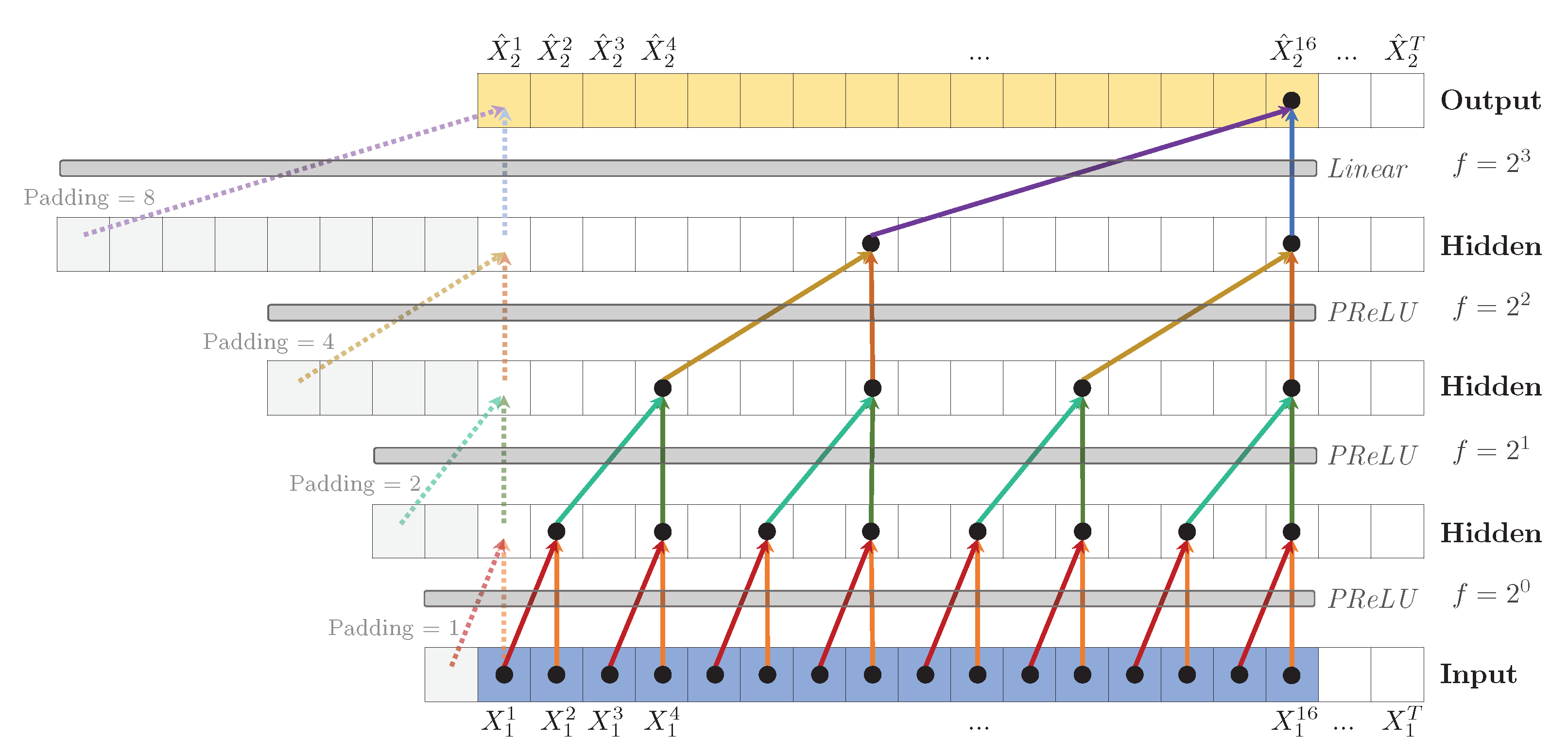
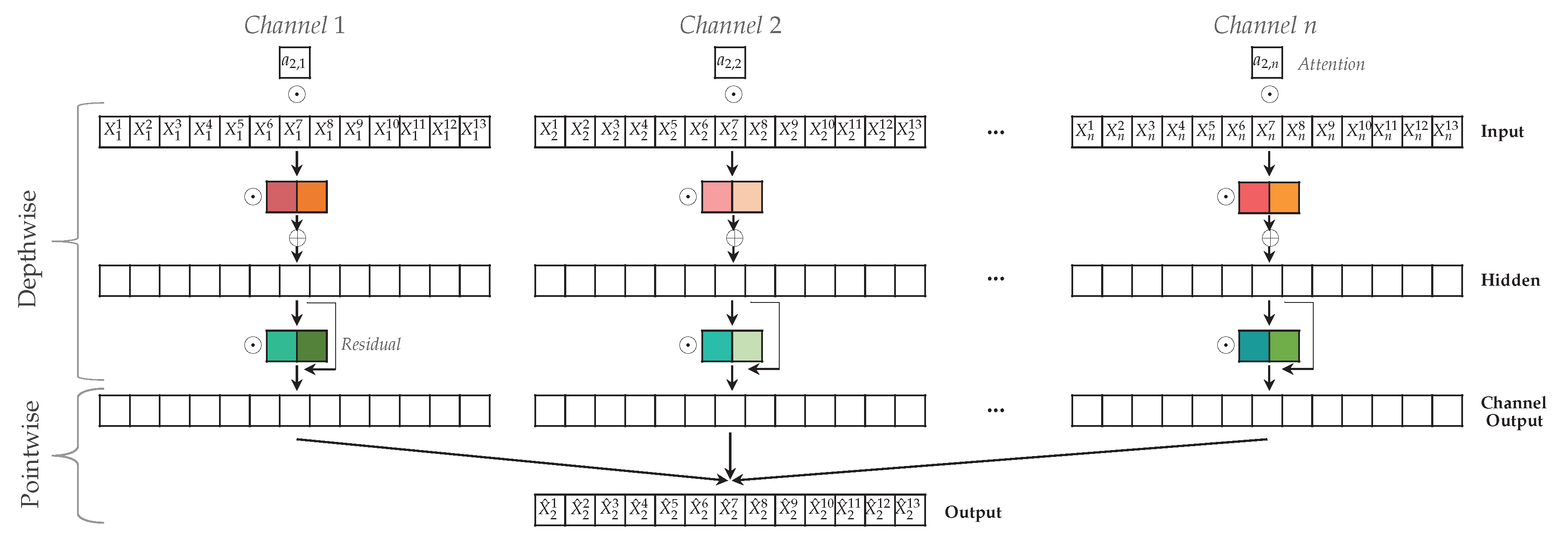
Table 1.
Causal discovery methods for time series data, classified among various dimensions.

Except hidden confounders that are instantaneous and linear [22]. TiMINo stays undecided by not inferring a causal relationship in case of a hidden confounder. Although theoretically shown, the implemented algorithm does not explicitly output the discovered time delays.
Table 2.
Summary of evaluation benchmarks. Delays between cause and effect not available in FMRI.
| FINANCE | FMRI | FMRI | |
|---|---|---|---|
| #datasets | 9 | 27 | 6 |
| #non-stationary datasets | 0 | 1 | 0 |
| #variables (time series) | 25 | {5, 10} | |
| #causal relationships | |||
| time series length | 4000 | 50–5000 (mean: 774) | 1000–5000 (mean: 2867) |
| delays [timesteps] | 1–3 | n.a. | n.a. |
| self-causation | ✓ | ✓ | ✓ |
| confounders | ✓ | ✓ | ✓ |
| type of relationship | linear | non-linear | non-linear |
Table 3.
Time series prediction performance of TCDF, in terms of the mean absolute scaled error (MASE) averaged across all datasets, plus its standard deviation. Best results are highlighted in bold.
Table 3.
Time series prediction performance of TCDF, in terms of the mean absolute scaled error (MASE) averaged across all datasets, plus its standard deviation. Best results are highlighted in bold.
| FINANCE TEST | FMRI TEST | FMRI TEST | |
|---|---|---|---|
| TCDF () | 0.38 ± 0.09 | 0.84 ± 0.38 | 0.71 ± 0.05 |
| TCDF () | 0.38 ± 0.10 | 1.06 ± 0.49 | 0.72 ± 0.07 |
| TCDF () | 0.40 ± 0.10 | 1.13 ± 0.45 | 0.74 ± 0.08 |
Table 4.
Causal discovery overview for all data sets and all methods. Showing macro-averaged F1 and F1’ scores and standard deviations. The highest score per benchmark is highlighted in bold.
Table 4.
Causal discovery overview for all data sets and all methods. Showing macro-averaged F1 and F1’ scores and standard deviations. The highest score per benchmark is highlighted in bold.
| FINANCE (9 Data Sets) | FMRI (27 Data Sets) | FMRI (6 Data Sets) | ||||
|---|---|---|---|---|---|---|
| F1 | F1′ | F1 | F1′ | F1 | F1′ | |
| TCDF () | 0.64 ± 0.06 | 0.77 ± 0.08 | 0.60 ± 0.09 | 0.63 ± 0.09 | 0.68 ± 0.05 | 0.68 ± 0.05 |
| TCDF () | 0.65 ± 0.09 | 0.78 ± 0.10 | 0.58 ± 0.15 | 0.62 ± 0.14 | 0.65 ± 0.13 | 0.68 ± 0.11 |
| TCDF () | 0.64 ± 0.09 | 0.77 ± 0.09 | 0.55 ± 0.13 | 0.63 ± 0.11 | 0.70 ± 0.09 | 0.73 ± 0.08 |
| PCMCI | 0.55 ± 0.22 | 0.56 ± 0.22 | 0.63 ± 0.10 | 0.67 ± 0.11 | 0.67 ± 0.04 | 0.67 ± 0.04 |
| tsFCI | 0.37 ± 0.11 | 0.37 ± 0.12 | 0.49 ± 0.22 | 0.49 ± 0.22 | 0.48 ± 0.28 | 0.48 ± 0.28 |
| TiMINo | 0.13 ± 0.05 | 0.21 ± 0.10 | 0.23 ± 0.12 | 0.37 ± 0.14 | 0.23 ± 0.11 | 0.37 ± 0.15 |
Table 5.
Run time in seconds, averaged over all datasets in the benchmark. TCDF (without parallelism) and TiMINo are run on a Ubuntu 16.04.4 LTS computer with an Intel® Xeon® E5-2683-v4 CPU and NVIDIA TitanX 12GB GPU. PCMCI and tsFCI are run on a Windows 10 1803 computer with an Intel® Core™ i7-5500U CPU.
| TCDF () | PCMCI | tsFCI | TiMINo | |
|---|---|---|---|---|
| FINANCE | 318 s | 10 s | 93 s | 499 s |
| FMRI | 74 s | 1 s | 1 s | 14 s |
Table 6.
Delay discovery overview for all data sets of the FINANCE benchmark (nine datasets). Showing macro-averaged percentage of delays that are correctly discovered w.r.t. the full ground truth, and standard deviation. TiMINo does not discover delays.
Table 6.
Delay discovery overview for all data sets of the FINANCE benchmark (nine datasets). Showing macro-averaged percentage of delays that are correctly discovered w.r.t. the full ground truth, and standard deviation. TiMINo does not discover delays.
| TCDF () | TCDF () | TCDF () | PCMCI | tsFCI | TiMINo | |
|---|---|---|---|---|---|---|
| FINANCE | 97.79% ± 2.56 | 96.42% ± 3.68 | 95.49% ± 4.15 | 100.00% ± 0.00 | 98.77% ± 3.49 | n.a. |
Table 7.
Impact of causal validation step. Showing macro-averaged F1 scores and standard deviation for TCDF with PIVM and TCDF without PIVM. shows the change in F1-score or F1’-score in percent.
Table 7.
Impact of causal validation step. Showing macro-averaged F1 scores and standard deviation for TCDF with PIVM and TCDF without PIVM. shows the change in F1-score or F1’-score in percent.
| FINANCE (9 Data Sets) | FMRI (27 Data Sets) | FMRI (6 Data Sets) | ||||
|---|---|---|---|---|---|---|
| F1 | F1′ | F1 | F1′ | F1 | F1′ | |
| TCDF () | 0.64 ± 0.06 | 0.77 ± 0.08 | 0.60 ± 0.09 | 0.63 ± 0.09 | 0.68 ± 0.05 | 0.68 ± 0.05 |
| TCDF () w/o PIVM | 0.22 ± 0.09 | 0.30 ± 0.13 | 0.60 ± 0.09 | 0.63 ± 0.09 | 0.68 ± 0.05 | 0.68 ± 0.05 |
| (PIVM) | −66% | −61% | 0% | 0% | 0% | 0% |
Table 8.
Results of our TCDF () applied to FINANCE HIDDEN. ‘Equal Delays’ denotes whether the delays from the confounder (conf.) to the confounder’s effects are equal. Grey causal relationships denote that the discovered relationship was not causal according to the ground truth.
Table 8.
Results of our TCDF () applied to FINANCE HIDDEN. ‘Equal Delays’ denotes whether the delays from the confounder (conf.) to the confounder’s effects are equal. Grey causal relationships denote that the discovered relationship was not causal according to the ground truth.
| Dataset | Hidden Conf. | Effects | Equal Delays | Conf. Discovered | Learnt Causal Relationships |
|---|---|---|---|---|---|
| 20-1A | , | ✓ | ✓ | , | |
| 40-1-3 | , | ✓ | ✓ | , | |
| 40-1-3 | , | ✗ | ✗ | ||
| 40-1-3 | , | ✓ | ✓ | , | |
| 40-1-3 | , | ✗ | ✗ | - | |
| 40-1-3 | , | ✗ | ✗ | - | |
| 40-1-3 | , | ✗ | ✗ | - | |
| 40-1-3 | , | ✗ | ✗ | ||
| 40-1-3 | , | ✗ | ✗ | - |
Table 9.
Results of TCDF compared with PCMCI, tsFCI and TiMINo when applied to datasets with hidden confounders. The first row denotes the number of incorrect causal relationships that were discovered between the effects of the hidden confounders. The second row denotes the number of hidden confounders that were located.
| FINANCE HIDDEN | TCDF () | PCMCI | tsFCI | TiMINo |
|---|---|---|---|---|
| # Incorrect Causal Relationships | 2 | 0 | 3 | 8 |
| # Discovered Hidden Confounders | 3 | 0 | 0 | 0 |
© 2019 by the authors. Licensee MDPI, Basel, Switzerland. This article is an open access article distributed under the terms and conditions of the Creative Commons Attribution (CC BY) license (http://creativecommons.org/licenses/by/4.0/).
Share and Cite
MDPI and ACS Style
Nauta, M.; Bucur, D.; Seifert, C. Causal Discovery with Attention-Based Convolutional Neural Networks. Mach. Learn. Knowl. Extr. 2019, 1, 312-340. https://doi.org/10.3390/make1010019
AMA Style
Nauta M, Bucur D, Seifert C. Causal Discovery with Attention-Based Convolutional Neural Networks. Machine Learning and Knowledge Extraction. 2019; 1(1):312-340. https://doi.org/10.3390/make1010019
Chicago/Turabian StyleNauta, Meike, Doina Bucur, and Christin Seifert. 2019. "Causal Discovery with Attention-Based Convolutional Neural Networks" Machine Learning and Knowledge Extraction 1, no. 1: 312-340. https://doi.org/10.3390/make1010019