
NER in Archival Finding Aids: Extended †


Department of Informatics, University of Minho, 4710-057 Braga, Portugal
*
Author to whom correspondence should be addressed.
†
This paper is an extended version of our paper published in SLATE 2021.
Mach. Learn. Knowl. Extr. 2022, 4(1), 42-65; https://doi.org/10.3390/make4010003
Submission received: 1 December 2021
/
Revised: 10 January 2022
/
Accepted: 12 January 2022
/
Published: 17 January 2022
(This article belongs to the Special Issue Language Processing and Knowledge Extraction)
Abstract
:The amount of information preserved in Portuguese archives has increased over the years. These documents represent a national heritage of high importance, as they portray the country’s history. Currently, most Portuguese archives have made their finding aids available to the public in digital format, however, these data do not have any annotation, so it is not always easy to analyze their content. In this work, Named Entity Recognition solutions were created that allow the identification and classification of several named entities from the archival finding aids. These named entities translate into crucial information about their context and, with high confidence results, they can be used for several purposes, for example, the creation of smart browsing tools by using entity linking and record linking techniques. In order to achieve high result scores, we annotated several corpora to train our own Machine Learning algorithms in this context domain. We also used different architectures, such as CNNs, LSTMs, and Maximum Entropy models. Finally, all the created datasets and ML models were made available to the public with a developed web platform, NER@DI.
1. Introduction
Throughout the history of Portugal, there was a need to create an archive where information about the kingdom was recorded.
In 1378, during the reign of D. Fernando, the first known Portuguese certificate was issued by Torre do Tombo (TT), an institution over 600 years old that is still the largest Portuguese archive, storing a significant part of Portuguese historical and administrative records. As time passed, the volume of information contained in national archives has considerably increased, and today there are hundreds of archives spread across the country. Most of them have information from the public administration containing records from the 20th century onwards, however, Portugal has three archives with historical information, the Arquivo Nacional da Torre do Tombo, the Arquivo Distrital da Cidade de Braga, and the Arquivo Distrital da Cidade de Coimbra which record various events throughout the history of the country.
The city of Braga was for many years the administrative capital of northern Portugal and Galicia. In antiquity, most of the records were made by the clergy’s social class. Even today, the church’s strong influence in the district of Braga is still visible, something that influenced the abundance and variety of historical document fonds in the archive of this district.
At the moment, many of these archival documents are already available to the public in digital format, so it is now intended to perform a semantic interpretation of their content. In order to do so, we propose the use of Named Entity Recognition (NER), using Machine Learning (ML), a well-known and widely used technique in Natural Language Processing (NLP). With this approach, we intend to classify and extract different types of Named Entities present in a given archival fond. In this way, several ML algorithms such as Maximum Entropy, Convolutional Neural Networks (CNN), and Recurrent Neural Networks (RNN) will be used to train NER models. Firstly, we accessed several archives’ online repositories and retrieved their archival search aids. Then we generated our own annotated corpora in order to train our models in the archival context. Finally, we validated several models to generate different results and conclude which algorithm best suits the domain and the problem in question.
In the end, a web application was developed where several tools developed in this work, including the ML models, were made available to the public.
2. Related Work
The amount of historical information available in Portuguese archives is increasing, making the exploration of these data complex. The use of the available computational power is not something new for professional historians. In fact, there are several tools that have been developed over time that assist in the archival data processing.
An example of this is the HITEX [1] project, developed by the Arquivo Distrital de Braga between 1989 and 1991. This project consisted of semantic model development for historical archive data, something quite ambitious for the time. Despite this, during its development, it ended up converging to an archival transcription support system, which allowed the transcription of natural text and the annotation by hand of Named Entities, enabling the creation of chronological, toponymic, and anthroponomic indexes.
As for NER, it is a technique that has shown promising results in the last decade. At the moment, there are numerous approaches for extracting information from texts. For example, in [2], this technique was used to extract entities from tweets. In [3], we have another use case of NER, where it was combined with other tools to create a question–answer system. However, most of the experiments in this area were carried out in English. In the Portuguese language, there are fewer works performed in this field. In fact, we only found two annotated datasets available in Portuguese, HAREM and SIGARRA.
HAREM is a NER contest applied to Portuguese text. It had two different events which took place in 2005 [4] and 2008 [5], resulting in two golden collections. In this paper, the second golden collection was used, which consists of a Portuguese annotated corpus that contains about 147,991 words, retrieved from 129 different textual documents, with a total of 7836 manually annotated entities [6]. The textual content of this corpus has been collected from several sources, such as newspapers, web pages, emails, expositories, and political and fiction contexts [7]. As for entity type, ten categories have been annotated: Person, Organization, Time, Place, Works of art, Event, Abstraction, Thing, Value, and Misc.
The other corpus, SIGARRA [8], corresponds to the information system of the University of Porto data. This corpus was created to assist the entity-oriented search engine of the University of Porto; however, an annotated dataset can be used for several Portuguese language NLP tasks. Its content consists of news from 17 organic units from the University of Porto, where a sample with 905 news items was annotated. The identified entities were: Hour, Event, Organization, Course, Person, Location, Date, and Organic Unit. In total, this corpus has a total of 12,644 named entities that were manually annotated.
These datasets have already been used to extract entities from Portuguese texts [9], however, low results were obtained.
3. Named Entity Recognition
One of the objectives of NLP is the classification and extraction of certain entities in textual documents. It is easy to understand that entities, such as people’s names, organizations, places, or dates, translate into crucial information about their contexts. This type of data can be used for various purposes, making this practice very popular. Therefore, a new NLP subfield rises, Named Entity Recognition.
In the past, two different approaches were taken to recognize entities in natural texts. Initially, specific regular expressions were coded to filter various entity types. In some cases, this mechanism delivered good results, mostly when there was an in-depth knowledge of the domain in which this method was intended to be applied. However, this is not always the case. In fact, such an approach was not considered exceptionally dynamic since it is necessary to rewrite a large part of the code if one wants to change the domain language. Furthermore, the existence of ambiguity between entities makes them hard to classify. For example, a person’s name can be used as the name of a place.
Alternatively, statistical classifiers are used. This method consists of using ML models (this paper will deal with supervised ML models [10]) in order to try to predict whether a certain word sequence represents an entity.
This approach has some advantages over the previous one. For example: one can now use this solution in different languages without changing much code; The model can be trained with different parameters and be adjusted to different contexts; An annotated dataset is generated that can be reused for other purposes; etc. In fact, today, several already pre-trained ML models are capable of identifying and classifying various entity types. However, the available models are generic, meaning that the entity prediction for more specific contexts can return results below expectations.
Despite being much more dynamic than the previous approach, using this type of model leads to some work for the experimenter. The experimenter must write down an annotated training dataset to prepare and train the model. Despite being tedious work, it has a low complexity level and therefore does not require great specialization [11].
4. Archival Finding Aids
In this work, we pretend to perform Named Entity Recognition in archival data, more precisely in their descriptions.
Archival search aids, also called archival collection guides or archival descriptions, are documents that describe archival materials. In fact, archival collections can take enormous dimensions, which can make the search for information in these documents extremely challenging. By describing the archive’s content, archival search aids establish administrative, physical and intellectual control over the archives’ holdings, helping the researchers retrieve the information they are looking for much faster.
In Portugal, guidelines for the archival description have been created that describe rules for standardizing the archival search aids. The purpose of these standards is to create a working tool to be used by the Portuguese archivist community in creating descriptions of the documentation and its entity producer. Thus, they promote organization, consistency, and ensure that the created descriptions are in accordance with the associated international standards to this domain. In addition, the adoption of these guidelines makes it possible to simplify the research or information exchange process, whether at the national or international level. These guidelines are divided into three distinct parts:
- Guidelines for descriptions of archival documentation;
- Guidelines for the description of entities holding archival descriptions;
- Guidelines for choosing and building standardized access points.
First, the guidelines for document descriptions consist of creating a solid structure capable of ensuring the consistency and organization of documents, providing methods of retrieving, integrating, sharing, and exchanging data by organizing information through levels of description.
Secondly, there are guidelines for describing archival authorities, which are applied to describe the entities that own or create the archives, for example, individuals, families or even institutions, adding information to contextualize the environment in which the archival documents are created.
Finally, there are guidelines for choosing and building standardized access points. This type of guidance, as its name implies, consists of determining, controlling, and standardizing the method of choosing the access points of the archival documentation, for example, the names of the entities or places associated with the archival documents [12].
In order to process the archival search aids, it is essential to understand its organization, as well as to be aware of its structure. Despite the existence of these standards, they act as guidelines, so it is not always possible to comply with them. It is not expected that these methods will be strictly followed by files documented 500 years ago. In fact, not all organizations have their internal processes structured the same way, so many of the entities that produce archives adopt their own structures, creating mechanisms that satisfy their needs. This can be achieved through the hierarchy system proposed in [12]. In order to create a dynamic mechanism that allows the producing entities to shape the structure of their archival documents according to their own context, a hierarchical system based on levels of description is then used.
- Fond—All archival documents of a given entity or organization constitute a fond;
- Subfond—Corresponds to a subdivision of a fond which can exist independently. For example, administrative departments or family subdivisions;
- Section—A section corresponds to a subset of a fond or subfond which does not have a high degree of autonomy. It may represent geographical, chronological, functional, thematic, or a class of a classification plan. (For many archivists, the concepts of Sub-Fond and Section are equivalent);
- Subsection—Corresponds to a subdivision of a section;
- Series—A series represents a set of documents, simple (pieces) or compound (files), which were associated when they were created because they are documents of a similar nature. Usually, documents belonging to a Series are associated with a specific function or activity or have a common relationship between them;
- Subseries—This level corresponds to a subdivision of a series;
- File—Corresponds to a set of documents organized and grouped for use by its holding entity. Usually, these documents are grouped by some criteria, such as the subject or associated activity;
- Piece or Item—An item corresponds to the simplest element of this system. This can contain the data associated with a letter, images or even sound records;
- Group of Fonds—A group of fonds, as the name implies, corresponds to a set of fonds which are grouped together for some specific purpose, for example, for archival management;
- Collection—The description level Collection corresponds to a set of documents that were grouped in an artificial way through a specific criterion. These documents may belong to different fonds. In addition, a collection can be generated at different levels of description;
- Installation unit—An installation unit corresponds to a structure capable of storing and preserving the desired information. For example, books, notebooks, diskettes, cassettes, databases, etc.
5. OAI-PMH
There are hundreds if not thousands for archives spread across the world. These archives keep records that contain the entire human history, so it is often requested access to their documents. In this way, most archives created their own online repository to allow access to their records. In order to facilitate data sharing, the online repositories use the OAI-PMH (Open Archive Initiative Protocol for Metadata Harvesting) protocol, ensuring the interoperability of standards, promoting broader and more efficient dissemination of information within the archival community. This protocol enables data providers to expose their structured metadata, enabling users to harvest it by using a set of six verbs invoked within HTTP requests [13].
- GetRecord—Verb used to retrieve an individual metadata record from a repository;
- Identify—Verb used to retrieve information about a repository.
- ListIdentifiers—This verb is an abbreviated form of ListRecords, retrieving only headers rather than records;
- ListMetadataFormats—Verb used to retrieve the metadata formats available from a repository;
- ListRecords—Verb is used to harvest records from a repository;
- ListSets—Verb used to retrieve the set structure of a repository.
6. Machine Learning Models
One constraint of extracting entities in archival search aids was obtaining results with high confidence values to use the extracted entities in the future. Thus, we decided to implement several ML approaches to understand which approach would generate better results. In this way, we used three open-source tools that implement different ML algorithms, Maximum Entropy, Convolutional Neural Networks, and Recurrent Neural Networks.
Initially, to train the models to recognize entities in archival search aids, we used two available datasets, HAREM [6] and SIGARRA [8], which contain Portuguese texts with annotated entities. Unfortunately, during validation, we realized that the results obtained did not correspond to the intended ones, which generated the need to create our own annotated corpora in order to train our NER models from scratch.
6.1. OpenNLP
The first tool used to create an ML model was Apache OpenNLP, which consists of a machine learning-based toolkit. Its primary purpose is to perform several Natural language Processing tasks, such as tokenization, sentence segmentation, part-of-speech tagging, named entity extraction, chunking, parsing, and co-reference resolution using ML techniques [14]. In this work, we intend to use only the tokenizer and NER functionalities to process the input data and use it to train an ML model capable of identifying archival search aids named entities. This tool provides pre-trained models in several NLP tasks in several languages such as English, Spanish, Danish, etc., however Portuguese language models are not available for NER. Therefore, in order to use OpenNLP to process Portuguese archival search aids, it is necessary to collect training data and train a new ML model.
The ML architecture used in OpenNLP to perform NER is the Maximum Entropy algorithm, discussed below.
6.1.1. Maximum Entropy
The concept of entropy was introduced by physics thermodynamics, and it was later used in several computer science fields, for example, in the Information Theory and the creation of statistical ML models.
In the Information Theory, the occurrence of a given event with a low probability of occurring translates into more information than the occurrence of an event with a high probability of occurring [15]. In this context, the entropy corresponds to the average quantity of information required to represent an event drawn from the probability distribution for a random variable. In other words, the entropy can be seen as a measure of uncertainty, taking a low value when the probability of certainty for some event is high and a high value when all events are equally likely.
“Information entropy is a measure of the lack of structure or detail in the probability distribution describing your knowledge.”[Jaynes, E.T. 1982]
The concept of entropy was also applied to the statistics field, where it is used to generate statistical models capable of representing real-world problems, usually associated with the prediction of high dimensional data.
Maximum Entropy Models are statistical models that maximize the entropy of probabilistic distribution subjected to an N number of constraints. For that, the first step is to restrict the model to our context domain. This is completed through the creation of features that model our problem. Then, we maximize the entropy of all models that satisfy the previously identified constraints, preventing our model from having features that are not justified by empirical evidence and preserving as much uncertainty as possible [16].
“Ignorance is preferable to error and he is less remote from the truth who believes nothing than he who believes what is wrong.”[Thomas Jefferson (1781)]
6.1.2. Features
To improve our Maximum Entropy model classification, we can classify known information about our concrete problem as constraints. For this, features are used, which consist of binary functions that, for some, give , which represents the class of the entities we are trying to predict, and that represents the possible contexts that we are observing returns the corresponding boolean value. Their function signature is as follows.
Taking this into account, each problem has its own characteristics, which makes it necessary to identify new features when we are faced with different contexts. We can say that features are context-dependent, allowing the algorithm to adapt to different problems. In the function below, an example of a possible feature is represented.
In the Portuguese language, when the token “em” anticipates a word that starts with a capital letter, there is a high probability where that word corresponds to a Place entity type (e.g., “em Lisboa”, “em Inglaterra”). In this way, this feature would help the model to classify Place type entities.
Through this type of constraint, it is possible to restrict the model to our context, however, it is usually necessary to identify more than one feature, which leads to the problem of interdependence between them. This can be resolved iteratively so that the decision to be made, in a given iteration, takes into account previous decisions. This iterative process is really important for sequence tasks, where the previous output can influence the following ones. For example, a person’s name is a sequence of words starting with a capital letter. When the model classifies the first word as a person’s name, there is a high probability that subsequent words starting with a capital letter also belong to that name. Thus, the model must have the ability to consider the decisions previously taken when classifying a certain token.
According to [17], the overlapping feature mechanism is the reason that makes the Maximum Entropy algorithm distinguish itself from other models. It makes it possible to add known information into the model and let the created features overlap to try to predict the best possible outcome.
6.1.3. Entropy Maximization
With all the relevant features identified, we now have to find the best model that satisfies these features to obtain the optimal solution. According to the MaxEnt algorithm, this solution consists of finding the most uncertain distribution subject to the defined constraints to obtain the model that makes the fewest implicit assumptions possible. Thus, the next step is to maximize the entropy of the constrained model.
In order to do so, the function of Information Entropy is used.
This function corresponds to a convex function, in other words, the value of the weighted average of two points is always greater than the value of the function in this set of points. In this way, we can say that the sum of this function is also convex, and when we apply a constraint to this sum, it creates a linear subspace that corresponds to a surface that is also convex. Therefore, the constraint sum has only a global maximum [18]. In the Figure 1 we have an example of the entropy function subjected to restrictions.
According to [19], a constrained optimization problem is required to be solved in order to maximize the entropy of the model subject to a limited number of features. This problem might seem trivial at first glance. In fact, it can even be solved analytically if we have a low number of features; however, if the complexity of the problem increases, i.e., the model has a higher number of overlapping features, it is not possible to find a general solution that way. An alternative to the analytical method is the use of Lagrange Multipliers, forming a Lagrangian function. An example of this resolution can be found in [20].
6.2. spaCy—CNN
The second tool chosen to extract entities from archival search aids was spaCy. Again, this library is equipped with a wide range of NLP tools, NER being one of them. This tool also presents several models pre-trained in texts of various languages, but this time, it also includes the Portuguese language.
Despite having several similarities to OpenNLP, spaCy approaches entity recognition in a very different way, Deep Learning. It is no secret that Neural Networks have unlocked new possibilities in the context of Machine Learning, achieving state-of-the-art results in many fields. That said, we tried to use the Portuguese pre-trained models in the archival context, however, we obtained results below expectations due to the low context proximity, since the spaCy’s pre-trained models were trained in Portuguese news.
Thus, once again, we had to train models from scratch. For this, spaCy implements a mechanism that will be presented below.
6.2.1. Transition Based NER
Sequence tagging tasks such as NER are usually associated with a tagging system that is used to attach a tag to each word of the document we want to classify. However, spaCy uses a transition-based approach to face this problem.
As we can see in Figure 2, this approach is based on transitions between different states in order to correctly classify the target. The general idea about this system is that, given some input token, the model has a set of available actions it can take in order to classify each token, transitioning into the possible state configurations. In the end, the real challenge lies in predicting the actions or transitions to be made to correctly predict the token’s label. To address this challenge, spaCy presents a Deep Learning framework [21].
6.2.2. Deep Learning Framework for NLP
This framework consists of using a statistical model based on Neural Networks to predict the actions to be taken. To apply this principle to natural text, first, we have to process the input tokens calculating representations for the words in the vocabulary. Then, to retain the words’ context, it is necessary to contextualize every token in the sentence, which, in practice, means that we have to recalculate the word’s numeric representation based on the sentence it belongs to. After that, the model comes up with a summary vector, representing all the information needed to help predict the word’s label. With that vector, the model is able to predict the best action to be taken in order to transit to the next state.
In order to simplify this deep learning framework, it can be split into four different steps: Embed, Encode, Attend, and Predict.
6.2.3. Embed
The Embed task, Figure 3, consists of generating numeric representations of each token of the document, the word embeddings. In practice, in this stage, multidimensional vectors for each token are generated in order to create a numeric vocabulary that the model can reason about.
These word embeddings are calculated in order to create a distribution that allows the model to associate words with similar semantic meanings. In other words, tokens that refer to the same entity type will have a similar distribution value. This mechanism provides the model with tools that allow it to have a richer understanding of the vocabulary. For example, given the word “student” in the school context, other words such as “study”, “book”, or “class” are quite likely to be found, because they are all related to the school context. It is important that the information about the words’ proximity is not lost when we create our numeric representations in order to teach the model that those words have some similarity between them. With this embedding mechanism, words such as student, pupil, and finalist will always be very similar in distribution. In this way, these word representations make the model more capable of learning new meanings for words and less limited to his training data.
6.2.4. Encode
In the embedding stage, we created numeric representations for individual tokens, however, the meaning of a word is not always the same and may vary depending on the context where it is inserted. In this way, the Encode task, Figure 4, aims to recalculate the token embeddings, creating context-sensitive vectors.
In order to create context-dependent vectors, we have to recalculate them, taking into account the sentence where they are inserted. A frequent approach to calculate contextualized word vectors in the sentence is the use of RNNs [22] which uses the whole sentence. However, spaCy’s developers believe that using the whole sentence to obtain a word’s context is not the best way to do it. According to them, calculating the word embedding based on the whole sequence will cause the model to have difficulties knowing if a certain context should be associated with the corresponding token. In some cases, this can result in data over-fitting, making the model sensitive to things it should not be sensitive to. Thus, spaCy approaches this problem with CNNs, i.e., with a fixed window of N words for each side of the token, with the belief that in the vast majority of scenarios, a small window of words is all it takes to accurately represent the token’s context.
Furthermore, by using CNNs, one can take advantage of parallelism, which is becoming more and more relevant with the arising of the GPUs’ computational power, something that is not possible with RNNs architectures.
6.2.5. Attend
Now that all the word vectors are contextualized, they can be used to help with the prediction task. The challenge now is to know what information should be taken into account in order to predict the label of a certain word token. For that, spaCy introduces the Attend phase, Figure 5.
This phase consists of selecting all the necessary information in order to correctly classify our target. Given a query vector, the model must come up with relevant data to associate that token to its correspondent entity type.
In order to do so, spaCy utilizes a feature mechanism that dictates the way the output vectors are generated. These features are implemented to help the model find all the word vectors that the query vector attends to. With the defined features, the model should collect all the data needed to classify a certain token. In order to do so, by default, spaCy takes into account the first token in the buffer, the words that are immediately to the left and right of that word, and the last entity previously classified by the model. These features can be defined arbitrarily, ensuring the dynamism and versatility of the model. This allows the experimenter to define new features depending on his own context to fine-tune the model for his domain.
After that, a summary vector is generated that will be used in the prediction phase.
6.2.6. Predict
The last step of this framework consists of the actual prediction of the action that the model should take, given the summary vector generated before.
After all the words are turned into vectors (Embbed), the vectors are contextualized within the sequences (Encode) and the feature defined are taken into account, generating the summary vector (Attend), the system is ready to make the prediction.
In fact, the predict step, Figure 6, consists of taking the resulting vector from the Attend stage and passing it into a simple multi-layer perceptron, which returns the actions probabilities. Then, the model validates all possible actions and chooses one according to the algorithm’s confidence to correctly classify each token of the document.
Finally, this process is iterated through a cycle until the document is finished. It is important to emphasize that all stages of this framework are pre-computed, i.e., they occur outside the cycle, so when the model iterates through the document, fewer computations are needed.
6.3. TensorFlow—RNN
Lately, Deep Learning has been the most used approach to respond to this NLP task. Neural Networks have demonstrated several advances in the NLP field, achieving state-of-the-art results in NER, surpassing previous architectures. In this way, we used Google’s library, TensorFlow, to create an ML model and compare it to the previous tools.
Tensorflow presents several ML features that allow the creation of various Neural Networks architectures. However, this tool is not only applied to NLP tasks, but to any field where the use of Deep Learning is intended. Thus, training a NER model with Tensorflow requires greater knowledge of the entire process involved, from converting vocabulary into word embeddings to training the neural network capable of solving sequence tagging problems.
6.3.1. Recurrent Neural Network
In Deep Learning, the first option that comes to mind when we want to process sequential tasks is the use of RNNs [23]. In NER, the research community started to use these Neural Networks as they revealed pretty good results compared to the existing solutions, making them the standard algorithm for this task.
Despite that, RNNs are also famous for some inconveniences, such as the vanishing gradients making long-term dependencies difficult to deal with. Another problem is that to correctly classify a token’s label, one must consider the word’s neighborhood before and after it. RNNs are unidirectional, which means they can only rely on the prior context of the word, assuming that the model reads the document in linear order. In order to solve some of these problems, new features were added to this algorithm.
6.3.2. Long Short Term Memory
We can think of a Long Short Term Memory (LSMT) as an RNN capable of preserving Long Term Dependencies. In fact, in order to solve the RNN’s memory problem, a memory component was added to it.
This new memory cell keeps a state that is updated across the Neural Network chain by using input, output, and forget gates [24]. In short, these gates are responsible for regulating the data that must be updated at each time-step, the information that must be passed to the next cell and the information that must be forgotten, respectively. Using this mechanism, as we keep updating the memory cell, a notion of context is being created, enforcing the memory capability of an RNN, thus making it more capable of dealing with the Long Term Dependencies problem.
With this solution, the memory problem was attenuated, however the model can still only read the document in one direction, which means that the generated context only refers to the prior words.
6.3.3. Bidirectional Long Short Term Memory
To make the model consider not only the context before the token but also the context after it, a new architecture was used, BI-LSTM.
This new approach consists of processing the document in both directions using two different LSTMs, one for the previous context of the token and another for the subsequent. As we are using LSTMs, this mechanism is capable of keeping long term dependencies, which means that the resulting vector will now have information of the whole sentence. In this way, this approach allows the generation of more robust numeric representations of each token.
Although this approach reveals better results than the use of a simple RNN, it is important to emphasize that a BI-LSTM has a much higher complexity, making the model more difficult to train, needing more time and computational resources.
6.3.4. BI-LSTM-CRF
BI-LSTM came to solve several problems of RNNs, obtaining state-of-art results in several NLP tasks, however, its evolution did not stop there. In fact, in 2015, a new article was released by Huang et al. [25], introducing a new architecture, BI-LSTM-CRF, Figure 7.
This new model consists of adding a Conditional Random Field (CRF) to a BI-LSTM, which enables the model to use sentence-level tag information to help correctly classify the token. Similarly to how BI-LSTM uses past and future features in the prediction task, the CRF layer uses past and future tags to predict the token tag efficiently. In other words, this new component receives the LSTM outputs and is in charge of decoding the best tagging sequence, boosting the tagging accuracy [26].
The use of this architecture has already proved itself, demonstrating state-of-art results in several NLP tasks. In this work, we used the TensorFlow library to implement this algorithm in order to perform NER in archival search aids.
7. Data Processing
In order to train and validate new models capable of recognizing entities in the archival domain, creating annotated data with the respective named entity labels is necessary. In fact, for our ML models to be able to learn how to correctly identify the intended named entities, they need to be trained with numerous data samples. The more representative the examples used, the greater the scope and generalization of the models created. Therefore, training data must be generated from archival context datasets. As we did not find any archival search aids datasets with annotated entities, it was necessary to build our own annotated archival corpora.
In this section, we will cover all the processing of these data, from the harvesting from the archival repositories, annotation, and, finally, the data parse in order to generate the annotated corpora that will be used throughout this work.
7.1. Data Harvesting
The first stage of data treatment was data harvesting. This process consisted of accessing the online repositories of the archives and extracting the intended archival search aids.
In order to do so, the OAI-PMH protocol was used. This protocol allows access to the requested data by using verbs injected in the query string. For example, to extract archival search aids from an archival repository, the following verb can be used: “GetRecord&metadataPrefix=ead&identifier=oai:PT/ABM/:807”. This verb allows us to harvest the archival search aids of the archival fond with reference code “PT/ABM/:807” which, in this case, corresponds to a parish named Paróquia do Curral das Freiras. This specific archival descriptions are kept in the repository of the Arquivo Regional e Biblioteca Pública da Madeira which returns an answer in XML format, containing the metadata regarding the identified fond.
This method was repeated in order to obtain the archival search aids used in this paper.
7.2. Data Description
The data used to test the algorithms referred in this paper correspond to datasets from two national archives: the Arquivo Distrital de Braga (http://pesquisa.adb.uminho.pt (accessed on 15 November 2020)) and the Arquivo Regional e Biblioteca Pública da Madeira (https://arquivo-abm.madeira.gov.pt/ (accessed on 15 November 2020)).
Firstly, there is a dataset of a fond that shows a pioneering period in computing history between 1959 and 1998. This fond (PT/UM-ADB/ASS/IFIP), produced by the International Federation for Information Processing (IFIP), contains a section corresponding to the Technical Committee 2, which has a subsection corresponding to Working Group 2.1. This subsection is composed of several series where different archival descriptions are organized, for example, correspondences, meeting Dossiers, news from newspapers, etc.
Secondly, there are two datasets corresponding to a series (PT/UM-ADB/DIO/MAB/006) from the archival fond Mitra Arquiepiscopal de Braga, which contains genre inquiries. The archival descriptions in this series contain witnesses’ inquiries to prove applicants’ affiliation, reputation, good name or “blood purity”. One of the datasets has a very standardized structure, while the other contains many natural text elements.
Thirdly, there is a historical dataset corresponding to the fond (PT/UM-ADB/FAM/ACA) of the Arquivo da Casa do Avelar (ACA), which depicts the family history of Jácome de Vasconcelos, knight and servant of King D. João I. This family settled in Braga around the years 1396 and 1398 with a total of 19 generational lines, up to the present time. This fond is composed of subfonds and subsubfonds that contain records associated with members of this family with a patrimonial, genealogical and personal domain.
Fourth, there is the dataset of the Familia Araújo de Azevedo (FAA) fond, also known as Arquivo do Conde da Barca. This archive, produced from the year 1489 to the year 1879 by Araújo de Azevedo’s family, who settled in Ponte da Barca and Arcos de Valdevez (district of Viana do Castelo) at the end of the 14th century, contains records predominantly associated with foreign policy and diplomacy across borders. This fond is composed of several subfonds composed of archival descriptions with information from members of the FAA family, such as requirements, letters, royal ordinances, etc.
Fifth, there is a dataset that characterizes the streets of Braga in the year 1750. This corpus contains elements that characterize the history, architecture, and urbanism of each artery in the city, which help to understand the main lines of its evolution.
Finally, two datasets from the Arquivo Regional e Biblioteca Pública da Madeira were used which correspond to two archival fonds, more precisely to Paróquia do Jardim do Mar and Paróquia do Curral das Freiras, both parishes from Madeira archipelago. These fonds consist of three series each, representing registrations of weddings, baptisms, and deaths. Each series consists of files that correspond to the year of each record, and finally, each file has a set of pieces with archival descriptions.
7.3. Data Annotation
In order to perform entity recognition with OpenNLP, spaCy and TensorFlow in these datasets, it is necessary to train different models so that they learn to find Named Entities in different contexts accurately.
For that, it is necessary to have annotated text that represents each dataset domain. In order to do so, a shuffle of each dataset was performed proceeded with the annotation of a significant fraction of each of them. This shuffle allows the data selection to be impartial, making it a more representative sample of each context domain. During the annotation process, several techniques were used, such as regular expressions, manual annotation and even the use of a statistical model proceeded by correction of the output by the annotator. To facilitate this process, a simple JavaScript program was created that allows to annotate texts in the browser with a simple keypress.
In total, the resultant annotated corpora contains 164,478 tokens that make up 6302 phrases where the following named entities types were annotated: Person, Profession or Title, Place, Date, and Organization. All the annotated corpus are available to the public in [27]. The distribution of entities is presented in the Table 1.
7.4. Data Parse
After we have all our datasets annotated, they are ready to be used in the ML model’s training. In this work, different ML toolkits and ML architectures were used, which use different input formats. Thus, it is necessary to perform a data parse for each tool.
7.4.1. OpenNLP Format
In order to train an ML statistical model in the Portuguese archival domain, OpenNLP needs annotations that represent the context in which it will be used to recognize entities. Thus, it is necessary to create data samples in the format presented in Figure 8.
These annotations correspond to real examples of our document annotations. All annotated entities are marked by tags <Start:Entity Type> at the beginning and <END> at the end. It is also interesting to note that the annotations have different types of entities. This is something that was not supported by OpenNLP release versions, however, this feature was later added.
Despite this, writing down just one example is not enough. According to [28], in order to create a NER model that has satisfactory performance with the OpenNLP toolkit, close to 15,000 annotations are needed.
7.4.2. spaCy Format
Another NLP toolkit used to find entities in archival search aids is spaCy, which, like OpenNLP, also requires data samples associated with the archival domain. spaCy accepts new data samples with the format presented in Figure 9.
In this case, we have an example of annotations from the archival search aids of the Arquivo da Casa Avelar archival fond. Here, a python dictionary format was used to annotate the named entities. This dictionary keeps all the token sequences, followed by an array with the entity labels and their delimiting spans, registering the beginning and end of each named entity.
7.4.3. BIO Format
In addition to the NLP toolkits mentioned above in this paper, another Deep Learning architecture was created to recognize entities in this domain, BI-LSTM-CRF. To train this architecture, we used the BIO data format (Beginning, Inside or Outside of the named entity), Figure 10, a common tagging format for tagging tokens, not only in Named Entity Recognition but also in several token level NLP tasks.
These listings correspond to real annotations taken from our annotated archival corpus, archival search aids of the Familia Araujo de Azevedo fond. As we can see, each token is tagged with a label. The label “B-Entity” marks the beginning of the named entity, followed by the label “I-Entity” tagging the token inside of the named entity. All the out of entity tokens are tagged with the label “O”.
7.5. Format Converter
As has already been shown, each of these approaches has a different annotation format, however, the entities annotated are the same. Therefore, in the annotation process, only one format was used to avoid repetition of work. The chosen format was OpenNLP since it was the easiest to manually annotate named entities due to their simple structure. In fact, to annotate an entity in spaCy’s format, we would have to register all the entity spans, making this process slower. As for the BIO, one would have to tokenize and tag each document token, even the Out of Entity tokens which is not optimal. In this way, after having all the data annotated in OpenNLP format, we have to convert it to BIO and spaCy formats. In order to do so, we developed two parsers.
The first one consists of parsing OpenNLP data into spaCy’s format by using regular expressions to find the annotations and determine the entity label, token, and span.
As for parsing the data into the BIO format, we had to tokenize all the sentences into tokens and then tag all the resulting tokens with a BIO label. The way the words are tokenized can affect the model results; therefore, in order to experiment different approaches, three tokenizers were used, Keras API tokenizer, spaCy Portuguese tokenizer, and a simple regex tokenizer. After the tokenization process, we mapped all the entities labels to the new tokenized file. In this way, three versions of the BIO format were created for each dataset. After testing them in the ML models, spaCy’s tokenizer showed better results, probably because it is optimized for the Portuguese language.
8. Models Training
After the annotation process, the annotated datasets were divided into two splits, 70% of each was used to train the models while the remaining 30% was reserved for validation. Then, we feed the training datasets into the ML algorithms in order to train the NER models. In this process, individual optimizations are performed for each tool, such as defining the hyperparameters, tuning the models in order to generate the best results.
8.1. OpenNLP
OpenNLP model’s training process is iterative, so it is necessary to define the number of iterations. It is this iterative process that allows the feature overlap behavior. By default, this hyper-parameter has a value of 100, however, we registered the model results with different number of iterations in order to analyze its behavior.
In Figure 11 we have the learning curves of our model. These learning curves show our model’s training loss and F1-Score (calculated on the evaluation data) by training iteration. As we can see, the loss absolute value is decreasing indefinitely; however, the F1-score rises until iteration 120 and then starts dropping, even with the loss value still decreasing. This means that, after iteration 120, the model starts over-fitting the data, learning the dataset noise. Thus, our final model was trained with 120 iterations.
In addition to the number of iterations, there is yet another parameter to pay attention to, the cut-off. This variable corresponds to the minimum number of times a feature must occur in the model to be considered. In fact, by default, if a feature occurs less than five times, it will not be considered, which helps to reduce noise in the model [11].
8.2. spaCy
For training a NER model with spaCy, we iterated through the data multiple times in order to update its model weights according to the defined spaCy features. By doing so, the model learns how to classify the desired Named Entities. Through these iterations, we calculated the error by comparing the model predictions with the annotated data. However, we do not want the model to overfit the data by memorizing only the given samples. The idea is to create a generalized model capable of performing in new similar contexts across unused data.
In spaCy, this problem is addressed by using the error gradient of the loss function. This mechanism makes the model’s input information less accurate, so it has more difficulties memorizing it. With this approach, spaCy attenuates the data over-fitting problem by passing incomplete data to the model, giving it more freedom in its decisions. Furthermore, this technique is also used to help the model disambiguate words. For example, the word Sameiro may be pre-annotated as a person’s name, however, this word may refer to Santuário do Sameiro, a Portuguese sanctuary. Therefore, the model must be able to discern this situation through the context in which the word is inserted. It must realize what kind of entity a word refers to, based on the words in its neighborhood and not only on the annotated samples. spaCy allows us to set up this dropout mechanism as a customizable hyper-parameter, preventing the model from being limited to the annotated dataset, generalizing it to new contexts [29].
It is important to note that spaCy allows us to use pre-trained word embeddings for multiple languages. In the case of the Portuguese language, spaCy provides a vocabulary with about 500,000 unique vectors trained in datasets, such as [30,31]. In this work we used static embeddings from the model pt_core_news_lg, made available by spaCy. The use of pre-trained embeddings makes the model have a broader knowledge of the vocabulary of the Portuguese language, managing to extract relationships between the words.
Analyzing the Figure 12, at the left side, we can see that the loss of the model decreases over the performed training iterations, increasing its ability to classify the named entities in the training data. On the right side, we have the F1-Score that is calculated on the evaluation data. In fact, the F1-score value increased from iteration 1 to iteration 10, where it peaked. Then, it started to decrease even with the loss value becoming lower. We can say that after iteration 10, the model starts to overfit the training data by learning its noise and putting too much focus on its details. This behavior negatively impacts the performance of the model in unseen data. In this way, spaCy saves the model state of each training iteration in order to select the best model fit at the end of this process.
8.3. TensorFlow BI-LSTM-CRF
In order to train the BI-LSTM-CRF model, we firstly created the data batches, with a max sequence length of 150, using a padding technique. Then, we used the Tensorflow library to implement two LSTMs, one for the forward context and the other for the backwards context. After that, we applied a CRF layer to the LSTMs output in order to process the sequence labels. As for the loss optimizer, we used Adaptive Moment Estimation (Adam), as it helps the model to converge faster and has revealed very good results in several NLP tasks.
This architecture also uses word embeddings, however, they were initialized randomly, with a dimension of 300, and associated with the annotated corpora words. Then, the embedding values were updated in the model’s training so that words with similar meanings would have similar values in distribution.
During the model’s training, we created checkpoints on every 100 training steps. The training and evaluation loss were recorded to generate the Learning Curves of the model.
Observing the Figure 13, the train loss curve (orange) is calculated using the training dataset and helps us to understand how the model is learning. The evaluation loss curve (blue) is calculated with the validation dataset and gives us information about how the model is generalizing.
In this way, we can see that the training curve converges close to the 1200 training steps. As for the evaluation curve, it drops until 1000 training steps and then starts rising indefinitely. This indicates that the model has already learned the training data too well and started over-fitting it. This behavior makes the model learn training data errors or noise too closely and prevents the model from generalizing. In this way, we used the checkpoint model at 1000 training steps for the NER prediction task.
9. Results
The metrics used to measure NER models’ performance are Recall, Precision, and F1-score since the accuracy metric does not satisfy the needs of this NLP field [32].
The main focus of this work was to create a mechanism that could recognize entities from archival search aids with enough confidence. In this way, several NER models were trained with different data contexts. The closer the context of training data and the validation data, the better NER results will be, as the model can rely more on its learning. Thus, in order to test this hypothesis, the first approach consisted of generating individual models for each dataset.
However, even if we can achieve good results within the same corpus, that is not really impressive or useful, as one would have to annotate part of the corpus to extract named entities from it. In this way, the next step was to test the model generalization. In order to do so, we tested how a single model trained with data from all datasets would perform, compared to the last approach. Can the merge of contexts cause the model to become confused? Will it create a more powerful model? In this step, we intended to test those hypotheses. After this, we tested the generalized model with unseen data. In fact, the whole point of generating such a model is to recognize named entities from new data, so it is important to understand how the model will behave in this environment.
9.1. Individual NER Model per Corpus
The first approach of performing NER in archival data was to create one NER model for each annotated corpus from the data processed earlier, splitting the data for training and validation, 70% and 30%, respectively. In this section, we used our OpenNLP, spaCy, and Tensorflow models and presented their validation results.
Looking at the Table 2, we can conclude that the created NER models were able to successfully classify most of the intended entities. It appears that in most cases, the BI-LSTM-CRF model generated with TensorFlow obtains the best results with an F1-score between 86.32% and 100%, followed by spaCy with an F1-score between 70.09% and 100%, and finally OpenNLP with an F1-score between 62.67 and 100%. As we can see with these results, the introduction of Deep Learning on NER reveals significant advances in this field.
It is important to note that only one model was created to validate datasets with high proximity in the context domain, for example, the Inquirições de Genere 2 and Curral das Freiras datasets. As we can see, with the OpenNLP model, when using the corpus Inquirições de Genere 2 to validate the model trained on the Inquirições de Genere 1 dataset, the results obtained were lower (62.67% F1-score) in comparison to the other tools (87.78% and 98.78% F1-score). In this case, it turns out that deep learning has demonstrated a greater capacity for transfer learning.
Finally, analyzing the Table 2 we see that the FAA dataset is the one in which the models presented the lowest results. One reason for this could be that it contains very long sequences. In fact, as previously seen, a Bi-LSTM-CRF is more prepared to deal with Long Term Dependencies, presenting better results than the other tools (86.32% F1-score).
9.2. Generalized NER Model
After obtaining the individual model approach results, an attempt to create a generalized model with annotations from all datasets was made.
Annotating a fraction of a dataset where this technology is to be applied is not always practical, so it would be interesting to create a generalized model capable of adapting to new contexts of similar nature. In fact, by training a model with data from several contexts, it is able to learn more features about the language vocabulary. By doing so, we intend to prepare the model to perform in a wider variety of contexts, which includes text sequences it has never seen. However, this new approach must not obtain worse results than the individual models approach due to the models’ degree of generalization.
For this method, the generalized models were trained with 70% of each dataset to be later validated individually with the remaining 30% of each one.
As can be seen in Table 3, the results obtained by this model are similar to the previous ones, so we can say that the NER performance has not decreased. In this case, the BI-LSTM-CRF model obtained an average of 93.64% F1-Score, followed by the spaCy model with 90.76% F1-score and finally the OpenNLP model with an average of 86.96%.
Now, to measure its performance in a different context, we had to test it with new data. Observing our annotated corpora Table 1, we can see that we did not used one of the annotated corpus in the models’ training. The corpus in question corresponds to the Ruas de Braga dataset, which contains brief notes of the city of Braga streets (the year 1750), with a considerable amount of named entities. We did that to test the performance of the model on an unseen context domain, which is a crucial objective of this NLP task. In the Table 4 we can see the results of this approach.
The results obtained are lower than intended. The best model obtained an F1-score of 68.42, which is low compared to the previous results.
In fact, in addition to the model not having been trained with any part of this dataset, it contains a lot of Organization and Profession type entities. As can be seen in Table 1, the model was trained with few instances of this type, thus their recognition may prove challenging.
On the other hand, it appears that this time, the model generated with BI-LSTM-CRF obtained worse results than the other models. One of the reasons for this could be that this model has a vocabulary restricted to his training data which can lead to a high amount of out of vocabulary words. In fact, both deep learning approaches presented in this paper represent words through word embeddings; however, spaCy uses pre-trained word embeddings from a Portuguese corpus which makes it have a much larger vocabulary. On the other hand, in the BI-LSTM-CRF implementation, we created our own word embeddings during the model’s train, which means that the model only knows the words contained in its training data. In this way, while the spaCy model can assign semantic meaning to words not present in his training data, the BI-LSTM-CRF will identify such words as unknown words, making it hard to reason about them. To conclude, we can say that having a larger vocabulary can become a valuable tool when evaluating corpus with contexts that vary from the model’s training.
10. Web Platform—NER@DI
With the NER models generated, we decided to create a platform in order to make them available to the public. Thus, NER@DI was born, a web platform that provides several tools that were developed throughout this work, such as the annotated corpora, parsers to convert datasets into different formats and, of course, the ML models that make it possible to process archival search aids, extracting relevant named entities.
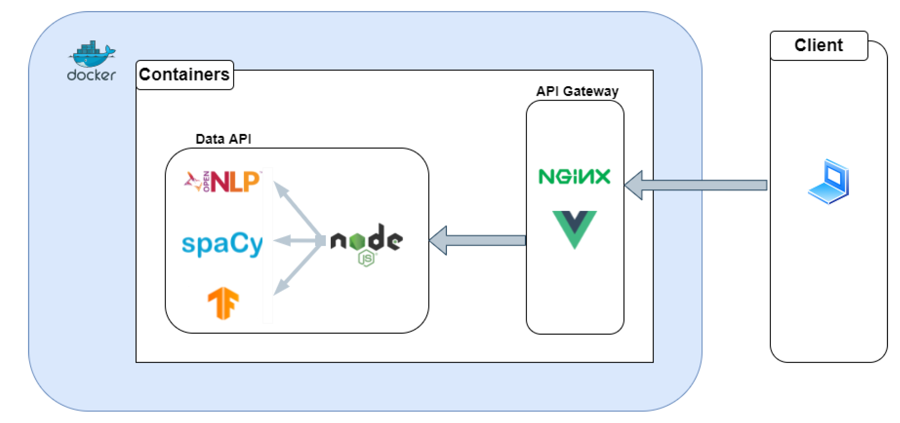
10.1. Architecture
This platform was created with the intent of being complemented with new features in the future. Thus, a micro-service architecture was used, Figure 14, promoting looser coupling, more flexibility and portability.
At the moment, it has two containers that correspond to the Data API and the API Gateway.
The API Gateway is implemented with an Nginx web server containing the client application, developed in Vue.js, a framework that uses reactive interfaces. The use of an API Gateway pattern makes the client less coupled to the micro-services, i.e., it does not need to know the internal structure of the server to communicate with the application. The use of this pattern means that there are no direct references between the client and the microservices, so the refactoring or maintenance of these will not affect the client. On the other hand, if a gateway server was not used, all microservices would be exposed to the public, which could lead to security issues.
Then, Vue.js was used to create the client application. It has a small learning curve, so it is fairly approachable, allowing the creation of maintainable interfaces due to its reusable components mechanism that allows isolating all logic from the views. To complement this framework, Vuetify was used, which consists of a UI library that provides several pre-made reactive components.
The second container is the Data API, which is responsible for receiving, processing, and responding to HTTP requests, in this case, associated with the extraction of entities. For this, a Node.js server was used, complemented by [33] library, which works like a broker that is responsible for managing the API routes and delegating the NER processing to the corresponding tools. The Machine Learning models were implemented with OpenNLP, spaCy, and Tensorflow so, to process NER requests, the Node.js server uses the child_process [34] library, creating new processes to execute programs in python and Java. When the execution of the programs finishes, the created processes return the output to the Node.js server, which is responsible for returning the response to the client in JSON format.
Finally, in order to deploy this platform, each micro-service was wrapped with a docker container. These containers promote the isolation, scalability, agility, and portability of each micro-service since it is really easy to install a containerized application in any system that has docker running. At the moment, NER@DI is hosted on the servers of the University of Minho’s Informatics Department, at [27].
10.2. Features
During this work, several support tools were generated that helped to create and optimize NER’s ML models. Thus, some of these tools were selected to be implemented in NER@DI, presenting the following features:
- Performs Named Entity Recognition with three different ML models, pre-trained in Portuguese archival search aids;
- Implements sorting and filtering functionality that enables, for example, to sort entities by label and remove repeated extracted entities;
- Supports text file import in order to process them with ML models and export the obtained results in CSV and JSON formats;
- Provides tools to parse annotated corpus into different formats, for example, CSV and BIO;
- Provides download methods to all the annotated corpora making it available to the public;
- Presents a set of results from previous entity extractions so that it is possible to verify real case applications of each model in several different corpora.
Thus, NER@DI can be used by various types of users, for example, historians wishing to extract relevant entities from archival documents or even other developers or researchers with the intent of reusing the annotated datasets in other contexts.
11. Conclusions
The main goal of this paper was to create a working tool that was able to recognize entities from archival search aids with enough confidence so the extracted entities could be used in future works. In order to accomplish this, we applied machine learning techniques to a widely used NLP task, NER.
The archival search aids used in this work contain a very specific context, which means that available generic NER models may present lower results than intended. In addition, there is a language barrier, i.e., the amount of Portuguese annotated data available to train this type of model are limited. Despite this, we demonstrated that by training our own models with annotated archival data, it was possible to obtain satisfactory NER results. In fact, with the advances of Deep Learning in this area of NLP, F1-score values above 86% were achieved in almost all of the used datasets.
In the end, we saw that some models performed better than others. In fact, the BI-LSTM-CRF model, trained without pre-trained word embeddings, achieved pretty good results on data with a high degree of similarity with its training data. However, on unseen corpora, it performed poorly. As for the spaCy model, the use of pre-trained word-embeddings demonstrated promising results in unseen contexts managing to achieve the highest results in this scenario.
To conclude, observing the obtained results, it is considered that the use of ML algorithms to perform entity recognition in archival documents, is suitable and with this approach, we can extract information that allows us to create different navigation mechanisms and create relations between information records.
12. Future Work
Several approaches could be put into practice in order to improve the obtained results. For example, we could improve our annotated corpora quantity and quality.
In fact, the corpora used to train the models was not annotated by an archival expert. Some of these documents were written centuries ago, which means that, even if the used language is the same, Portuguese, it is possible that we were not able to identify all the named entities due to vocabulary deviations as a consequence of the language evolution over the years. Because of this, the quality of the annotated data can be negatively affected.
On the other hand, archival documents represent a wide variety of contexts, from documents of public administration, private organizations, religious organizations, etc. In order to create a NER model that can perform in all these different domains, the ML model would need a higher amount of annotated data samples, generating a more representative training environment. This way, it could learn how to classify a broader set of context domains.
As for the actual ML models, it would be interesting to explore new technologies that aim to address this problem, for example, the attention mechanism [35].
Lastly, entity linking could be performed in order to make it possible to browse between different archival documents but related by some entity. It would also be interesting to use the extracted entities to create toponymic and anthroponomic indexes to understand the impact that this tool could have on browsing archival search aids.
Author Contributions
Conceptualization, L.F.d.C.C. and J.C.R.; methodology, L.F.d.C.C. and J.C.R.; software, L.F.d.C.C. and J.C.R.; validation, L.F.d.C.C. and J.C.R.; formal analysis, L.F.d.C.C. and J.C.R.; investigation, L.F.d.C.C. and J.C.R.; resources, J.C.R.; data curation, L.F.d.C.C. and J.C.R.; writing—original draft preparation, L.F.d.C.C. and J.C.R.; writing—review and editing, L.F.d.C.C. and J.C.R.; visualization, L.F.d.C.C. and J.C.R.; supervision, J.C.R.; project administration, J.C.R.; funding acquisition, J.C.R. All authors have read and agreed to the published version of the manuscript.
Funding
This research received no external funding.
Institutional Review Board Statement
Not applicable.
Informed Consent Statement
Not applicable.
Data Availability Statement
The annotated datasets presented in this paper are available at [27].
Conflicts of Interest
The authors declare no conflict of interest.
References
- Oliveira, J.N. HITEX: Um Sistema em Desenvolvimento para Historiadores e Arquivistas. Forum 1992, 23, 127–138. [Google Scholar]
- Derczynski, L.; Maynard, D.; Rizzo, G.; Erp, M.V.; Gorrell, G.; Troncy, R.; Petrak, J.; Bontcheva, K. Analysis of named entity recognition and linking for tweets. Inf. Process. Manag. 2015, 51, 32–49. [Google Scholar] [CrossRef]
- Bellot, P.; Crestan, E.; El-Bèze, M.; Gillard, L.; de Loupy, C. Coupling Named Entity Recognition, Vector-Space Model and Knowledge Bases for TREC 11 Question Answering Track. 2002. Available online: https://citeseerx.ist.psu.edu/viewdoc/download?doi=10.1.1.14.7561&rep=rep1&type=pdf (accessed on 30 November 2021).
- Santos, D.; Seco, N.; Cardoso, N.; Vilela, R. HAREM: An Advanced NER Evaluation Contest for Portuguese. In Proceedings of the Fifth International Conference on Language Resources and Evaluation (LREC’06), Genoa, Italy, 22–28 May 2006; European Language Resources Association (ELRA): Genoa, Italy, 2006. [Google Scholar]
- Freitas, C.; Mota, C.; Santos, D.; Oliveira, H.G.; Carvalho, P. Second HAREM: Advancing the State of the Art of Named Entity Recognition in Portuguese. In Proceedings of the Seventh International Conference on Language Resources and Evaluation (LREC’10), Valletta, Malta, 17–23 May 2010; European Language Resources Association (ELRA): Valletta, Malta, 2010. [Google Scholar]
- Carvalho, P.; Oliveira, H.G.; Santos, D.; Freitas, C.; Mota, C. Segundo HAREM: Modelo geral, novidades e avaliação. 2008. Available online: https://www.researchgate.net/publication/236445432_Segundo_HAREM_Modelo_geral_novidades_e_avaliacao (accessed on 16 November 2020).
- Santos, D.; Cardoso, N. A Golden Resource for Named Entity Recognition in Portuguese. In Computational Processing of the Portuguese Language; Vieira, R., Quaresma, P., Nunes, M.d.G.V., Mamede, N.J., Oliveira, C., Dias, M.C., Eds.; Springer: Berlin/Heidelberg, Germany, 2006; pp. 69–79. [Google Scholar]
- Pires, A.R.O. Named Entity Extraction from Portuguese Web Text. Master’s Thesis, Faculdade de Engenharia da Universidade do Porto, Porto, Portugal, 2017. [Google Scholar]
- Ferreira, J.; Oliveira, H.G.; Rodrigues, R. NLPyPort: Named Entity Recognition with CRF and Rule-Based Relation Extraction. IberLEF@SEPLN. 2019. Available online: http://ceur-ws.org/Vol-2421/NER_Portuguese_paper_7.pdf (accessed on 16 November 2020).
- Sekine, S.; Ranchhod, E. Named Entities: Recognition, Classification and Use; John Benjamins Publishing Company: Amsterdam, The Netherlands, 2009. [Google Scholar]
- Ingersoll, G.S.; Morton, T.S.; Farris, A.L. Taming Text: How to Find, Organize, and Manipulate It; OCLC: ocn772977853; Manning: Shelter Island, NY, USA, 2013. [Google Scholar]
- Rodrigues, A.M.; Guimarães, C.; Barbedo, F.; Santos, G.; Runa, L.; Penteado, P. Orientações para a Descrição Arquivística. 2011. Available online: https://arquivos.dglab.gov.pt/wp-content/uploads/sites/16/2013/10/oda1-2-3.pdf (accessed on 17 October 2020).
- Lagoze, C.; Van de Sompel, H.; Nelson, M.; Warner, S. Open Archives Initiative—Protocol for Metadata Harvesting—V.2.0. 2002. Available online: http://www.openarchives.org/OAI/openarchivesprotocol.html (accessed on 14 October 2020).
- OpenNLP, A. Welcome to Apache OpenNLP. 2017. Available online: https://opennlp.apache.org/ (accessed on 18 October 2020).
- Goodfellow, I.; Bengio, Y.; Courville, A. Deep Learning (Adaptive Computation and Machine Learning Series); The MIT Press: Cambridge, MA, USA, 2016. [Google Scholar]
- Manning, C.D.; Schütze, H. Foundations of Statistical Natural Language Processing; The MIT Press: Cambridge, MA, USA; London, UK, 1999. [Google Scholar]
- Ratnaparkhi, A. Maximum Entropy Models for Natural Language Ambiguity Resolution. Ph.D. Thesis, University of Pennsylva, Philadelphia, PA, USA, 1998. [Google Scholar]
- Manning, C. MaxentModels and Discriminative Estimation. 2003. Available online: https://web.stanford.edu/class/cs124/lec/Maximum_Entropy_Classifiers.pdf (accessed on 22 January 2021).
- Berger, A.L.; Della Pietra, V.J.; Della Pietra, S.A. A Maximum Entropy Approach to Natural Language Processing. Comput. Linguist. 1996, 22, 39–71. [Google Scholar]
- Morais, M. NEU 560: Statistical Modeling and Analysis of Neural Data: Lecture 8: Information Theory and Maximum Entropy. 2018. Available online: http://pillowlab.princeton.edu/teaching/statneuro2018/slides/notes08_infotheory.pdf (accessed on 20 October 2020).
- spaCy. Model Architecture. 2017. Available online: https://spacy.io/models (accessed on 14 January 2021).
- Lample, G.; Ballesteros, M.; Subramanian, S.; Kawakami, K.; Dyer, C. Neural architectures for named entity recognition. In Proceedings of the 2016 Conference of the North American Chapter of the Association for Computational Linguistics: Human Language Technologies, NAACL HLT 2016, San Diego, CA, USA, 12–17 June 2016. [Google Scholar] [CrossRef]
- Graves, A.; Mohamed, A.R.; Hinton, G. Speech recognition with deep recurrent neural networks. In Proceedings of the ICASSP, IEEE International Conference on Acoustics, Speech and Signal Processing—Proceedings, Vancouver, BC, Canada, 26–31 May 2013. [Google Scholar] [CrossRef] [Green Version]
- Olah, C. Understanding Lstm Networks. 2015. Available online: http://colah.github.io/posts/2015-08-Understanding-LSTMs (accessed on 10 March 2021).
- Huang, Z.; Xu, W.; Yu, K. Bidirectional LSTM-CRF Models for Sequence Tagging. arXiv 2015, arXiv:1508.01991. [Google Scholar]
- Ma, X.; Hovy, E. End-to-end sequence labeling via bi-directional LSTM-CNNs-CRF. In Proceedings of the 54th Annual Meeting of the Association for Computational Linguistics, ACL 2016—Long Papers, Berlin, Germany, 7–12 August 2016. [Google Scholar] [CrossRef] [Green Version]
- Cunha, L.F.; Ramalho, J.C. NER@DI. 2021. Available online: http://ner.epl.di.uminho.pt (accessed on 9 October 2021).
- Community, A.O.D. Apache OpenNLP Developer Documentation. 2011. Available online: https://opennlp.apache.org/docs/1.8.2/manual/opennlp (accessed on 10 April 2021).
- spaCy. Training spaCy’s Statistical Models · spaCy Usage Documentation. Available online: https://spacy.io/usage/training (accessed on 14 January 2021).
- Rademaker, A.; Chalub, F.; Real, L.; Freitas, C.; Bick, E.; de Paiva, V. Universal Dependencies for Portuguese. In Proceedings of the Fourth International Conference on Dependency Linguistics (Depling), Pisa, Italy, 18–20 September 2017; pp. 197–206. [Google Scholar]
- Nothman, J.; Ringland, N.; Radford, W.; Murphy, T.; Curran, J.R. Learning multilingual named entity recognition from Wikipedia. Artif. Intell. 2017, 194, 151–175. [Google Scholar] [CrossRef] [Green Version]
- Derczynski, L. Complementarity, F-score, and NLP evaluation. In Proceedings of the 10th International Conference on Language Resources and Evaluation, LREC 2016, Portorož, Slovenia, 23–28 May 2016. [Google Scholar]
- Express—Node.js Web Application Framework, n.d. Available online: https://expressjs.com (accessed on 10 April 2021).
- Node.js v16.4.0 Documentation, n.d. Available online: https://nodejs.org/api/child_process.html (accessed on 17 March 2021).
- Vaswani, A.; Shazeer, N.; Parmar, N.; Uszkoreit, J.; Jones, L.; Gomez, A.N.; Łukasz, K.; Polosukhin, I. Attention Is All You Need. 2017. Volume 2017-December. Available online: https://arxiv.org/abs/1706.03762 (accessed on 11 September 2021).
Figure 1.
Entropy function subject to restrictions.

Figure 2.
Example of transition based sequence applied on NER.

Figure 3.
Embed process.

Figure 4.
Encode process.

Figure 5.
Attend process.

Figure 6.
Predict process.

Figure 7.
Bidirectional Long Short Term Memory Conditional Random Field.

Figure 8.
OpenNLP annotation from the Família Araújo de Azevedo corpus.

Figure 9.
spaCy annotations from Arquivo da Casa Avelar corpus.

Figure 10.
BIO annotation from the Família Araújo de Azevedo corpus.

Figure 11.
OpenNLP model learning curves.

Figure 12.
spaCy model learning curve.

Figure 13.
BI-LSTM-CRF model learning curve.

Figure 14.
NER@DI architecture.


Table 1.
Number of annotated entities per corpus.
| Corpus | Person | Place | Date | Profession or Title | Organization | Total |
|---|---|---|---|---|---|---|
| IFIP | 1503 | 325 | 100 | 40 | 318 | 2286 |
| Familia Araújo de Azevedo | 369 | 450 | 118 | 428 | 94 | 1459 |
| Arquivo da Casa Avelar | 465 | 239 | 141 | 118 | 91 | 1054 |
| Inquirições de Genere 1 | 2002 | 3713 | 121 | 0 | 0 | 5836 |
| Inquirições de Genere 2 | 692 | 10 | 54 | 0 | 0 | 756 |
| Jardim do Mar | 2393 | 574 | 1762 | 1 | 2 | 4732 |
| Curral das Freiras | 8729 | 0 | 0 | 0 | 0 | 8729 |
| Ruas de Braga | 1126 | 1293 | 684 | 391 | 338 | 3832 |
| Total | 17,279 | 6604 | 2980 | 978 | 843 | 28,684 |
Table 2.
Individual NER models results.
| Train | Validation | Tool | Precision (%) | Recall (%) | F1-Score (%) |
|---|---|---|---|---|---|
| IFIP | IFIP | OpenNLP | 87.08 | 82.61 | 84.79 |
| spaCy | 88.16 | 89.90 | 89.02 | ||
| BI-LSTM-CRF | 96.12 | 98.67 | 97.00 | ||
| Familia Araújo de Azevedo | Familia Araújo de Azevedo | OpenNLP | 72.56 | 72.30 | 72.43 |
| spaCy | 74.41 | 72.82 | 74.09 | ||
| BI-LSTM-CRF | 88.98 | 87.28 | 86.32 | ||
| Arquivo da Casa Avelar | Arquivo da Casa Avelar | OpenNLP | 80.15 | 79.85 | 80.00 |
| spaCy | 87.82 | 87.18 | 87.50 | ||
| BI-LSTM-CRF | 89.25 | 93.25 | 90.63 | ||
| Inquirições de Genere 1 | Inquirições de Genere 1 | OpenNLP | 99.93 | 98.87 | 99.90 |
| spaCy | 97.35 | 95.08 | 96.20 | ||
| BI-LSTM-CRF | 100 | 100 | 100 | ||
| Inquirições de Genere 1 | Inquirições de Genere 2 | OpenNLP | 63.17 | 62.17 | 62.67 |
| spaCy | 89.66 | 85.98 | 87.78 | ||
| BI-LSTM-CRF | 98.86 | 98.95 | 98.78 | ||
| Jadim do Mar | Jardim do Mar | OpenNLP | 100 | 99.86 | 99.93 |
| spaCy | 100 | 100 | 100 | ||
| BI-LSTM-CRF | 100 | 100 | 100 | ||
| Jadim do Mar | Curral das Freiras | OpenNLP | 93.37 | 99.84 | 96.50 |
| spaCy | 99.97 | 99.90 | 99.93 | ||
| BI-LSTM-CRF | 100 | 100 | 100 |
Table 3.
Generalized NER model validation results.
| Corpus | Model | Precision (%) | Recall (%) | F1-Score (%) |
|---|---|---|---|---|
| IFIP | OpenNLP | 89.43 | 83.60 | 86.41 |
| spaCy | 86.99 | 88.71 | 87.84 | |
| BI-LSTM-CRF | 92.84 | 96.85 | 94.08 | |
| Família Araújo Azevedo | OpenNLP | 81.94 | 63.67 | 71.66 |
| spaCy | 75.19 | 76.78 | 75.98 | |
| BI-LSTM-CRF | 78.22 | 82.47 | 78.89 | |
| Arquivo da Casa Avelar | OpenNLP | 88.84 | 81.68 | 85.11 |
| spaCy | 87.18 | 87.18 | 87.18 | |
| BI-LSTM-CRF | 86.83 | 92.21 | 87.99 | |
| Inquirições de Genere 1 | OpenNLP | 99.60 | 99.53 | 99.57 |
| spaCy | 98.31 | 96.74 | 97.52 | |
| BI-LSTM-CRF | 100 | 100 | 100 | |
| Inquirições de Genere 2 | OpenNLP | 74.70 | 65.61 | 69,80 |
| spaCy | 79.96 | 92.21 | 87.26 | |
| BI-LSTM-CRF | 93.70 | 98.34 | 94,82 | |
| Jardim do Mar | OpenNLP | 99.71 | 99.71 | 99.71 |
| spaCy | 99.15 | 100 | 99.57 | |
| BI-LSTM-CRF | 100 | 99.60 | 99.72 | |
| Curral das Freiras | OpenNLP | 93.49 | 99.69 | 96.49 |
| spaCy | 99.98 | 99.90 | 99.94 | |
| BI-LSTM-CRF | 100 | 100 | 100 |
Table 4.
Generalized NER model validation results on Ruas de Braga corpus.
| Corpus | Model | Precision (%) | Recall (%) | F1-Score (%) |
|---|---|---|---|---|
| Ruas de Braga | OpenNLP | 73.09 | 61.09 | 66.55 |
| spaCy | 75.39 | 62.62 | 68.42 | |
| BI-LSTM-CRF | 50.50 | 58.80 | 53.00 |
Publisher’s Note: MDPI stays neutral with regard to jurisdictional claims in published maps and institutional affiliations. |
© 2022 by the authors. Licensee MDPI, Basel, Switzerland. This article is an open access article distributed under the terms and conditions of the Creative Commons Attribution (CC BY) license (https://creativecommons.org/licenses/by/4.0/).
Share and Cite
MDPI and ACS Style
Cunha, L.F.d.C.; Ramalho, J.C. NER in Archival Finding Aids: Extended. Mach. Learn. Knowl. Extr. 2022, 4, 42-65. https://doi.org/10.3390/make4010003
AMA Style
Cunha LFdC, Ramalho JC. NER in Archival Finding Aids: Extended. Machine Learning and Knowledge Extraction. 2022; 4(1):42-65. https://doi.org/10.3390/make4010003
Chicago/Turabian StyleCunha, Luís Filipe da Costa, and José Carlos Ramalho. 2022. "NER in Archival Finding Aids: Extended" Machine Learning and Knowledge Extraction 4, no. 1: 42-65. https://doi.org/10.3390/make4010003