Spinning Reserve Capacity Optimization of a Power System When Considering Wind Speed Correlation

1
Control Engineering College, Chengdu University of Information Technology, Chengdu 610225, Sichuan Province, China
2
Kills Training Center of State Grid Sichuan Electric Power Corporation, Chengdu 610031, Sichuan Province, China
3
Department of Electrical Engineering, Henan polytechnic, Zhengzhou 450046, Henan Province, China
*
Author to whom correspondence should be addressed.
Appl. Syst. Innov. 2018, 1(3), 21; https://doi.org/10.3390/asi1030021
Submission received: 1 May 2018
/
Revised: 21 June 2018
/
Accepted: 21 June 2018
/
Published: 26 June 2018
Abstract
:Usually, the optimal spinning reserve is studied by considering the balance between the economy and reliability of a power system. However, the uncertainties from the errors of load and wind power output forecasting have seldom been considered. In this paper, the optimal spinning reserve capacity of a power grid considering the wind speed correlation is investigated by Nataf transformation. According to the cost–benefit analysis method, the objective function for describing the optimal spinning reserve capacity is established, which considers the power cost, reserve cost, and expected cost of power outages. The model was solved by the quantum-behaved particle swarm optimization (QPSO) algorithm, based on stochastic simulation. Furthermore, the impact of the related factors on the optimal spinning reserve capacity is analyzed by a test system. From the simulation results, the model and algorithm are proved to be feasible. The method provided in this paper offers a useful tool for the dispatcher when increasing wind energy is integrated into power systems.
1. Introduction
Wind power, which is a green, clean, and renewable energy source, has developed dramatically. Unlike traditional power sources, wind energy in a power system has the following characteristics: (1) the intermittent and variable nature of wind speed causes the output power of wind farms to be stochastic; (2) as wind farms are commonly clustered in a region rich in wind resources, wind speeds and wind speed forecast errors of different wind farms are dependent. As wind power cannot be predicted with great accuracy, additional spinning reserve needs to be carried in order to guarantee the operational reliability [1]. Therefore, it is of great significance that new spinning reserve dispatch methods capable of taking account into probabilistic and correlated characteristics of wind power are developed.
There have been many studies on the spinning reserve of power grids with large-scale wind power. Zhang, et al. [2] and Zhang, et al. [3] set up deterministic optimization modes for spinning reserve capacity, where the objective function is the minimum cost to buy spinning reserve. In [4], the system states are quickly selected by using the enumeration and simulation method, and a new method is used to assess the operating reserve risk of the wind power system. An optimization algorithm for the spin reserve is presented in [5] for the different demand of spin reserves under risk, using the control performance of the generator set. However, the relationship between the abundant levels of spinning reserves and the reliability and economy of the power grid is not well considered. In [6], a model of the generation and optimal coordinating dispatch reserves is built, in which the constraint condition of the quantitative relation of the ratio between the system reserves and expected loss of load is considered. Taking both system economy and reliability into consideration, Literature [7] propose a conditional value-at-risk-based optimal spinning reserve model and incorporate it into the generation scheduling model in wind power integrated systems, in order to minimize total generation cost. Considering uncertainties in wind power and load forecasts, a multi-objective energy and spinning reserve scheduling method for a wind–thermal power system is investigated in a market environment [8]. Cobos, et al. [9] establishes a mathematical optimization model for the minimum cost of conventional generators and spinning reserve, and then adopts a robust linear optimization to get the optimal reserve capacity with the wind uncertainty, so as to guarantee the feasibility of the optional solutions for all the realizations of the uncertain data. In [10], based on a robust optimization approach, an energy and reserve joint dispatch model in the real-time electricity markets is presented, considering wind power generation uncertainties as well as zonal reserve constraints under both normal and N-1 contingency conditions.
However, the above references have not considered the influence of wind speed correlation on the spinning reserve capacity. Li, et al. [11], Chen, et al. [12], and Xie and Xiong [13] take into account the wind speed correlation to investigate optimal power flow, reliability assessment, and dynamic economic dispatch of power systems with integrated wind power, respectively. These studies have shown wind speed correlation should not be neglected when several wind farms are connected to the same power system.
In this paper, a stochastic spinning reserve capacity optimization model is set up, taking account into the wind speed correlation and some uncertain factors. Compared with the prior works, the major contributions of this paper are summarized as:
- (1)
- The wind speed correlation is considered. The Nataf transformation and Cholesky decomposition are applied to model the correlated wind speed;
- (2)
- An optimal spinning reserve model is proposed, aiming at the minimum generator cost, spinning reserve cost, and expected outage cost, in which the other uncertain factors, such as the load forecast deviation, wind power output prediction error, and forced outage rate of the generator are all considered;
- (3)
- The model is solved by the quantum-behaved particle swarm optimization (QPSO), based on the stochastic simulation algorithm.
The rest of the paper is organized as follows. Section 2 addresses the modeling method of wind speed correlation. Section 3 presents the optimization model of spinning reserve capacity. Section 4 employs the stochastic optimization algorithm, QPSO, to solve the model. In Section 5, tests and comparisons under different wind speed correlations are demonstrated. Finally, conclusions are drawn in Section 6.
2. The Model of Correlated Wind Speeds
2.1. Nataf Transformation
The Nataf transformation and Cholesky decomposition are used to convert non-normal relevant variables to independent standard normal ones.
For the input speed wind vector , whose probability density function (PDF) and marginal cumulative distribution function (CDF) are known, using marginal transformations, Liu and Der [14] obtained the jointly standard normal variate vector , which is expressed as:
where is the CDF of standard normal variable (SNV), and is the inverse CDF of SNV.
The relationship between correlation coefficient ρij of vector V and correlation coefficient ρ0,ij of vector X can be expressed as
where ρij of ρ0,ij of are, respectively, the elements of correlation matrix ρ of vector V and the ρ0 of vector X, μi and σi are the mean and standard deviation of wind speed vi, respectively; is the bi-dimensional standard normal PDF of zero means, unit standard deviations, and correlation coefficient ρ0,ij.
In most engineering applications, ρ0 is a positive definite, so it can be decomposed by Cholesky decomposition.
where L0 is an inferior triangular matrix.
Then, the correlated standard norm vector X is transformed into an independent standard normal vector by using L0.
Through Equations (1)–(4) above, the correlated non-normal wind speed vector V is transformed to the independent standard normal vector U, and this is the positive process of Nataf transformation.
2.2. The Solution for the Correlation Coefficient of the Wind Speed
For the complexity of calculating Equation (2), Dagang [15] employed the integral space transformation method to transform Equation (2) into Formula (5), as follows:
where ui, uj is the ith and jth element of the vector U, respectively, and is the PDF.
Then, the bi-dimensional Nataf transform and Gauss–Hermite integral method are applied to calculate the integral in Formula (5), can be achieved by solving the nonlinear equation as follows:
where m is the number of integral nodes; wl and wk are the weight values of the integral nodes l and k, respectively; and is derived from Equations (7) and (8), as follows:
where is a bi-dimensional inferior triangular decomposition matrix, which is derived from Nataf transformation; ; and the typical weight values wl and wk and the node values zil and zjk can be obtained from the literature [16].
2.3. Generation of the Random Numbers of Correlated Wind Speeds
When CDFs F(V) and correlation matrix ρ of correlated wind speeds are available, the random numbers of wind speeds can be generated by inverse Nataf transformation. The basic steps are as follows:
- (1)
- Generate the random numbers Us of vector U;
- (2)
- Achieve the correlation matrix ρ0 of the correlated standard norm vector X by Equations (6)–(8), then ρ0 is decomposed by Cholesky decomposition to get the matrix L0;
- (3)
- Generate the random numbers Xs of vector X by Equation (4);
- (4)
- Generate the correlated random numbers Vs of wind speed vector V by marginal transformation.
3. Optimization Model
3.1. Objective Function
According to the cost–benefit analysis method, an objective function is built as the following, which is the minimum cost containing the generation cost, reserve cost, and expected outage cost.
where N is the number of thermal power units; T is the number of the scheduling interval; f(pi,j) is the cost of thermal power generator unit i at the time t, which includes the operating cost and start-up fee Si,t; ai, bi, and ci are the cost coefficients of the generator unit i; Pi,t is the output of thermal power unit i at the time t; g(ri,j)is the reserve cost; αi,u is the up spinning reserve price of the unit; αi,d is the down spinning reserve price of the unit i; ru,i,t and rd,i,t are the up and down spinning reserve capacities, respectively; Ot is the expected outage cost; γ is the power loss cost, which can be obtained from statistical results; Et is the expected energy not serve (EENS) of the power system at the time t, which can be calculated by
where y is the electricity demand deviation of the whole power system, Mr is the up spinning reserve capacity at the time t, ΔPg is the dispatching difference of the thermal power units due to outage, and f(y) is PDF of the electricity demand deviation y.
3.2. Constraints
Constraint conditions mainly include the power balance (Equation (15)), the generation limits (Equation (16)), minimum running time (Equation (17)), outage time constraints (Equation (18)), and ramping constraints (Equation (19)), which are defined as follows:
where S is the number of wind farms, is the power output of the jth wind farm at the time t; is the load power at t; and are the minimum and maximum available power output of thermal power unit i at t, respectively; and are the operation and shutdown time, respectively, of the unit i at t; and are the minimum values of operation time and shutdown time, respectively; and are the ramp-down and the ramp-up limit of the thermal power generator i, respectively.
Due to the random and fluctuation of the wind power outputs and loads, some additional constraint conditions should be considered. In this paper, the probability intervals of the wind power and loads are both set as 95%, which are respectively defined as and . Furthermore, the up and down spinning reserve capacities and needed to supply the power system at t are as follows:
The up and down spinning reserve constraints of the thermal power unit are as follows:
where ri,u and ri,d are the up and down spinning reserve capacity supplied by the thermal power generator unit i, respectively; β is the confidence level of the system; di,t is the state variable of the thermal power generator unit i, and di,t = 0 when the unit i is not scheduled to run in the day-ahead dispatch. Otherwise, di,t is determined by the forced outage rate qi of the unit i by Monte Carlo stochastic simulation: randomly generate a pseudo-random number δi following the uniform distribution [0,1], if , di,t = 0, otherwise, di,t = 1.
3.3. The Prediction Deviation
In a power system that includes wind farms, the prediction deviation is mainly from the load forecast error and the prediction error of the wind farm output. Firstly, the load forecast deviation is as follows:
where is the forecast load and is the load forecast deviation, which follows the normal distribution .
The wind farm output prediction deviation is
where and are the actual and forecast values of wind farm output, respectively, and is the wind power output prediction deviation, which follows the normal distribution . The standard prediction deviation at the time t can be calculated as
where K is the factor of wind power prediction error and WI is the total installed capacity of the wind farms.
The actual electric demand of the power system can be calculated as
where PQ,t is the electric demand forecast of the whole power system, and ΔPQ,t is the electric demand deviation of the whole power system, which is assumed to follow the normal distribution . The standard deviation at the time t is
According to the Wang, et al. [17], the continuous probability density function of the electric demand deviation is defined as
4. Solution Algorithm
The QPSO has many advantages [18], such as global convergence, faster convergence speed, fewer control parameters, and powerful search abilitities, so the QPSO based on the stochastic simulation algorithm is applied to solve the optimization model in this paper.
4.1. Stochastic Simulation
The procedure of the stochastic simulation is as follows:
- (1)
- Set the counter to N’ = 0;
- (2)
- Randomly generate the variable samples of the thermal power output and reserve capacity, then substitute them into Formulas (23) and (24) to test the feasibility of these samples—if they satisfy (23) and (24), then ;
- (3)
- Repeat Step 2 above for N times, until N′/N > β.
4.2. Quantum-Behaved Particle Swarm Optimization
The QPSO is a probability search algorithm that introduces quantum mechanics into particle swarm optimization (PSO). The average best position C(k) is introduced into QPSO to calculate variables in the following iteration:
where M is the number of the swarm, k is the current number of iterations, and pi is the local best position of the swarm i.
The particle position of decision variables xi is updated through the Monte Carlo stochastic simulation, as follows:
where u is uniform random numbers in the interval [0,1], and λ is the contraction–expansion coefficient, which can be applied to control the convergence speed of PSO algorithm. The contraction–expansion coefficient is defined as
where Maxiter is the maximum number of the inner iterations.
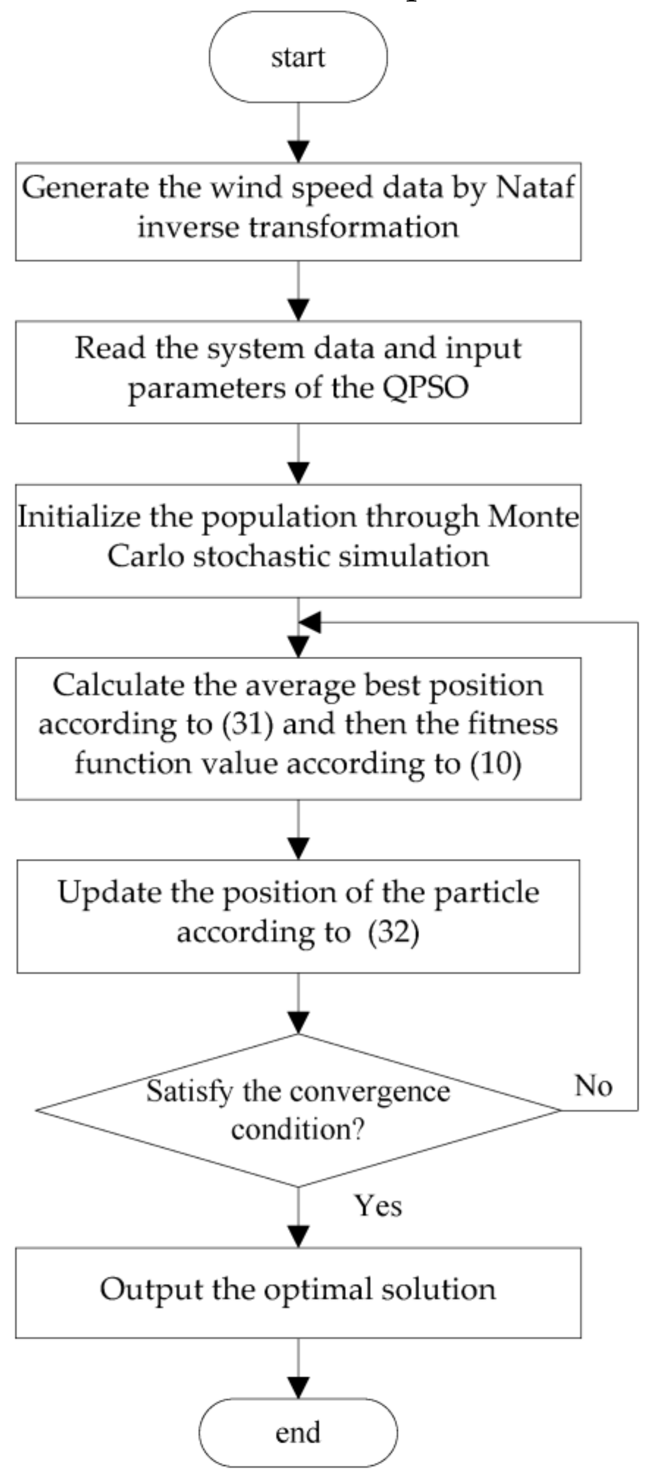
The flow chart of the proposed QPSO based on Equations (31)–(33) is shown as Figure 1.
The detailed procedure is as follows:
- (1)
- Obtain the correlated wind speed data of wind farms, according to Section 2.3;
- (2)
- Read the system data, such as the prediction values of the loads and wind power output and the probability distribution of the prediction deviation. In addition, set the input the parameters of the quantum-behaved particle swarm optimization algorithm, such as maximum iteration number and particle swarm size;
- (3)
- Initialize the population. The active power and reserve capacity of each thermal power unit are randomly generated to form the population, which is tested according to Formulas (15)–(24); if the population is not feasible, it will be regenerated until Formulas (15)–(24) are satisfied;
- (4)
- Calculate the average best position of the particle swarm, according to Formula (31), and then calculate the fitness function value of particles at the current location according to Formula (10);
- (5)
- Update the position of the particles. The position of each particle is updated according to Formula (32), and the limit is verified. If the decision variables are beyond their limits, the particles are renewed. Besides, a random simulation is also employed to verify whether the particles are satisfied with the predetermined confidence level, and if they do not satisfy the confidence level, the particles will be renewed. Then the fitness function values of each particle are calculated. If they are superior to the extreme value of the current particles, the individual extremum is updated. If the individual extreme value of the population is better than the current global extreme value, then update the global optimum;
- (6)
- Determine whether the convergence condition is satisfied, or if the number of iterations is reached. If it is not satisfied, then go back to Step 4—otherwise, output the best particle as the optimal solution.
5. Analysis of Examples
5.1. Parameter Configuration
In this paper, the test system consists of 16 thermal power units and four wind farms. The basic data are listed in Table A1 and Table A2 in Appendix A. The relationship between the wind farm power and the wind speed is as follows:
where Pr is the rated power of a wind farm; υci, υr, and υout are the cut-in speed, rated speed, and cut-out speed, which are 3, 12, and 20 m/s, respectively for all wind farms. Load forecast deviation obeys the normal distribution N(0, 202). The wind power prediction error factor is 0.02. The loss value for outage is 500 USD/MW·h. In QPSO, the number of swarms is 40, and the maximum number of iterations is 500, the parameter = 1 × 10⁻⁴.
5.2. Nataf Transformation
The wind speed distribution for every wind farm is assumed to follow the Weibull distribution, in which the scale and shape parameters are 8 m/s and 2.2, respectively. All four wind farms are correlated with correlation coefficient ρ, and the correlation coefficient matrix is defined as
For the strong positive correlation, moderate correlation, low correlation, and negative correlation, the correlation coefficients are set as 0.9, 0.5, 0.1, and −0.5, respectively. In this paper, five integral nodes are selected to solve the correlation coefficient ρ0, which are listed it in Table 1.
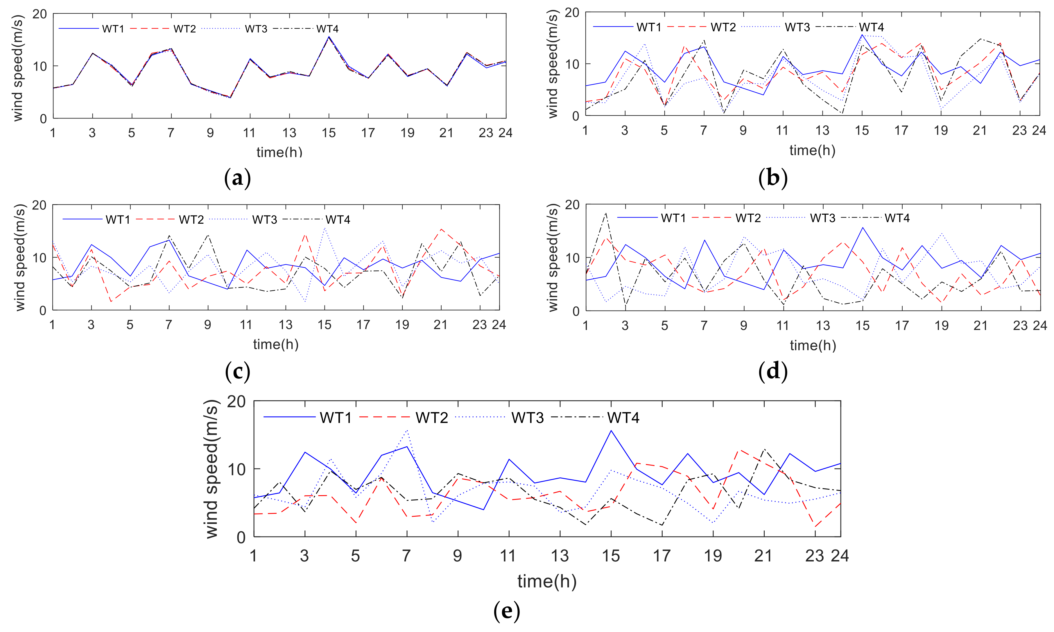
Then the method proposed in Section 2.3 is applied to generate the random numbers of the correlated wind speeds, in order to get the wind speed time series of all wind farms, which are shown in Appendix B, Figure B1, and subsequently transformed them into power production to obtain the random numbers of wind power.
5.3. Optimal Spinning Reserve Capacity with Different Wind Speed Correlation
The installed capacity of the wind generator is 180 MW. The confidence level β is 0.9. The spinning reserve capacities of different wind speed correlations from 15:00 to 24:00 in one day are shown in Table 2.
From Table 2, it can be seen that the up and down spinning reserve capacities rise with the increase of wind speed correlations. Wind speed with positive correlation will strengthen the synchronization (simultaneous increase and decrease) of different wind turbines’ power output and increase the fluctuation of total wind power output. Therefore, compared with no correlation, the power system needs more up and down spinning reserve capacities. However, for the wind farms with negative wind speed correlation, their outputs can be complementary, so that the wind power output of the whole system becomes smooth. Therefore, the up and down spinning reserve capacity is smaller than in the case without considering wind speed correlation. Hence, the wind speed correlation has an important impact on the spinning reserve capacity of the power system with high wind power penetration, so it should not be ignored.
5.4. The Impact of Wind Speed Correlation on Spinning Reserve under Different Wind Power Capacities
Figure 2a–d shows the up and down spinning reserve capacities with different wind speed correlations, in which the wind power installed capacities are 180 and 360 MW, and the confidence level β is 0.9.
Figure 2 illustrates that the wind speed correlation has a greater influence on the spinning reserve capacity with the increase of the wind power installed capacity. In particular, the wind power forecast error will increase with time, and the wind output with positive correlation is more fluctuating; therefore, the difference in the spinning reserve capacity between the positive and the negative correlation becomes greater with time. Meanwhile, the up spinning reserve is more easily affected by the wind speed correlation than the down spinning reserve. Therefore, it is necessary to consider the influence of wind speed correlation on spinning reserve in the power system with the large-scale wind power integration.
5.5. The Effect of Wind Speed Correlation on Expected Energy Not Served
Table 3 lists the influence of the wind speed correlation on EENS, when the confidence level β is 0.9. The wind power installed capacities are 90, 180, 270, and 360 MW, respectively.
As shown in Table 3, with the increase of the wind speed correlation, the EENS increases. When the wind speed correlation goes up, the wind farm output is more volatile, especially in the case of a high positive correlation; in that situation, the prediction deviation of wind power becomes larger, leading to a greater standard deviation of electricity demand in the whole power system, which gives rise to the increase of EENS. Meanwhile, EENS goes up as the wind power capacity rises.
5.6. Optimization Results under Different Confidence Levels
As shown above in Table 4, where the wind power installed capacity is 180 MW and the wind speed correlation is moderate, with an increasing confidence level the EENS decreases; however, the spinning reserve capacity and the total cost rise. Therefore, it is important to choose an appropriate confidence level to provide the trade-off between security and economy.
6. Conclusions
This paper proposes an optimal model of spinning reserve capacity with wind speed correlation, in which the load forecast error, wind power output prediction error, and unit forced outage rate of the uncertainty factors are considered. At the same time, the model is solved by the QPSO algorithm based on stochastic simulation. The main conclusions of this paper are as follows:
- With an increase of wind speed correlation, the fluctuation of the wind farm output is greater, so the spinning reserve capacity should be increased. However, when the wind speed correlation is negative, the outputs of wind farms can be complementary, so the spinning reserve capacity should be reduced in comparison to non-correlation;
- With the increase of wind power installed capacity, the wind speed correlation has a greater effect on the spinning reserve capacity;
- The relationship between the total cost and confidence level of the test system was analyzed so that the results can provide decision support for dispatchers in the balance between reliability and economy.
Author Contributions
This paper is a collaborative effort among the authors. J.Z. conceived the main ideas presented in the paper and conducted the main analysis; H.Z. performed simulations and wrote part of the first draft. L.Z. and J.G. provided an in-depth review and revised the final version thoroughly together.
Funding
This research was funded by Department of Science and Technology of Sichuan Province, China (2017GZ0263) and Department of Science and Technology of Cheng Du Province, China (2016-HM01-00275-SF).
Conflicts of Interest
The authors declare no conflict of interest.
Appendix A

Table A1.
Forecast load.
| Time/h | Load/MW | Time/h | Load/MW | Time/h | Load/MW | Time/h | Load/MW | Time/h | Load/MW | Time/h | Load/MW |
|---|---|---|---|---|---|---|---|---|---|---|---|
| 1 | 960 | 5 | 840 | 9 | 1305 | 13 | 1485 | 17 | 1440 | 21 | 1380 |
| 2 | 900 | 6 | 870 | 10 | 1425 | 14 | 1500 | 18 | 1440 | 22 | 1395 |
| 3 | 870 | 7 | 960 | 11 | 1485 | 15 | 1500 | 19 | 1395 | 23 | 1305 |
| 4 | 840 | 8 | 1140 | 12 | 1500 | 16 | 1455 | 20 | 1380 | 24 | 1080 |
Table A2.
Data of thermal power generators.
| 1–5 | 20 | 80 | 0.009 8 | 7.884 | 531.3 | 100 | 5 | 5 | 20 | 20 | 1.81 | 0.27 | 0.02 |
| 6–10 | 55 | 100 | 0.012 9 | 6.373 | 514.5 | 120 | 3 | 3 | 30 | 30 | 1.33 | 0.20 | 0.04 |
| 11–15 | 75 | 150 | 0.002 3 | 9.616 | 353.1 | 50 | 2 | 2 | 70 | 70 | 1.27 | 0.19 | 0.04 |
| 16 | 160 | 350 | 0.002 4 | 9.385 | 368.4 | 80 | 2 | 2 | 40 | 40 | 1.57 | 0.22 | 0.08 |
Appendix B
Figure B1.
Wind speed time series with different correlation coefficients: (a) high correlation, (b) moderate correlation, (c) low correlation, (d) negative correlation, and (e) no correlation.
Figure B1.
Wind speed time series with different correlation coefficients: (a) high correlation, (b) moderate correlation, (c) low correlation, (d) negative correlation, and (e) no correlation.
References
- Lin, Z.; Luo, L. Analysis of wind power output characteristics in Fujian and its impact on power grid. Electr. Power Construct. 2011, 32, 18–23. (In Chinese) [Google Scholar]
- Zhang, G.; Wang, X. Study on benefits and costs of spinning reserve capacity in power market. Autom. Electr. Power Syst. 2000, 24, 14–18. (In Chinese) [Google Scholar]
- Zhang, G.; Wu, W.; Zhang, B. Optimization of operation reserve coordination considering wind power integration. Autom. Electr. Power Syst. 2011, 12, 4–9. (In Chinese) [Google Scholar]
- He, J.; Sun, H.; Liu, M. Extended state-space partitioning based operating reserve risk assessment for power grid connected with wind farms. Power Syst. Technol. 2012, 3, 43–48. (In Chinese) [Google Scholar]
- Bo, Y.; Ming, Z.; Gengyin, L. A coordinated dispatching model considering generation and operation reserve for wind power integrated power system based on ELNSR. Power Syst. Technol. 2013, 37, 800–807. (In Chinese) [Google Scholar]
- Sahin, C.; Shahidehpour, M.; Erkmen, I. Allocation of hourly reserve versus demand response for security-constrained scheduling of stochastic wind energy. IEEE Trans. Sustain. Energy 2013, 4, 219–228. [Google Scholar] [CrossRef]
- Chen, H.; Kong, Y.; Li, G.; Bai, L. Conditional value-at-risk-based optimal spinning reserve for wind integrated power system. Int. Trans. Electr. Energy Syst. 2016, 26, 1799–1809. [Google Scholar] [CrossRef]
- Reddy, S.S.; Bijwe, P.R. Joint energy and spinning reserve market clearing incorporating wind power and load forecast uncertainties. IEEE Syst. J. 2015, 9, 152–164. [Google Scholar] [CrossRef]
- Zugno, M.; Conejo, A.J. A robust optimization approach to energy and reserve dispatch in electricity markets. Eur. J. Oper. Res. 2015, 247, 659–671. [Google Scholar] [CrossRef] [Green Version]
- Cobos, N.G.; Arroyo, J.M.; Street, A. Least-cost reserve offer deliverability in day-ahead generation scheduling under wind uncertainty and generation and network outages. IEEE Trans. Smart Grid 2016. [Google Scholar] [CrossRef]
- Li, C.; Yun, J.; Tao, D.; Liu, F.; Ju, Y.; Yuan, S. Robust Co-optimization to energy and reserve joint dispatch considering wind power generation and zonal reserve constraints in real-time electricity markets. Appl. Sci. 2017, 7, 680. [Google Scholar] [CrossRef]
- Li, Y.; Li, W.; Yu, J.; Zhao, X. Probabilistic optimal power flow considering correlations of wind speeds following different distributions. IEEE Trans. Power Syst. 2014, 29, 1847–1854. [Google Scholar] [CrossRef]
- Chen, F.; Li, F.; Wei, Z.; Sun, G.; Li, J. Reliability models of wind farms considering wind speed correlation and WTG outage. Electr. Power Syst. Res. 2015, 119, 385–392. [Google Scholar] [CrossRef]
- Xie, M.; Xiong, J. Two-stage compensation algorithm for dynamic economic dispatching considering copula correlation of multi-wind farms generation. IEEE Trans. Sustain. Energy 2017, 8, 763–771. [Google Scholar] [CrossRef]
- Liu, P.L.; Der Kiureghian, A. Multivariate distribution models with prescribed marginals and co-variances. Probab. Eng. Mech. 1986, 1, 105–112. [Google Scholar] [CrossRef]
- Dagang, L.; Yu, X.; Wang, G. Global probabilistic seismic capacity analysis based on an improved point estimation method. World Earthq. Eng. 2008, 4, 7–14. [Google Scholar]
- Wang, Y.; Xu, C.; Yue, W. A stochastic programming model for spinning reserve of power grid containing wind farms under constraint of time-varying reliability. Power Syst. Technol. 2013, 5, 1311–1316. [Google Scholar]
- Sun, J.; Fang, W.; Wu, X.; Palade, V.; Xu, W. Quantum-behaved particle swarm optimization: analysis of individual particle behavior and parameter selection. Power Syst. Technol. 2013, 5, 1311–1316. [Google Scholar] [CrossRef] [PubMed]
Figure 1.
Flow chart of the quantum-behaved particle swarm optimization (QPSO) algorithm.

Figure 2.
Spinning reserve comparisons under wind speed correlation: (a) up spinning reserve capacity with wind speed correlation under a wind power installed capacity of 180 MW; (b) down spinning reserve capacity with wind speed correlation under a wind power installed capacity of 180 MW; (c) up spinning reserve capacity with wind speed correlation under a wind power installed capacity of 360 MW; (d) down spinning reserve capacity with wind speed correlation under wind power installed capacity of 360 MW.
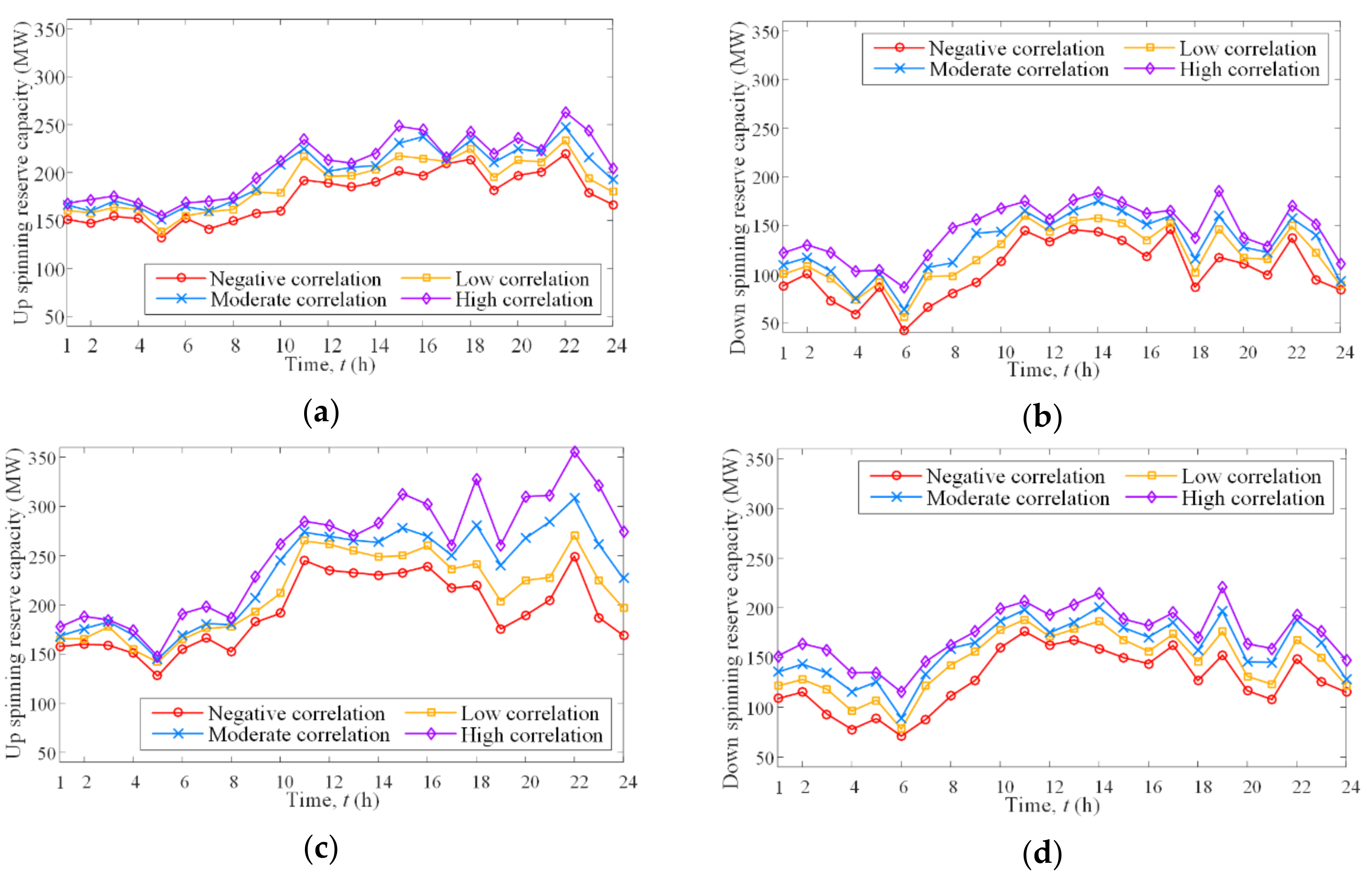
Table 1.
The correlation coefficients of wind speed.
| Correlation Coefficient ρ | Correlation Coefficient ρ0 |
|---|---|
| 0.9 | 0.9230 |
| 0.5 | 0.5125 |
| 0.1 | 0.1022 |
| −0.5 | −0.5118 |
Table 2.
Results of the spinning reserve under different wind speed correlations.
| Type | Spinning Reserve (MW) | Time/h | |||||||||
|---|---|---|---|---|---|---|---|---|---|---|---|
| 15 | 16 | 17 | 18 | 19 | 20 | 21 | 22 | 23 | 24 | ||
| High correlation | Up | 248.5 | 244.5 | 216.1 | 242.7 | 219.5 | 235.9 | 223.6 | 263.2 | 243.3 | 204.5 |
| Down | 173.8 | 162.2 | 165.6 | 137.6 | 185.8 | 137.6 | 128.7 | 170.6 | 151.6 | 111 | |
| Moderate correlation | Up | 230.7 | 237.6 | 214.7 | 233.4 | 210.6 | 224.4 | 222.4 | 247.1 | 215.4 | 192.5 |
| Down | 164.9 | 150.7 | 159.9 | 116.2 | 159.4 | 127.7 | 122.3 | 157.5 | 140.1 | 92.2 | |
| Low correlation | Up | 217.5 | 214.7 | 211.7 | 224.7 | 194.9 | 212.9 | 211.3 | 233.5 | 193.8 | 179.9 |
| Down | 152.9 | 134.8 | 152.7 | 101.9 | 146.3 | 116.7 | 115.1 | 149.2 | 121.9 | 88.7 | |
| No correlation | Up | 212.7 | 206.7 | 210.9 | 220.9 | 190.4 | 208.9 | 210.5 | 228.8 | 188.6 | 172.1 |
| Down | 146.2 | 129.7 | 149.9 | 97.5 | 138.8 | 112.2 | 109.5 | 142.8 | 107.5 | 85.1 | |
| Negative Correlation | Up | 201.3 | 196.6 | 209.3 | 213.9 | 181.8 | 197.2 | 201.3 | 219.2 | 178.8 | 166.7 |
| Down | 134.6 | 118.1 | 145.8 | 86.5 | 117.2 | 110.9 | 98.8 | 137 | 94.2 | 83.88 | |
Table 3.
Effect of wind speed correlation on expected energy not served (EENS).
| Wind Power Installed Capacity/MW | EENS/MW·h | |||
|---|---|---|---|---|
| High Correlation | Moderate Correlation | Low Correlation | Negative Correlation | |
| 90 | 3.74 | 2.91 | 1.44 | 1.03 |
| 180 | 5.63 | 3.48 | 2.16 | 1.45 |
| 270 | 9.51 | 5.49 | 4.52 | 2.17 |
| 360 | 15.36 | 9.64 | 6.20 | 4.36 |
Table 4.
Optimal dispatch results with different confidence levels.
| Confidence level | 0.80 | 0.85 | 0.90 | 0.95 |
| Total cost/USD | 424,259 | 426,506 | 427,838.8 | 430,447.4 |
| Generation cost/USD | 409,212.3 | 414,038.8 | 416,662.4 | 420,138.6 |
| Reserve cost/USD | 6326.7 | 6857.2 | 7696.4 | 9159.6 |
| EENS/MW·h | 8.72 | 5.61 | 3.48 | 1.47 |
| Up spinning reserve capacity/MW | 3756.9 | 4145.3 | 4793.0 | 5712.6 |
| Down spinning reserve capacity /MW | 2917.6 | 3286.2 | 3450.6 | 3742.3 |
© 2018 by the authors. Licensee MDPI, Basel, Switzerland. This article is an open access article distributed under the terms and conditions of the Creative Commons Attribution (CC BY) license (http://creativecommons.org/licenses/by/4.0/).
Share and Cite
MDPI and ACS Style
Zhang, J.; Zhuang, H.; Zhang, L.; Gao, J. Spinning Reserve Capacity Optimization of a Power System When Considering Wind Speed Correlation. Appl. Syst. Innov. 2018, 1, 21. https://doi.org/10.3390/asi1030021
AMA Style
Zhang J, Zhuang H, Zhang L, Gao J. Spinning Reserve Capacity Optimization of a Power System When Considering Wind Speed Correlation. Applied System Innovation. 2018; 1(3):21. https://doi.org/10.3390/asi1030021
Chicago/Turabian StyleZhang, Jianglin, Huimin Zhuang, Li Zhang, and Jinyu Gao. 2018. "Spinning Reserve Capacity Optimization of a Power System When Considering Wind Speed Correlation" Applied System Innovation 1, no. 3: 21. https://doi.org/10.3390/asi1030021