Article

Modeling the Monthly Distribution of MODIS Active Fire Detections from a Satellite-Derived Fuel Dryness Index by Vegetation Type and Ecoregion in Mexico

by
Daniel José Vega-Nieva
1,
María Guadalupe Nava-Miranda
2,
Jaime Briseño-Reyes
1,*,
Pablito Marcelo López-Serrano
2,
José Javier Corral-Rivas
1,
María Isabel Cruz-López
3,
Martin Cuahutle
3,
Rainer Ressl
3,
Ernesto Alvarado-Celestino
4 and
Robert E. Burgan
5,†
1
Facultad de Ciencias Forestales, Universidad Juárez del Estado de Durango, Río Papaloapan y Blvd., Durango S/N Col. Valle del Sur, Durango 34120, Mexico
2
Instituto de Silvicultura e Industria de la Madera, Universidad Juárez del Estado de Durango, Boulevard del Guadiana 501, Ciudad Universitaria, Torre de Investigación, Durango 34120, Mexico
3
Comisión Nacional para el Conocimiento y Uso de la Biodiversidad (CONABIO), Liga Periférico-Insurgentes Sur 4903, Parques del Pedregal, Del. Tlalpan, Mexico City 14010, Mexico
4
School of Environmental and Forest Sciences, Mailbox 352100, University of Washington, Seattle, WA 98195, USA
5
Rocky Mountain Research Station, USDA Forest Service, 1505 Khanabad Drive, Missoula, MT 59802, USA
*
Author to whom correspondence should be addressed.
Retired.
Submission received: 24 November 2023 / Revised: 18 December 2023 / Accepted: 22 December 2023 / Published: 26 December 2023
(This article belongs to the Special Issue Remote Sensing of Wildfire: Regime Change and Disaster Response)

Abstract

:
The knowledge of the effects of fuel dryness on fire occurrence is critical for sound forest fire management planning, particularly in a changing climate. This study aimed to analyze the monthly distributions of MODIS active fire (AF) detections and their relationships with a fuel dryness index (FDI) based on satellite-derived weather and vegetation greenness. Monthly AF distributions showed unimodal distributions against FDI, which were described using generalized Weibull equations, fitting a total of 19 vegetation types and ecoregions analyzed in Mexico. Monthly peaks of fire activity occurred at lower FDI values (wetter fuels) in more hygrophytic ecosystems and ecoregions, such as wet tropical forests, compared to higher fire activity in higher FDI values (drier fuels) for the more arid ecosystems, such as desert shrublands. In addition, the range of fuel dryness at which most monthly fire activity occurred was wider for wetter vegetation types and regions compared to a narrower range of fuel dryness for higher monthly fire occurrence in the more arid vegetation types and ecoregions. The results from the current study contribute towards improving our understanding of the relationships between fuel dryness and fire occurrence in a variety of vegetation types and regions in Mexico.

1. Introduction

Understanding the patterns of fire occurrence and its response to climate is vital to fire risk mitigation and fuel management [1]. Prediction of forest fire ignition patterns may aid in forest fire-prone areas surveillance and monitoring, in prioritizing forest fuel treatments, and in fire suppression resources allocation planning [2,3,4,5]. Awareness of fire occurrence can help mitigate the environmental and economic impact of fire events [6] by improving decision making in strategic fire management planning (e.g., [7,8,9]). Under scenarios of climate change and concomitant projected changes in fire regimes (e.g., [10,11,12]), it is vital to count on reliable tools for monitoring the impact of changing weather on fuel dryness conditions and expected fire occurrence patterns.
Fuel moisture proxies have been found to have a strong influence on fire activity (e.g., [13,14,15]). Consequently, several studies relating fire occurrence to climatic spatial data (e.g., [16,17,18]) have provided useful information to orient long-term planning of fire management as affected by climatic variables. Other studies have utilized weather variables (e.g., [19,20,21]) or weather-based fire danger indices (e.g., [22,23,24]) to explain fire occurrence under changing weather conditions.
In addition, because of the ability of satellite data to map live fuel moisture at finer spatial scales (e.g., [25,26,27]), some studies have also utilized satellite measurements of fuel greenness to analyze fire occurrence (e.g., [28,29,30]) or its influence on burn probability (e.g., [31]). Furthermore, some studies have successfully combined both weather-based dead fuel moisture estimates and satellite observations of live fuel greenness to characterize fire occurrence risk (e.g., [32,33,34]). Several of these previous studies (e.g., [35,36,37]) have highlighted the need to understand how the influence of fuel dryness on fire activity varies under contrasting bioclimatic regions and fuel types. Nonetheless, further research is required on the relationships of weather and satellite-based estimates of fuel moisture and fire occurrence for a variety of vegetation types and climatic regions.
Due to its extension and its recognized vegetation megadiversity [38,39], Mexico provides an interesting opportunity for exploring the conjectural relationship between fire occurrence and fuel dryness for a large variety of vegetation types and climatic conditions, ranging from arid shrubland ecosystems to tropical rain forests (e.g., [40,41,42]). Previous studies in Mexico, mainly at local to regional scales, have evaluated the role of weather variables such as precipitation (e.g., [43,44,45]), temperature (e.g., [46,47,48]), relative moisture [49], or satellite-based fuel greenness (e.g., [50,51]) on fire occurrence risk. In contrast, at a national scale, studies relating to fire occurrence and fuel dryness are still very scarce (e.g., [52,53,54]). These previous studies have highlighted the need to further understand the variations in the relationships of fuel dryness and fire by region in the country (e.g., [52,54]).
The previous study by Vega-Nieva et al. [40] developed a fuel dryness index (FDI) for the Mexican vegetation types based on the fire potential index (FPI) of Burgan et al. [32]. The FPI, which combines weather and satellite information, has been largely utilized in the USA (e.g., [6,34,55]) and Europe [35,36,37,56,57] for fire danger prediction and mapping. The development of its adaptation for Mexico involved considering observed minimum and maximum dead fuel moisture and NDVI values for the study area, as detailed by [40]. Based on this fuel dryness index, the previous study of [40] further developed temporal models to predict the number of MODIS active fire detections for the main vegetation types and climatic regions of Mexico. Whereas these temporal models are useful for predicting the expected number of active fires at a given date for each vegetation type in Mexico, they offer no information on the distribution of those active fires within these vegetation types. Furthermore, they do not reveal how these distributions within vegetation types might vary between dates with different fuel dryness conditions. In addition, there is no previous national-scale study in Mexico that has attempted to analyze the temporal variations in the distribution of active fires within vegetation types in relation to a satellite-derived fuel dryness index.
The current study aimed to model the monthly distribution of MODIS active fire detections from a fuel dryness index for the main vegetation types and regions in Mexico. The specific goals were:
(1) To test simple distribution models for predicting the monthly distribution of active fires (AF) from the fuel dryness index FDI for a total of 19 types of vegetation by regions of the country in the period 2011–2015;
(2) To explore models with expanded coefficients to explain the variation in the shapes of AF distributions by the FDI between months and years of varying fuel dryness conditions for the vegetation types and regions analyzed.

2. Materials and Methods
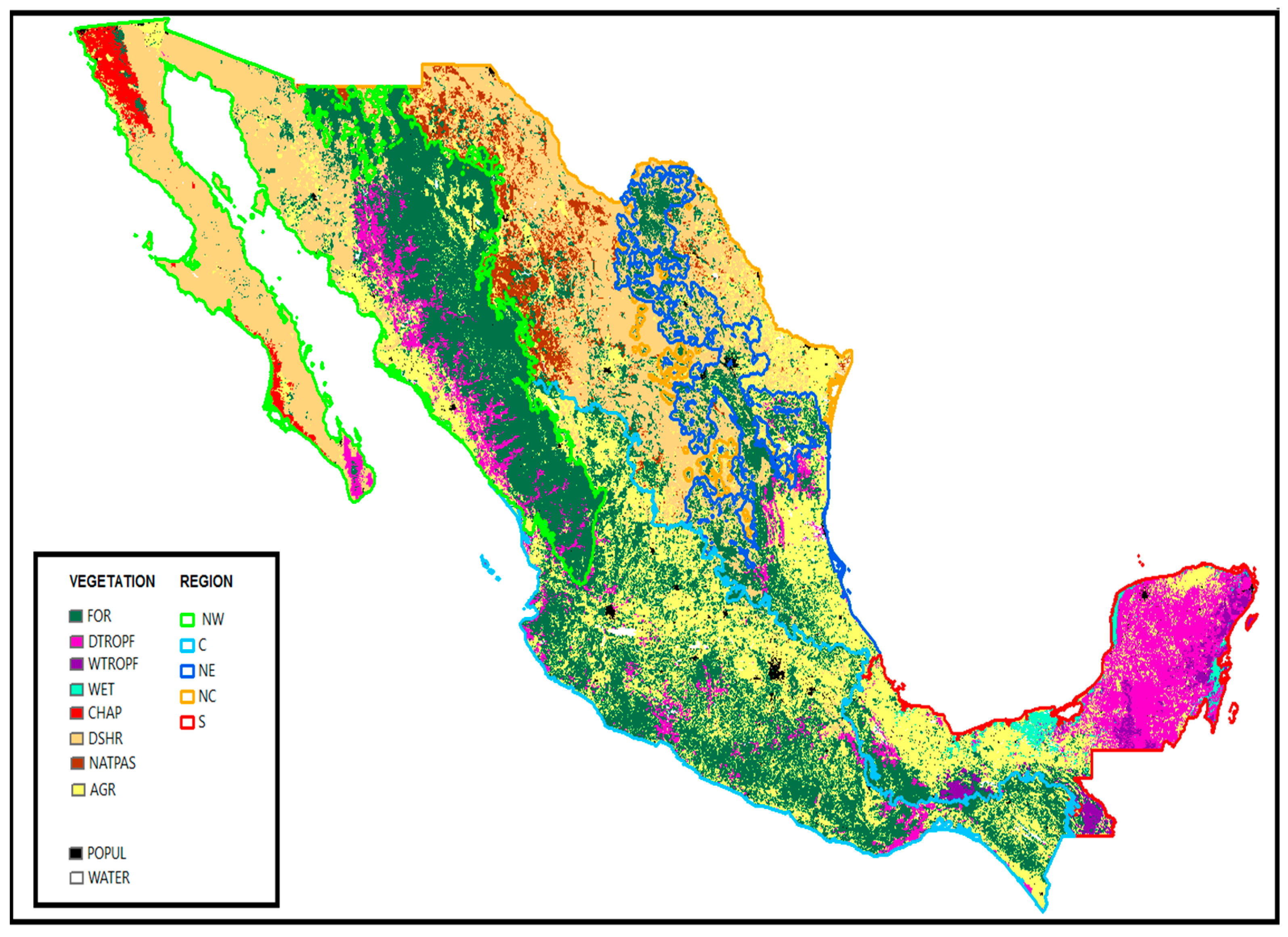
2.1. Study Area

The study area was Mexico. Vegetation types (Figure 1) were defined following Vega-Nieva et al.’s [40] reclassification of the National Institute of Geography and Statistics (INEGI in Spanish) land use and vegetation map (INEGI Land Use Map Series V, 1:25,000 URL: http://www.inegi.org.mx/geo/contenidos/recnat/usosuelo/, accessed on 20 December 2023). Accordingly, five study regions were defined based on the North American level 3 ecoregions map (URL: https://www.epa.gov/eco-research/ecoregions-north-america, accessed on 20 December 2023), taking into account the patterns of fire occurrence observed in previous studies [40,54]. This resulted in a total of 19 vegetation and region units to be analyzed (Figure 1).

2.2. Fuel Dryness Index Inputs

Fuel dryness index inputs were daily images of moisture content of dead fuels of 100 h (H100) [58,59,60] and 10-day MODIS NDVI composites at 1 km of spatial resolution, calculated by the National Commission for Knowledge and Use of Biodiversity (CONABIO) following the methodology described by [40,60]. The period of study was 2011 to 2015, defined by H100 availability from CONABIO at the time of the study. The inputs for H100 images included daily temperature and relative humidity from MODIS atmospheric profiles, together with precipitation from the TRMM satellite, as described in [60].

2.3. Fuel Dryness Index (FDI) Calculation

The fuel dryness index (FDI) [40] represents an integrated estimate of dead and live fuel moisture, following the structure of the FPI [32]. The index considers relative dead and live fuel moisture, scaled with reference to its historical minimum and maximum values [40]. High FDI values represent dry fuels, reaching FDI values of up to 100, its maximum historical fuel dryness level (i.e., minimum observed coarse dead fuel moisture and live vegetation greenness for every pixel), while low FDI values (e.g., <30–40) represent wet fuels with high live fuel greenness and high dead moisture conditions [32,40].
The FDI was calculated following the adaptation proposed by [40] for the Mexican vegetation types of the FPI [32], based on Equations (1) to (5):
FDI = (1 − LR)·(1 − MR)·100
where
LR: live fuel ratio from 10-day composite NDVI images, following Equations (2) to (4).
MR: 100 h dead fuels moisture ratio, following Equation (5).
The calculation of the first component of the index, live ratio (LR), was performed utilizing Equations (2) to (4), following [32,40]:
LR = RG·LRmax/100
where RG is relative greenness, following Equation (3):
RG = (NDVI0NDVImin)/(NDVImaxNDVImin)·100
where NDVI0 is the 10 days observed NDVI for every pixel, and NDVImin and NDVImax are the historical minimum and maximum NDVI values calculated for every pixel, respectively.
LRmax is the maximum observed live ratio value for each pixel.
LRmax was calculated based on observed maximum NDVI values in Mexico following Equation (4) [40]:
LRmax = 30 + 30·(NDVImax − 125)/(255 − 125)
where NDVImax = maximum NDVI calculated for every pixel. The values 125 and are the absolute minimum and maximum of the maximum NDVI values observed for Mexico [40].
The second component of the index, 100 h dead fuels moisture ratio (MR), was calculated following Equation (5) [40]:
MR = (H100 − Hmin)/(HmaxHmin)
where H100 is the 100 h dead fuel moisture estimated value, and Hmax and Hmin are the maximum and minimum H100 values for every pixel, respectively.

2.4. Observed Monthly Number and Percentage of Active Fires by FDI Values

MODIS active fires were downloaded in point shapefile format for the study period from the Forest Fire Early Warning System of the National Commission for Knowledge and Use of Biodiversity (CONABIO) (URL: http://incendios.conabio.gob.mx/, accessed on 20 December 2023) [60]. Active fire data from CONABIO were calculated based on the MODIS fire detection algorithm by Giglio et al. [61], together with the false alarm filtering process described by Cruz-López et al. [62]. This false alarm filtering involves considering local thresholds for brightness temperature [62] to prevent active fire commission errors caused by very high albedo or sunlight. In addition, various masks are also considered, including a NDVI and vegetation mask to discard desert areas without vegetation together with a mask of stable lights, the latter generated by the U.S. Air Force Defense Meteorological Satellite Program (DMSP) Operational Linescan System (OLS) satellite images (URL: https://www.ncei.noaa.gov/products/dmsp-operational-linescan-system, accessed on 20 December 2023), as described in [62].
We extracted the FDI value for each active fire on the corresponding day. The percentage of active fires observed for each i value of the FDI for each j month-year was calculated for every vegetation type and region following Equation (6):
% AFij = Nij/NTj·100
where % AFij = observed percentage of active fires for each i value of FDI for each j month-year, Nij: observed number of active fires for each i value of FDI for each j month-year, and NTj: total number of observed active fires for each j month-year.
Based on % AFij values, the accumulated values of the percentage of active fires (Ac.% AFij) were calculated for each i value of the FDI for each j month-year for every vegetation type-region. Monthly % AFij and Ac.% AFij values were calculated for the main months of the fire season in the study area (from January to May [40]) for the years of study.

2.5. Modeling the Accumulated % AF from FDI Values

Two approaches were tested for modeling the observed monthly distributions of Ac.% AFij by FDI values. In the first approach, the observed accumulated percentage of active fires was modeled for every vegetation type with a single Weibull equation following Equation (7):
Ac.% AFij = 1 − exp(−((FDIij/b)c))
where Ac.% AFij: observed monthly accumulated percentage of active fires for each i value of FDI for each j month-year; FDIij: i observed fuel dryness index value for each j month-year; and b and c are coefficients.
In the second approach, it was hypothesized that b and c coefficients from Equation (7) would vary each month and year related to fuel dryness conditions, as reflected by the average monthly FDI value observed for every vegetation type. In this approach, Equation (7) was expanded to a generalized family of Weibull curves by expanding the b and c coefficients from Equation (7) for each vegetation type and region. We tested lineal (Equations (8) and (9)) or power expressions ((10) and (11)). For the lineal formulation, b and c coefficients from Equation (7) were expanded as:
b = b1 + b2·FDImean
c = c1 + c2·FDImean
where b and c are the general Weibull model coefficients in Equation (7), b1, b2, c1, and c2 are model coefficients, and FDImean: is the average FDI value for each vegetation type each month.
For the power formulation:
b = b1·FDImean b2
c = c1·FDImean c2
where b and c are the general Weibull model coefficients in Equation (7), b1, b2, c1, and c2 are model coefficients, and FDImean: is the average FDI value for each vegetation type each month.
The candidate models were evaluated using the coefficient of determination for nonlinear regression (R2), together with root-mean-square error (RMSE) and model Bias as statistical criteria [63].

3. Results

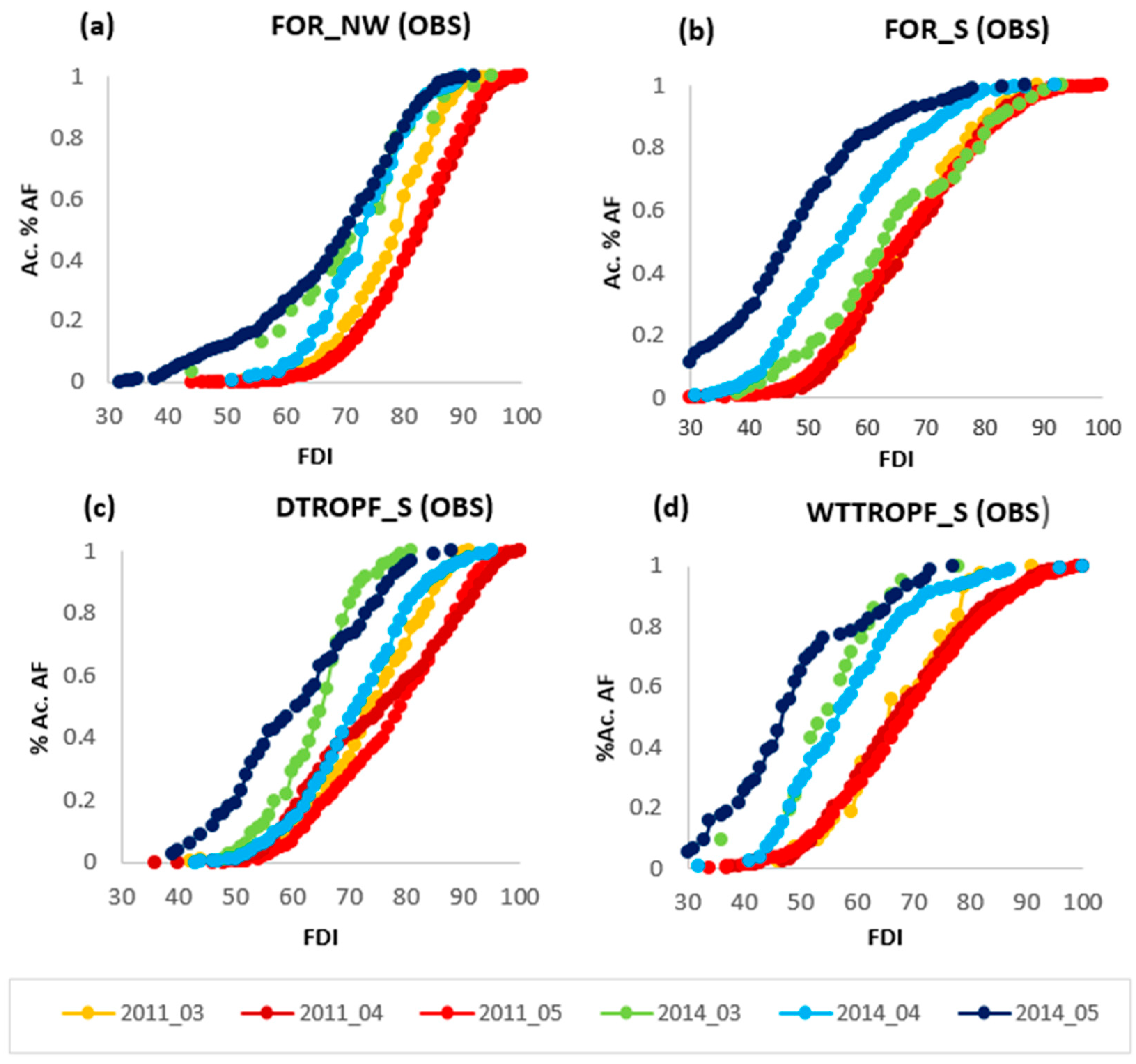
3.1. Observed % AF Distributions by FDI Value

The observed distributions of the accumulated percentage of active fires using the FDI value varied by vegetation type, month, and year. Some illustrative examples for selected vegetation types and regions for months 03–05 of years 2011 (example of dry year) and 2014 (example of wet year) are shown in Figure 2. Differences in the observed Ac.% AF distributions were visible between regions, with the driest regions, such as the temperate forest of the NW region (Figure 2a), which receives comparatively less precipitation (e.g., [40,54]), showing a family of curves with higher observed accumulated percentage of active fires on the higher (drier) FDI values. In contrast, a higher percentage of active fires was observed in lower (wetter) FDI values for the more humid regions and vegetation types, such as temperate or tropical forests from the more humid South region (Figure 2c,d).
For most vegetation types, contrasting differences were observed in the accumulated % AF distributions between dry and wet years. For the dry year 2011 (lines in red and orange), a higher percentage of active fires occurred in the higher (drier) FDI values, compared to a higher percentage of active fires observed in the lower (wetter) FDI values for the more humid year 2014 (curves in blue and green), as shown in Figure 2.
Differences in the shape of the observed Ac.% AF distributions occurred also between months (Figure 2): for most vegetation types, the month 04 (April) showed the highest observed percentage of AF of the year occurring in the driest (highest) FDI values, compared to generally wetter months 03 and 05 (March and May). This trend varied between vegetation types and years (Figure 2), which might be due to differences in the dryness conditions of each particular month between different years and vegetation types.

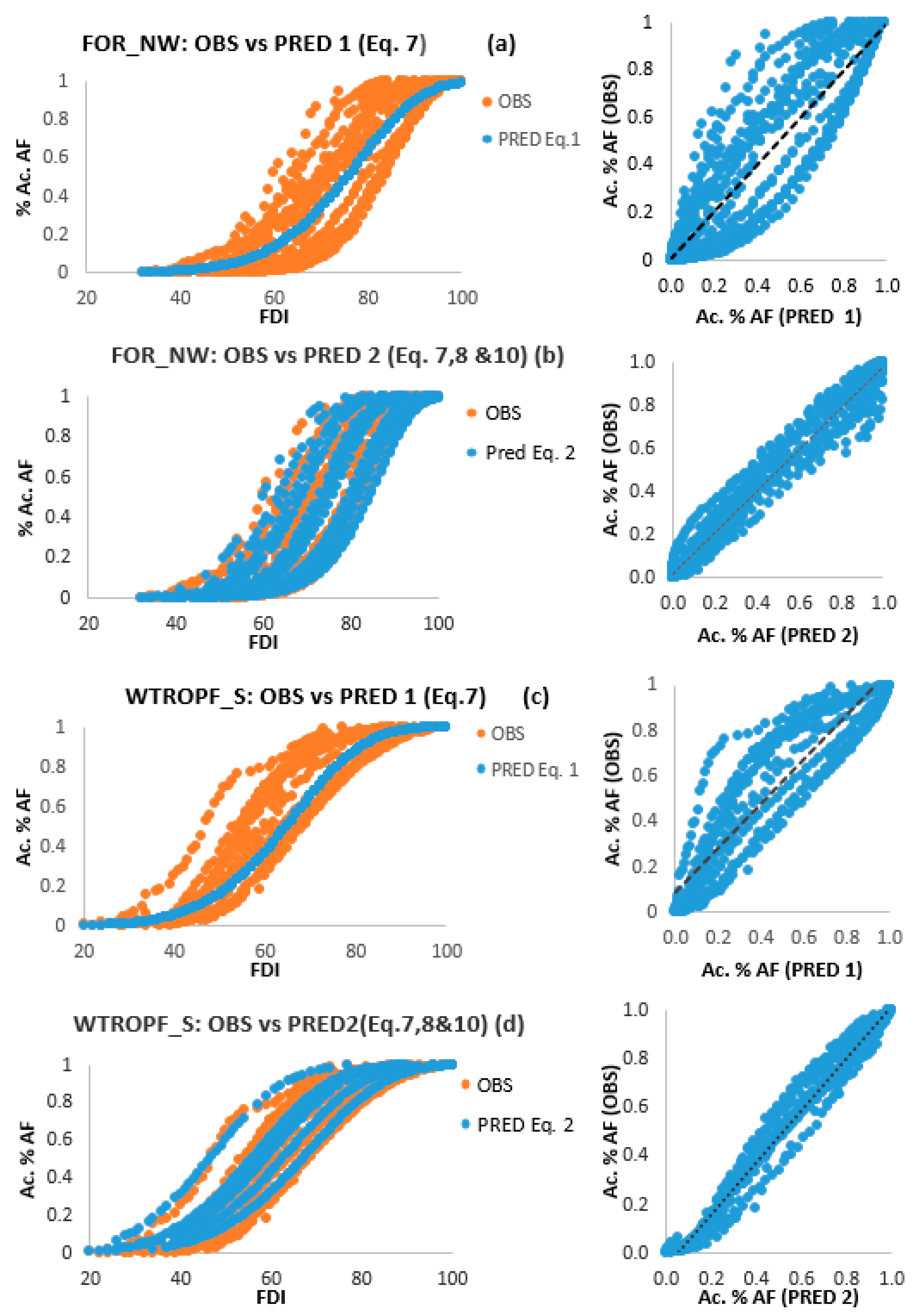
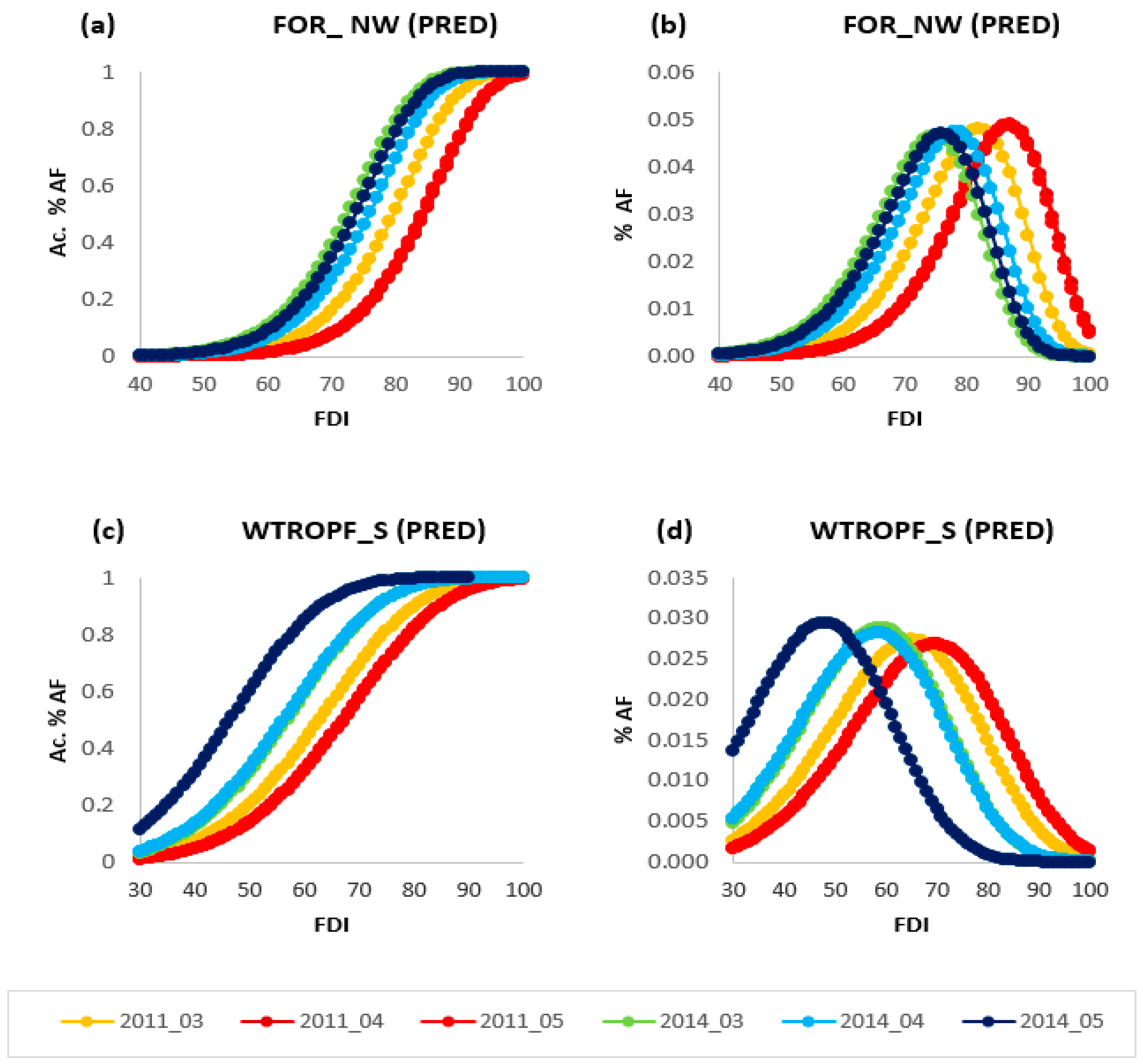
3.2. Predicted % AF Distributions

The best model fits were obtained for all vegetation types with approach 2, utilizing a linear expression for expanding factor b (Equation (8)) and a power model for expanding coefficient c (Equation (11)). The best fit coefficients and goodness of fit values using these expressions are shown in Table 1. The R2 values using the best fit models were higher than 0.95 for 13 and RMSE values lower than 0.1 for 12 of the 19 modeled vegetation types (Table 1). The fits with lower R2 (0.74–0.88) and higher RMSE values (0.11–0.17) were found for temperate forests of the NC region, tropical forests of the NE, wetlands, and shrubby vegetation, although they were better than with approach 1 in all cases.
The first modeling approach—e.g., utilizing a single Weibull equation for each vegetation and region for explaining all the monthly observed % AF distributions—provided lower R2 and RMSE values two to three times higher compared to the second modeling approach—expanding the Weibull coefficients as functions of the observed monthly mean FDI value for each vegetation type.
An example of the comparison of these two modeling approaches can be seen in Figure 3 for two contrasting vegetation types, temperate forest of the NW (Figure 3a,b) and wet tropical forest of the S (Figure 3c,d). It can be seen that whereas modeling strategy 1 with a single Weibull distribution by vegetation type provides an acceptable fit to the average tendency of the observed AF distributions (Figure 3a,c), modeling strategy 2, expanding the Weibull coefficients into a family of Weibull distributions (Figure 3b,d), shows more potential for capturing the monthly variations in the shapes and inflection points of the observed monthly AF distributions.
The b parameter, obtained from Equation (8) from b1 and b2 coefficients (Table 1), corresponds to the value of the FDI where the inflection points of the accumulated % AF distribution occur. In the corresponding de-accumulated % AF distribution, this inflection point defined by the b value represents the value of the FDI where the maximum percentage of active fires occurs. This is illustrated in Figure 4, which shows the predicted accumulated % AF distribution (Figure 4a,c) and the corresponding predicted % AF distribution (Figure 4b,d, respectively) for two contrasting vegetation types (temperate forest of the NW and wet tropical forest of the S region) for the main fire season months of two years: the dry year 2011 and the wet year 2014. For the temperate forest of the NW (Figure 4a,b), the predicted inflection points given by the b coefficient (maximum values in Figure 4b) ranged from 82 to 87 for the dry 2011 year, and they ranged from 75 to 78 for the wetter year 2014 (Figure 4b). In the case of the more humid tropical forest of the S (Figure 4c,d), the predicted maximum values of the % AF curves occurred at lower (wetter) FDI values of 68–72 for the dry year 2011 and of 51–61 for the wetter year 2014 (Figure 4d).
The c parameter from Equation (7), as derived from c1 and c2 (Equation (11)), explains the shape of the AF curve, with higher c values corresponding to steeper curves—e.g., more active fires were found to be occurring on a narrower range of fuel dryness FDI values around the maximum value of the % AF curve—and lower c values representing more flat curves—e.g., active fires are occurring on a higher range of fuel dryness values. Thus, the best fit c1 and c2 coefficients (Table 1) may offer information about how narrow the range of FDI values is where fires occur between vegetation types and regions. For example, in the case of the vegetation type temperate forest (FOR), the highest c1 and c2 values were obtained for the drier NC, NW, and C regions (with best fit values of c2 of 1.15 for NC and 1.05 for NW and C), followed by the more humid NE region (with a best fit c2 value of 0.987), and lower values (c2 of 0.83) were obtained for the temperate forest of the south region, which is the area of highest precipitation in the country. The lowest c2 coefficient values were obtained for the tropical forest of the south (c2 of 0.51), and the highest values were obtained for the most arid vegetation type, desert shrubby vegetation (DSHR), with a c2 value of 1.26 (Table 1). These differences in the c1 and c2 coefficients (Equation (11)) between vegetation types and regions resulted in higher predicted c values (Equation (7)) (i.e., steeper curves) for drier vegetation types and regions (e.g., shrubs, agriculture, and temperate forest of the NC, NW, and C regions) and lower predicted c values (i.e., flatter curves) for the more humid vegetation types and regions such as temperate and tropical forest of the south.

4. Discussion

The observed variations in the FDI and AF between regions support the observations from other studies relating the FPI (e.g., [56,57]) or other fire indices (e.g., [64,65,66]) to fire occurrence across ecoregions, where separated relationships were observed for different climatic and vegetation types. The best fit parameters shown in Table 1 seem to have the potential to capture differences in the shape and inflection points of different vegetation types under varying fuel dryness conditions. The goodness of fit of the monthly active fire spatial distributions utilizing the expanded Weibull model was high for most vegetation types. The lowest R2 values were obtained for vegetation types that either cover relatively small areas and/or have a relatively low number of fires. Perhaps expanding the period of observations in future studies might allow us to improve the models presented in this work for these areas with lower fire occurrence.
The variations in the predicted c-shape coefficients seem to suggest a narrower range of FDI values for observed fire occurrence on the driest vegetation types and regions and, conversely, a wider FDI range for fire activity on the more humid vegetation types and regions. Fires in these latter wetter tropical landscapes are largely altered by agricultural burns (e.g., [42,67,68]), resulting in the possibility of ignitions occurring under wetter conditions because of human ignition.
In general, the predicted inflection points at peaks of fire activity determined by the b coefficient were found at higher FDI values for drier vegetation types. Thus, the predicted maximum fire occurrence was observed at values of up to a FDI of 85–90 for the most arid vegetation types, such as desert shrubs, temperate forests, and agriculture of the NC, NW, and C regions. In contrast, lower maximum values of up to 70–75 were found for the more humid vegetation types, such as temperate and tropical forests of the S. These results suggest that in such more humid regions, more fires occur at lower fuel dryness levels. In addition to the above-mentioned hypothesis of a larger fire occurrence under moist conditions in areas with higher human activity [42], the presence of different fuel types, with different responses to fuel moisture, between contrasting ecosystems might also be influential. In particular, this can be related to previously reported higher moisture thresholds for fire occurrence for more hygrophyte fuels (e.g., [32,69]). For example, Burgan et al. [32] considered a higher extinction moisture (10 h dead fuels moisture threshold for fire occurrence) of 25% for more humid fuels such as short-needle conifers or black spruce. Conversely, fuels in more arid climates, such as chaparral, brush, and grass fuels, were assigned an extinction moisture of 15% by [32]. Similarly, the analysis of fire occurrence in an aridity gradient in Spain by [69] also found that higher dryness thresholds for fire occurrence were required in more arid areas and highlighted the need to account for fuel-specific variations in the relationships between fuel dryness and fire occurrence. For the FDI, these results are consistent with previous temporal analysis of fire occurrence by [40], which also found fire occurrence to be sustained at relatively lower FDI values in wetter ecosystems. They also support the previous relationship between active fires and precipitation reported for the period 2000–2007 by [70] and the previous analysis by [45,71] between fire emissions and precipitation (2011–2014) in three ecoregions in Mexico. Furthermore, these results support the findings with a FPI between four ecoregions in Europe by Sebastian-Lopez et al. [56], where the FPI threshold value at which 75% of the fires occurred was higher for the driest bioclimatic region, compared to the lower FPI threshold values for the wettest regions
Within each vegetation type, our study found that the predicted values of the b parameter varied markedly by month and year, reaching values of the FDI lower than 60 in the wettest months and years. This suggests a strong interannual variability in the spatial distribution of fire ignitions. This observed variation in the relationships between fuel dryness and fire occurrence between different dates agrees with the results of other studies where this relationship differed between months (e.g., [64,72,73]) and between years (e.g., [17,74,75]).
The observed humped shape of the AF distributions against the FDI supports previous analysis of the FPI in other locations (e.g., [6,32,76]), where fire occurrence has also been found to peak at certain FPI values and then decrease above this peak value. These observed humped relationships between fire activity and fuel dryness might be related to a combination of fuel and moisture limitations on fire occurrence, supporting the previous hypothesis of fire occurrence constraints (e.g., [71,77,78]). For the lower range of fuel dryness, decreased fire occurrence might be explained by fuel moisture limitations on fire ignition and spread. This might be related to observations from previous studies that have explored proxies of fuel availability against fire activity (e.g., [18,41,42]). In Mexico, refs. [41,42] found limitations to fire activity in denser and possibly wetter forests, which are also expected to be dominated by timber litter fuels, with lower shrub and grass loads. In this sense, the first results from the current exploratory characterization study relating fuel moisture to fire activity, together with the mentioned previous analysis of fuel availability [41], should be expanded in future predictive studies aiming at formally evaluating the separate contributions of fuel loads and fuel moisture on the occurrence and intensity of active fires.
In addition, for the higher fuel dryness values, it is possible that fuel availability, particularly for the most arid ecosystems, where extremely dry conditions might result in reduced fine fuel load and continuity, might be limiting fire occurrence and propagation (e.g., [20]). This could be related to previous observations of lower fire activity after precedent periods of low precipitation in grass- and shrub-dominated ecosystems, which have been attributed to reduced fine fuel load (e.g., [20]). To corroborate this, a formal evaluation of the effect of antecedent periods of precipitation on fine fuel load accumulation and its effect on fire occurrence could be performed in future studies.
The observed variation in the AF distributions against the FDI between the vegetation types and ecoregions analyzed agrees with the contrasting distributions found in the literature for a similar FPI. For example, the observed AF distributions for the temperate forests of the NW region (Figure 4b) have relatively similar behavior to the fire activity distributions by FPI values from the studies of Burgan et al. [32] or Schneider et al. [6] in California, where fire activity peaked at FPI values of approximately 70–80. In contrast, the higher fire activity observed in wet tropical forests of the S region at lower FDI values (Figure 4c,d) is relatively similar to the observations by Yunhao et al. [76] in tropical forests in Malaysia, where more than 90% of the cumulative MODIS active fire percentage was observed at a FPI value of 60.
The generalized expanded Weibull formulation proposed in the current study seems to offer the potential to capture the variation in the relationships between fuel dryness and the distributions of fire occurrence, observed both between months and years of different fuel moisture levels and between different vegetation types and regions and could be tested elsewhere. The current study is the first analysis of monthly active fire distributions against a satellite-retrieved fuel dryness index in Mexico. Although it represents a useful first step in improving our understanding of the influence of fuel dryness on the spatial distributions of fire activity for a variety of vegetation types and regions in the country, it should be expanded in future studies. In particular, future studies could build on this analysis and previous temporal analysis of fire occurrence (e.g., [40]), possibly integrating the role of anthropogenic and fuel variables of fire ignition (e.g., [41,42]) to further develop spatio-temporal forecasts of fire occurrence (e.g., [34,79,80]) from both fuel dryness, human factors (e.g., [81]) and fuel availability.

5. Conclusions

This study analyzed the monthly distributions of MODIS active fire occurrence against a satellite fuel dryness index for a total of 19 vegetation types and regions in Mexico. Active fire monthly distributions showed unimodal (i.e., humped) relationships with fuel dryness, which varied between months, years, and vegetation types. The observed variations in the monthly distribution of active fires could be described using generalized Weibull models fitted for every vegetation type and region. Narrower ranges of fuel dryness for fire occurrence were observed for the drier vegetation types and regions, whereas higher fire occurrence in a wider range of fuel moisture conditions was observed for the wetter vegetation types and regions.
The current study is a first step towards improving our understanding of the relationships between fuel moisture and the patterns of fire occurrence for the main vegetation types and regions in Mexico. Our observed differentiated patterns of fire occurrence between vegetation types and climatic ecoregions might be related to varying fuel and climatic limitations and might very possibly also be influenced by anthropogenic ignitions, a point that deserves further analysis. Future studies will focus on analyzing the spatio-temporal effects of both fuel dryness and human factors in fire activity to enhance our understanding of the complex relationships between fuel, weather, and human drivers of fire occurrence.

Author Contributions

D.J.V.-N., M.G.N.-M. and J.B.-R. performed the statistical analysis; J.B.-R. programmed the code for the daily fuel dryness index automated calculation and for the extraction of FDI values to the daily fire hotspots; R.E.B. provided the fire potential index algorithm, upon which much of this research is based; M.I.C.-L., M.C. and R.R. calculated daily H100 and 10-day NDVI composites from satellite information from CONABIO; D.J.V.-N., writing—original draft preparation; J.J.C.-R., P.M.L.-S. and E.A.-C., writing—review and editing. All authors have read and agreed to the published version of the manuscript.

Funding

This research was funded by CONAFOR/CONACYT Projects “CO2-2014-3-252620” and “CO-2018-2-A3-S-131553” for the development and enhancement of a Forest Fire Danger Prediction System for Mexico, funded by the Sectorial Fund for forest research, development, and technological innovation “Fondo Sectorial Para la Investigación, el Desarrollo y la Innovación Tecnológica Forestal”.

Institutional Review Board Statement

Not applicable.

Informed Consent Statement

Not applicable.

Data Availability Statement

MODIS active fire data for Mexico are available for download from the Forest Fire Early Warning System of the National Commission for Knowledge and Use of Biodiversity (CONABIO) (URL: http://incendios.conabio.gob.mx/, accessed on 20 December 2023). Fuel dryness indexes can be visualized in the Forest Fire Danger Forecast System of Mexico, “Sistema de Predicción de Peligro de Incendios Forestales de México”(URL: http://forestales.ujed.mx/incendios2/, accessed on 20 December 2023) and are available upon request to the authors.

Acknowledgments

The authors would like to thank CONAFOR’s personnel for their feedback on the development of a forest fire danger system for Mexico. We would like to thank CONABIO’s personnel for providing access to MODIS active fire data, 10-day NDVI composites, and daily dead fuel moisture images for Mexico for the period of study.

Conflicts of Interest

The authors declare no conflict of interest. The funders had no role in the design of the study, in the collection, analyses, or interpretation of data, in the writing of the manuscript, or in the decision to publish the results.

References

  1. Liu, Z.; Yang, J.; Chang, Y.; Weisberg, P.J.; He, H.S. Spatial Patterns and Drivers of Fire Occurrence and Its Future Trend under Climate Change in a Boreal Forest of Northeast China. Glob. Chang. Biol. 2012, 18, 2041–2056. [Google Scholar] [CrossRef]
  2. Finney, M.A. The Challenge of Quantitative Risk Analysis for Wildland Fire. For. Ecol. Manag. 2005, 211, 97–108. [Google Scholar] [CrossRef]
  3. Hering, A.S.; Bell, C.L.; Genton, M.G. Modeling Spatiotemporal Wildfire Ignition Point Patterns. Environ. Ecol. Stat. 2009, 16, 225–250. [Google Scholar] [CrossRef]
  4. Yang, J.; He, H.S.; Shifley, S.R.; Gustafson, E.J. Spatial patterns of modern period human-caused fire occurrence in the Missouri Ozark Highlands. For. Sci. 2007, 53, 1–15. [Google Scholar]
  5. Chang, Y.; Zhu, Z.L.; Bu, R.C.; Chen, H.W.; Feng, Y.T.; Li, Y.H.; Hu, Y.M.; Wang, Z.C. Predicting fire occurrence patterns with logistic regression in Heilongjiang Province, China. Landsc. Ecol. 2013, 28, 1989–2004. [Google Scholar] [CrossRef]
  6. Schneider, P.; Roberts, D.A.; Kyriakidis, P.C. A VARI-based relative greenness from MODIS data for computing the fire potential index. Remote Sens. Environ. 2008, 112, 1151–1167. [Google Scholar] [CrossRef]
  7. Preisler, H.K.; Westerling, A.L.; Gebert, K.M.; Munoz-Arriola, F.; Holmes, T.P. Spatially explicit forecasts of large wildland fire probability and suppression costs for California. Int. J. Wildland Fire 2011, 20, 508–517. [Google Scholar] [CrossRef]
  8. Mavsar, R.; González-Cabán, A.; Varela, E. The State of Development of Fire Management Decision Support Systems in America and Europe. For. Policy Econ. 2013, 29, 45–55. [Google Scholar] [CrossRef]
  9. Elia, M.; Giannico, V.; Lafortezza, R.; Sanesi, G. Modeling Fire Ignition Patterns in Mediterranean Urban Interfaces. Stoch. Environ. Res. Risk Assess. 2019, 33, 169–181. [Google Scholar] [CrossRef]
  10. Jolly, W.M.; Cochrane, M.A.; Freeborn, P.H.; Holden, Z.A.; Brown, T.J.; Williamson, G.J.; Bowman, D.M. Climate-Induced Variations in Global Wildfire Danger from 1979 to 2013. Nat. Commun. 2015, 6, 7537. [Google Scholar] [CrossRef]
  11. Podschwit, H.R.; Larkin, N.K.; Steel, E.A.; Cullen, A.; Alvarado, E. Multi-Model Forecasts of Very-Large Fire Occurrences during the End of the 21st Century. Climates 2018, 6, 100. [Google Scholar] [CrossRef]
  12. Dupuy, J.L.; Fargeon, H.; Martin-StPaul, N.; Pimont, F.; Ruffault, J.; Guijarro, M.; Hernando, C.; Madrigal, J.; Fernandes, P. Climate Change Impact on Future Wildfire Danger and Activity in Southern Europe: A Review. Ann. For. Sci. 2020, 77, 35. [Google Scholar] [CrossRef]
  13. Urbieta, I.R.; Zavala, G.; Bedia, J.; Gutiérrez, J.M.; San Miguel-Ayanz, J.; Camia, A.; Keeley, J.E.; Moreno, J.M. Fire activity as a function of fire–weather seasonal severity and antecedent climate across spatial scales in southern Europe and Pacific western USA. Environ. Res. Lett. 2015, 10, 114013. [Google Scholar] [CrossRef]
  14. Keyser, A.; Westerling, A. Climate Drives Inter-Annual Variability in Probability of High-Severity Fire Occurrence in the Western United States. Environ. Res. Lett. 2017, 12, 065003. [Google Scholar] [CrossRef]
  15. Jolly, W.M.; Freeborn, P.H.; Page, W.G.; Butler, B.W. Severe Fire Danger Index: A Forecastable Metric to Inform Firefighter and Community Wildfire Risk Management. Fire 2019, 2, 47. [Google Scholar] [CrossRef]
  16. Oliveira, S.; Pereira, J.M.C.; San Miguel-Ayanz, J.; Lourenço, L. Exploring the Spatial Patterns of Fire Density in Southern Europe Using Geographically Weighted Regression. Appl. Geogr. 2014, 51, 143–157. [Google Scholar] [CrossRef]
  17. Parisien, M.A.; Parks, S.A.; Krawchuk, M.A.; Little, J.M.; Flannigan, M.D.; Gowman, L.M.; Moritz, M.A. An Analysis of Controls on Fire Activity in Boreal Canada: Comparing Models Built with Different Temporal Resolutions. Ecol. Appl. 2014, 24, 1341–1356. [Google Scholar] [CrossRef]
  18. Parks, S.A.; Parisien, M.A.; Miller, C.; Dobrowski, S.Z. Fire Activity and Severity in the Western US Vary Along Proxy Gradients Representing Fuel Amount and Fuel Moisture. PLoS ONE 2014, 9, e99699. [Google Scholar] [CrossRef]
  19. Díaz-Avalos, C.; Peterson, D.L.; Alvarado, E.; Ferguson, S.A.; Besag, J.E. Space–Time Modelling of Lightning-Caused Ignitions in the Blue Mountains, Oregon. Can. J. For. Res. 2001, 31, 1579–1593. [Google Scholar]
  20. Littell, J.S.; McKenzie, D.; Peterson, D.L.; Westerling, A.L. Climate and Wildfire Area Burned in Western U.S. Ecoprovinces, 1916–2003. Ecol. Appl. 2009, 19, 1003–1021. [Google Scholar] [CrossRef]
  21. Cardil, A.; Salis, M.; Spano, D.; Delogu, G.; Molina Terrén, D. Large wildland fires and extreme temperatures in Sardinia (Italy). iForest Biogeosci. For. 2014, 7, 162–169. [Google Scholar] [CrossRef]
  22. Di Giuseppe, F.; Pappenberger, F.; Wetterhall, F.; Krzeminski, B.; Camia, A.; Libertá, G.; San Miguel, J. The Potential Predictability of Fire Danger Provided by Numerical Weather Prediction. J. Appl. Meteorol. Climatol. 2016, 55, 2469–2491. [Google Scholar] [CrossRef]
  23. Jolly, W.M.; Freeborn, P.H. Towards Improving Wildland Firefighter Situational Awareness through Daily Fire Behaviour Risk Assessments in the US Northern Rockies and Northern Great Basin. Int. J. Wildland Fire 2017, 26, 574–586. [Google Scholar] [CrossRef]
  24. Sirca, C.; Salis, M.; Arca, B.; Duce, P.; Spano, D. Assessing the performance of fire danger indexes in a Mediterranean area. iForest Biogeosci. For. 2018, 11, 563–571. [Google Scholar] [CrossRef]
  25. Yebra, M.; Dennison, P.; Chuvieco, E.; Riaño, D.; Zylstra, P.; Hunt, R.; Danson, F.M.; Qi, Y.; Jurdao, S. A global review of remote sensing of live fuel moisture content for fire danger assessment: Moving towards operational products. Remote Sens. Environ. 2013, 136, 455–468. [Google Scholar] [CrossRef]
  26. Molaudzi, O.D.; Adelabu, S.A. Review of the Use of Remote Sensing for Monitoring Wildfire Risk Conditions to Support Fire Risk Assessment in Protected Areas. S. Afr. J. Geomat. 2019, 7, 222–242. [Google Scholar] [CrossRef]
  27. Marino, E.; Yebra, M.; Guillén-Climent, M.; Algeet, N.; Tomé, J.L.; Madrigal, J.; Guijarro, M.; Hernando, C. Investigating Live Fuel Moisture Content Estimation in Fire-Prone Shrubland from Remote Sensing Using Empirical Modelling and RTM Simulations. Remote Sens. 2020, 12, 2251. [Google Scholar] [CrossRef]
  28. Lozano, F.J.; Suárez-Seoane, S.; De Luis, E. Assessment of Several Spectral Indices Derived from Multi-Temporal Landsat Data for Fire Occurrence Probability Modelling. Remote Sens. Environ. 2007, 107, 533–544. [Google Scholar] [CrossRef]
  29. Lozano, F.J.; Suarez-Seoane, S.; Luis, E. A Multi-Scale Approach for Modeling Fire Occurrence Probability Using Satellite Data and Classification Trees: A Case Study in a Mountainous Mediterranean Region. Remote Sens. Environ. 2008, 112, 708–719. [Google Scholar] [CrossRef]
  30. Lasaponara, R.; Aromando, A.; Cardettini, G.; Proto, M. Fire Risk Estimation at Different Scales of Observations: An Overview of Satellite Based Methods. In International Conference on Computational Science and Its Applications; Gervasi, O., Murgante, B., Sanjay Misra, S., Stankova, E., Torre, C.M., Rocha, A.M., Taniar, D., Apduhan, B.O., Tarantino, E., Yeonseung Ryu, Y., Eds.; Springer International Publishing AG: Berlin/Heidelberg, Germany, 2018; pp. 375–388. [Google Scholar] [CrossRef]
  31. García, M.; Riaño, D.; Yebra, M.; Salas, J.; Cardil, A.; Monedero, S.; Ramirez, J.; Martín, M.P.; Vilar, L.; Gajardo, J.; et al. A Live Fuel Moisture Content Product from Landsat TM Satellite Time Series for Implementation in Fire Behavior Models. Remote Sens. 2020, 12, 1714. [Google Scholar] [CrossRef]
  32. Burgan, R.E.; Klaver, R.W.; Klaver, J.M. Fuel Models and Fire Potential from Satellite and Surface Observations. Int. J. Wildland Fire 1998, 8, 159–170. [Google Scholar] [CrossRef]
  33. Fiorucci, P.; Gaetani, F.; Lanorte, A.; Lasaponara, R. Dynamic Fire Danger Mapping from Satellite Imagery and Meteorological Forecast Data. Earth Interact. 2007, 11, 1–17. [Google Scholar] [CrossRef]
  34. Preisler, H.K.; Burgan, R.E.; Eidenshink, J.C.; Klaver, J.M.; Klaver, R.W. Forecasting Distributions of Large Federal-Lands Fires Utilizing Satellite And Gridded Weather Information. Int. J. Wildland Fire 2009, 18, 508–516. [Google Scholar] [CrossRef]
  35. Sebastián-Lopez, A.; San-Miguel-Ayanz, J.; Burgan, R.E. Integration of satellite sensor data, fuel type maps and meteorological observations for evaluation of forest fire risk at the pan-European scale. Int. J. Remote Sens. 2002, 23, 2713–2719. [Google Scholar] [CrossRef]
  36. Huesca, M.; Litago, J.; Palacios-Orueta, A.; Montes, F.; Sebastián-López, A.; Escribano, P. Assessment of Forest Fire Seasonality Using MODIS Fire Potential: A Time Series Approach. Agric. For. Meteorol. 2009, 149, 1946–1955. [Google Scholar] [CrossRef]
  37. Huesca, M.; Litago, J.; Merino-de-Miguel, S.; Cicuendez-López-Ocaña, V.; Palacios-Orueta, A. Modeling and Forecasting MODIS-Based Fire Potential Index on a Pixel Basis Using Time Series Models. Int. J. Appl. Earth Obs. Geoinf. 2014, 26, 363–376. [Google Scholar] [CrossRef]
  38. Ramamoorthy, T.P.; Bye, R.; Lot, A.; Fa, J. (Eds.) Biological Diversity of Mexico: Origins and Distribution; Oxford University Press: New York, NY, USA, 1993. [Google Scholar]
  39. CONABIO. La Diversidad Biológica de México. Estudio de País; Comisión Nacional para el Conocimiento y Uso de la Biodiversidad: Mexico City, Mexico, 1998; 350p, ISBN 970-900-03-9. [Google Scholar]
  40. Vega-Nieva, D.J.; Briseño-Reyes, J.; Nava-Miranda, M.G.; Calleros-Flores, E.; López-Serrano, P.M.; Corral-Rivas, J.J.; Montiel-Antuna, E.; Cruz-López, M.I.; Cuahutle, M.; Ressl, R.; et al. Developing Models to Predict the Number of Fire Hotspots from an Accumulated Fuel Dryness Index by Vegetation Type and Region in Mexico. Forests 2018, 9, 190. [Google Scholar] [CrossRef]
  41. Briones-Herrera, C.I.; Vega-Nieva, D.J.; Monjarás-Vega, N.A.; Flores-Medina, F.; Lopez-Serrano, P.M.; Corral-Rivas, J.J.; Carrillo-Parra, A.; Pulgarin-Gámiz, M.A.; Alvarado-Celestino, E.; González-Cabán, A.; et al. Modeling and mapping forest fire occurrence from aboveground carbon density in Mexico. Forests 2019, 10, 402. [Google Scholar] [CrossRef]
  42. Monjarás-Vega, N.A.; Briones-Herrera, C.I.; Vega-Nieva, D.J.; Calleros-Flores, E.; Corral-Rivas, J.J.; López-Serrano, P.M.; Pompa-García, M.; Rodríguez-Trejo, D.A.; Carrillo-Parra, A.; González-Cabán, A.; et al. Predicting Forest Fire Kernel Density at Multiple Scales with Geographically Weighted Regression in Mexico. Sci. Total Environ. 2020, 718, 137313. [Google Scholar] [CrossRef]
  43. Avila-Flores, D.; Pompa-García, M.; Antonio-Nemiga, X.; Rodríguez-Trejo, D.A.; Vargas-Perez, E.; Santillan-Pérez, J. Driving factors for forest fire occurrence in Durango State of Mexico: A geospatial perspective. Chin. Geogr. Sci. 2010, 20, 491–497. [Google Scholar] [CrossRef]
  44. Carrillo García, R.L.; Rodríguez Trejo, D.A.; Tchikoué, H.; Monterroso Rivas, A.I.; Santillan Pérez, J. Análisis espacial de peligro de incendios forestales en Puebla, México. Interciencia 2012, 37, 678–683. [Google Scholar]
  45. Cruz-López, M.I.; Manzo-Delgado, L.D.L.; Aguirre-Gómez, R.; Chuvieco, E.; Equihua-Benítez, J.A. Spatial distribution of forest fire emissions: A case study in three Mexican ecoregions. Remote Sens. 2019, 11, 1185. [Google Scholar] [CrossRef]
  46. Muñoz, C.A.; Treviño, E.J.; Verástegui, J.; Jiménez, J.; Aguirre, O.A. Desarrollo de un Modelo Espacial para la Evaluación del Peligro de Incendios Forestales en la Sierra Madre Oriental de México. Investig. Geogr. 2005, 56, 101–117. [Google Scholar]
  47. Pérez-Verdin, G.; Márquez-Linares, M.A.; Cortes-Ortiz, A.; Salmerón-Macias, M. Análisis espacio-temporal de la ocurrencia de incendios forestales en Durango, México. Madera Y Bosques 2013, 19, 37–58. [Google Scholar] [CrossRef]
  48. Antonio, X.; Ellis, E.A. Forest Fires and Climate Correlation in Mexico State: A Report Based on MODIS. Adv. Remote Sens. 2015, 4, 280–286. [Google Scholar] [CrossRef]
  49. Ibarra-Montoya, J.L.; Huerta-Martínez, F.M. Modelado Espacial de Incendios: Una Herramienta Predictiva para el Bosque La Primavera, Jalisco México. Ambiente Água 2016, 11, 36–51. [Google Scholar] [CrossRef]
  50. Manzo-Delgado, L.; Sánchez-Colón, S.; Álvarez, R. Assessment of Seasonal Forest Fire Risk Using NOAA-AVHRR: A Case Study in Central Mexico. Int. J. Remote Sens. 2009, 30, 4991–5013. [Google Scholar] [CrossRef]
  51. Manzo-Delgado, L.; Aguirre-Gómez, R.; Álvarez, R. Multitemporal Analysis of Land Surface Temperature Using NOAA-AVHRR: Preliminary Relationships between Climatic Anomalies and Forest Fires. Int. J. Remote Sens. 2004, 25, 4417–4423. [Google Scholar] [CrossRef]
  52. Pompa-García, M.; Camarero, J.J.; Rodríguez-Trejo, D.A.; Vega-Nieva, D.J. Drought and spatiotemporal variability of forest fires across Mexico. Chin. Geogr. Sci. 2017, 28, 25–37. [Google Scholar]
  53. Zúñiga-Vásquez, J.M.; Cisneros-González, D.; Pompa-García, M. Drought regulates the burned forest areas in Mexico: The case of 2011, a record year. Geocarto Int. 2017, 34, 560–573. [Google Scholar] [CrossRef]
  54. Vega-Nieva, D.J.; Nava-Miranda, M.G.; Calleros-Flores, E.; López Serrano, P.M.; Briseño-Reyes, J.; López-Sánchez, C.; Corral-Rivas, J.J.; Montiel-Antuna, E.; Cruz-Lopez, M.I.; Ressl, R.; et al. Temporal patterns of active fire density and its relationship with a satellite fuel greenness index by vegetation type and region in Mexico during 2003–2014. Fire Ecol. 2019, 15, 28. [Google Scholar] [CrossRef]
  55. Preisler, H.K.; Eidenshink, J.; Howard, S.; Burgan, R.E. Forecasting Distribution of Numbers of Large Fires. In Proceedings of the Fires Conference, Sharpsburg, GA, USA, 18–20 May 2015. [Google Scholar]
  56. Sebastián López, A.; Burgan, R.E.; Calle, A.; Palacios-Orueta, A. Calibration of the fire potential index in different seasons and bioclimatic regions of southern Europe. In Proceedings of the 4a Conferencia Internacional Sobre Incendios Forestales, Seville, Spain, 13–18 May 2007; Organismo Autónomo de Parques Nacionales, Ministerio del Medio Ambiente: Sevilla, Spain, 2007. [Google Scholar]
  57. Huesca, M.; Palacios-Orueta, A.; Montes, F.; Sebastián-López, A.; Escribano, P. Forest Fire Potential Index for Navarra Autonomic Community (Spain). In Proceedings of the 4th Wildland Fire International Conference, Sevilla, Spain, 14–17 May 2007. [Google Scholar]
  58. Fosberg, M.A. Moisture Content Calculations for the 100-Hour Timelag Fuel in Fire Danger Rating; Research Note RM-199; USDA Forest Service, Rocky Mountain Forest and Range Experimental Station: Fort Collins, CO, USA, 1971.
  59. Cervera-Taboada, A. Implementación de un Modelo para Estimar la Humedad en el Combustible Muerto, Basado en Datos de Sensores Remotos. Bachelor’s Thesis, Universidad Nacional Autónoma de México, Mexico City, Mexico, 2009; p. 175. [Google Scholar]
  60. Cruz-Lopez, M.I.; Ressl, R. The National National System for Satellite based real-time wildfire monitoring. In Proceedings of the 5th International Wildland Fire Conference, Sun City, South Africa, 9–13 May 2011. [Google Scholar]
  61. Giglio, L.; Descloitres, J.; Justice, C.O.; Kaufman, Y.J. An Enhanced Contextual Fire Detection Algorithm for MODIS. Remote Sens. Environ. 2003, 87, 273–282. [Google Scholar] [CrossRef]
  62. Cruz-Lopez, M.I. Sistema de alerta temprana, monitoreo e impacto de los incendios forestales en México y Centroamérica. In Proceedings of the 4th Wildland Fire International Conference, Sevilla, Spain, 14–17 May 2007. [Google Scholar]
  63. Ryan, T.P. Modern Regression Methods; Wiley Series in Probability and Statistics; John Wiley and Sons: New York, NY, USA, 1997. [Google Scholar]
  64. Woolford, D.G.; Braun, W.J.; Dean, C.B.; Martell, D.L. Site-specific seasonal baselines for fire risk in Ontario. Geomatica 2009, 63, 355–363. [Google Scholar]
  65. Nolan, R.H.; Boer, M.M.; Resco de Dios, V.; Caccamo, G.; Bradstock, R.A. Large-Scale, Dynamic Transformations in Fuel Moisture Drive Wildfire Activity across Southeastern Australia. Geophys. Res. Lett. 2016, 43, 4229–4238. [Google Scholar] [CrossRef]
  66. Duff, T.J.; Cawson, J.G.; Harris, S. Dryness Thresholds for Fire Occurrence Vary by Forest Type along an Aridity Gradient: Evidence from Southern Australia. Landsc. Ecol. 2018, 33, 1369–1383. [Google Scholar] [CrossRef]
  67. Rodríguez-Trejo, D.A.; Ramírez, H.; Tchikoué, H.; Santillán, J. Factores que inciden en la siniestralidad de los incendios forestales. Cienc. For. 2008, 33, 37–58. [Google Scholar]
  68. Flores-Garnica, J.G.; Reyes-Alvarado, A.; Reyes-Cárdenas, O. Relación Espaciotemporal de Puntos de Calor con Superficies Agropecuarias y Forestales en San Luis Potosí, México. Rev. Mex. Cienc. For. 2021, 12, 127–145. [Google Scholar] [CrossRef]
  69. Pausas, J.G.; Paula, S. Fuel Shapes the Fire-Climate Relationship: Evidence from Mediterranean Ecosystems. Glob. Ecol. Biogeogr. 2012, 11, 1074–1082. [Google Scholar] [CrossRef]
  70. Cruz-López, M.I. Implementación de las Técnicas de Percepción Remota para el Conocimiento y Uso de la Biodiversidad. Informe Académico por Experiencia o Práctica Profesional; Universidad Nacional Autónoma de México: Mexico City, Mexico, 2008; p. 111. [Google Scholar]
  71. Cruz-Lopez, M.I. Sistema de Alerta Temprana, Monitoreo y Respuesta para la Prevención de Incendios Forestales en la Reserva de la Biosfera El Triunfo, Chiapas. Master’s Thesis, Universidad Nacional Autónoma de México, Mexico City, Mexico, 2012; p. 74. [Google Scholar]
  72. Martell, D.L.; Bevilacqua, E. Modelling Seasonal Variation in Daily People-Caused Forest Fire Occurrence. Can. J. For. Res. 1989, 19, 1555–1563. [Google Scholar] [CrossRef]
  73. Martell, D.L.; Otukol, S.; Stocks, B.J. A Logistic Model for Predicting Daily People-Caused Forest Fire Occurrence in Ontario. Can. J. For. Res. 1987, 17, 394–401. [Google Scholar] [CrossRef]
  74. Woolford, D.G.; Bellhouse, D.R.; Braun, W.J.; Dean, C.B.; Martell, D.L.; Sun, J. A spatio-temporal model for people-caused forest fire occurrence in the Romeo Malette Forest. J. Environ. Stat. 2011, 2, 2–16. [Google Scholar]
  75. Woolford, D.G.; Dean, C.B.; Martell, D.L.; Cao, J.; Wotton, B.M. Lightning-caused forest fire risk in Northwestern Ontario, Canada is increasing and associated with anomalies in fire-weather. Environmetrics 2014, 25, 406–416. [Google Scholar] [CrossRef]
  76. Yunhao, C.; Li, J.; Guangxiong, P. Forest fire risk assessment combining remote sensing and meteorological information. N. Z. J. Agric. Res. 2007, 50, 1037–1044. [Google Scholar] [CrossRef]
  77. Krawchuk, M.; Moritz, M. Constraints on Global Fire Activity Vary Across a Resource Gradient. Ecology 2011, 92, 121–132. [Google Scholar] [CrossRef] [PubMed]
  78. Bradstock, R.A. A biogeographic model of fire regimes in Australia: Current and future implications. Glob. Ecol. Biogeogr. 2010, 19, 145–158. [Google Scholar] [CrossRef]
  79. Papakosta, P.; Straub, D. Probabilistic Prediction of Daily Fire Occurrence in the Mediterranean with Readily Available Spatio-Temporal Data. iForest Biogeosci. For. 2016, 10, 32–40. [Google Scholar] [CrossRef]
  80. Ager, A.A.; Barros, A.M.G.; Day, M.A.; Preisler, H.K.; Spies, T.A.; Bolte, J. Analyzing fine-scale spatiotemporal drivers of wildfire in a forest landscape model. Ecol. Model. 2018, 384, 87–102. [Google Scholar] [CrossRef]
  81. Ager, A.A.; Preisler, H.K.; Arca, B.; Spano, D.; Salis, M. Wildfire Risk Estimation in the Mediterranean Area. Environmetrics 2014, 25, 384–396. [Google Scholar] [CrossRef]
Figure 1. Map of vegetation types and regions. Source: INEGI Land Use Map Series V, 1:25,000. Where: FOR: temperate forest; DTROPF: Dry Tropical Forest; WTROPF: Wet Tropical Forest; WET: wetlands; CHAP: chaparral, DSHR: desert shrubby vegetation; NPAS: natural pastureland; AGR: agriculture; POPUL: human populations; WATER: water bodies; NW, C, NE, NC, and S: Northwest, Center, Northeast, North-Center, and South regions.
Fire 07 00011 g001
Figure 2. Observed accumulated percentage of active fires by FDI value for the months 03 (March) to 05 (May) of years 2011 (dry year) and 2014 (wet year) for temperate forest of the NW (a) and S (b) regions and for dry and wet tropical forest of the S region ((c) and (d), respectively). Where: FDI: fuel dryness index; Ac.% AF: accumulated percentage of active fires by FDI value; FOR: temperate forest; DTROPF: dry tropical forest; WTROPF: wet tropical forest; NW, S: Northwest and South regions; OBS: observed values; 201x_0x: year_month.
Fire 07 00011 g002
Figure 3. Scatterplot of observed and predicted percentage of active fires for all the months and years of study for temperate forest of the NW region (a,b) and for wet tropical forest of the S region (c,d). Predicted values are shown with approach 1 (PRED 1)—utilizing (Equation (7)) (a,c) compared with approach 2 (PRED 2)—expanding coefficients of Equation (7) following Equations (8) and (10)—(b,d). Where: FDI: fuel dryness index; Ac.% AF: accumulated percentage of active fires by FDI value; FOR: temperate forest; DTROPF: WTROPF: wet tropical forest; NW, S: Northwest and South regions. OBS: observed values; PRED: predicted values.
Fire 07 00011 g003
Figure 4. Predicted percentage of active fires by FDI value for the months 03 to 05 of years 2011 (dry year) and 2014 (wet year) for the temperate forest of the NW region (a,b) and wet tropical forest of the S region (c,d). Figures on the left (a,c) show the accumulated percentage, and figures on the right (b,d) show the corresponding percentage of active fires by FDI value. Where: FDI: fuel dryness index; Ac.% AF: accumulated percentage of active fires by FDI value; % AF: percentage of active fires by FDI value; FOR: temperate forest; WTROPF: wet tropical forest; NW, S: Northwest, and South regions; PRED: predicted values; 201x_0x: year_month.
Fire 07 00011 g004
Table 1. Coefficients and goodness of fit statistics for the best fit models for predicting the accumulated percentage of active fires by vegetation type and region. Where: Veg_reg: vegetation type and region; b1, b2, c1, and c2 are the best fit coefficients for Equation (7). with expanded coefficients using Equations (8) and (10) for b and d, respectively; RMSE: root-mean-square error, R2adj: adjusted coefficient of determination; FOR: temperate forest; CHAP: chaparral, DSHR: desert shrubby vegetation; DTROPF: dry tropical forest; NATPAS: natural pastureland; WET: wetlands; WTROPF: wet tropical forest; AGR: agriculture; NW, NC, NE, C, and S: Northwest, North-Center, Northeast, Center, and South regions.
Best Fit CoefficientsGoodness of Fit
Veg_regb1b2c1c2RMSER2adj
FOR_C0.7923.170.0851.0590.060.972
FOR_S0.8018.780.1340.8290.050.977
FOR_NC0.3551.980.0771.1500.130.862
FOR_NE0.8414.400.0910.9780.100.917
FOR_NW0.8315.880.1041.0550.060.968
D&W_TROPF_S0.8120.470.6210.5100.080.954
DTROPF_C0.9511.270.3850.7260.110.902
DTROPF_NW0.9011.220.0831.1730.090.935
DTROPF_NE0.7720.780.5810.5640.110.880
CHAP__NW0.0869.270.1590.8420.090.928
AGR_C0.8519.660.0501.1900.100.919
AGR_S0.9610.030.2830.6640.060.977
AGR_NE1.033.880.1290.9200.060.967
AGR_NW0.4846.050.7140.5870.090.929
AGR_NC0.8814.770.0921.0800.070.945
WET_S1.073.240.0481.2020.130.863
DSHR_&NPAS0.6831.350.0391.2580.170.741
Disclaimer/Publisher’s Note: The statements, opinions and data contained in all publications are solely those of the individual author(s) and contributor(s) and not of MDPI and/or the editor(s). MDPI and/or the editor(s) disclaim responsibility for any injury to people or property resulting from any ideas, methods, instructions or products referred to in the content.

