
Railway Bridge Runability Safety Analysis in a Vessel Collision Event


Department of Mechanical Engineering, Politecnico di Milano, Via G. La Masa 1, 20156 Milan, Italy
*
Author to whom correspondence should be addressed.
Vibration 2024, 7(2), 326-350; https://doi.org/10.3390/vibration7020016
Submission received: 19 January 2024
/
Revised: 11 March 2024
/
Accepted: 15 March 2024
/
Published: 25 March 2024
Abstract
:Bridges connecting islands close to the coast and crossing the sea have been attracting the attention of several researchers working in the field of train–bridge interactions. A runability analysis of a bridge during the event of a ship impact with a pier is one of the most interesting and challenging scenarios to simulate. The objective of the present paper is to study the impact on the running safety of a train crossing a sea bridge as a function of different operational factors, such as the train travelling speed, the type of impacting ship, and the impact force magnitude. Considering train–bridge interactions, a focus is also placed on wheel–rail geometrical contact profiles, considering new and worn wheel–rail profiles. This work is developed considering a representative continuous deck bridge with pier foundations located on the sea bed composed of six spans of 80 m. Time-domain simulations of trains running on the bridge during ship impact events were carried out to quantify the effect of different operating parameters on the train running safety. For this purpose, derailment and unloading coefficients, according to railway standards, were calculated from wheel–rail vertical and lateral contact forces. Maps of the safety coefficients were finally built to assess the combined effect of the impact force magnitude and train speed. The present investigation also showed that new wheel–rail contact geometrical profiles represent the most critical case compared to moderately worn wheel–rail profiles.
1. Introduction
In a runability analysis, global and local aspects are involved in the interaction between the bridge structure and rail vehicle dynamics. The dynamical interaction depends both on the global structural response of the bridge and on the wheel–rail interactions at the local level of the wheel–rail contact point [1]. During the design stage and subsequent verification, a runability assessment is performed with respect to the safety of crossing trains in several scenarios. Besides simple train transit, additional environmental actions have to be included in the analysis depending on the bridge site. The most investigated and common cases consider lateral wind loads [2] or earthquake events [3,4,5,6,7,8,9,10]. Moreover, when dealing with bridges and viaducts whose pier foundations are placed on the seabed, the event of a ship or vessel impacting against one of the piers [11,12,13,14,15,16,17,18,19,20] or the deck [21,22] of the bridge represents a scenario that must be taken into account during the bridge design and verification phase.
Xia et al. collected statistics of 502 bridges that collapsed in 66 countries, revealing that earthquakes, collisions, floods, strong winds, and deterioration are the most common causes of collapse [23]. These events do not always cause a catastrophic failure of the bridge; in these cases, a runability analysis plays a key role in determining the running safety of the trains. Starting from the early 2000s, many studies have focused on the coupled vibrations of a train–bridge system induced by a collision event of a ship against the bridge and its influence on the running safety of the travelling train. It is important to note that bridge piers may be subject to collisions caused by floating objects other than ships. In this respect, Xia et al. considered a simple supported high-speed railway bridge with a reinforced concrete (RC) box girder, investigating the effect of drifting-floe pier impact on the dynamics of a China-star high-speed train [24]. The authors of [25] investigated train running safety and ride comfort in the case of floating ice collisions with bridge piers; the effect of ice collisions on train dynamics was found to be significant, especially in case of the foundation stiffness of low lateral piers. Bridges built over the seabed are also subject to sea wave action; Kalajahi et al. performed a dynamic analysis of a coupled high-speed train and continuous bridge with box girders, where the latter was subject to sea wave hydrodynamic loads [26].
One of the first papers that investigated ship-induced derailment on railway bridges was written by Jensen et al. [27]. The authors assessed head-on bow collisions against a cable-stayed bridge (head-on bow, or HOB, collisions are collisions of the front end of the ship with a pier). Xia et al. employed a multi-body dynamics model to represent a CRH2 high-speed train running over a continuous steel trussed-arch bridge [28] subjected to vessel collisions. A bridge which was similar to the one considered in [26] was adopted by Xia et al. [23] to assess the runability of three different high-speed trains travelling over a continuous RC bridge subjected to ship collision events. Li et al. [29] investigated the behavior of a CRH2 train running at low speed (from 40 km/h to 120 km/h) during vessel collisions over a massive cable-stayed bridge with a span of 250 m. Zhang et al. [30] studied the train running safety of a CRH2 train when crossing a four-span navigable bridge in the case of a vessel collision, the impact force of which was computed through high-resolution non-linear FE modeling. Freight train derailment process analysis in ship impact events was studied by Gong et al., considering a simple support RC box girder bridge with a ballasted track [31]. The cited study highlights that, in the case of an empty freight train, the wheel is more likely to derail when the impact load is greater than 15 MN. In [23,24,26,28,29,32], the authors agree that the train speed has an important effect on the running safety in the previously mentioned events.
Following previous investigations, the purpose of this work is to analyze the combined effects on train running safety of different operational factors in the presence of a ship impact against a bridge pier. A parametric study is therefore performed, considering a regional passenger train at different speeds combined with two different colliding ships, which results in different force impact time patterns and scaled magnitudes. Time-domain simulations are carried out with a train crossing the bridge during the event of a ship impact, the force of which is represented by a time function applied to one of the piers in the finite element model of the bridge. The impact force causes the dynamic response of the bridge, heavily affecting the train dynamics during their interaction. Train running safety is determined through the computation of standard safety indexes (derailment and unloading coefficients) that are obtained from vertical (Q) and lateral (Y) contact forces exchanged between the train wheels and rails. The local behavior at the contact level is further investigated, comparing new and worn wheel–rail profiles. In particular, compared to the previous literature, according to the authors best knowledge, in this work, a focus is placed on the effect of wheel–rail contact non-linearity on the train running safety in different scenarios, characterized by two different impact force patterns.
The present paper is organized as follows: First, the results of a clustering operation performed on impact loads found in the literature, with a specific focus on grouping ship impact typologies, are presented. Subsequently, the following section is dedicated to the adopted materials and methods, from the presentation of used impact forces and a detailed description of vehicle multi-body and bridge FEM models to the definition of wheel–rail contact modeling and the numerical integration procedure. Then, the results in terms of structural responses and the train running safety during ship collision events are presented. Finally, the conclusions are drawn.
2. Clustering Ship Impact Events
In recent decades, a broad research area has been developed on the topic of vessel impacts with bridge structures. In the related literature, a large variety of ship collision scenarios in terms of vessel type, dimensions and speeds can be found. This suggests the importance of a clustering action that aims to classify the typology of an impact event. A classification of the different ship impact typologies, referring to the broad literature currently available, is proposed herein. Ship impact events can be classified by three main factors:
- The bridge impact region.
- The peak impact force.
- The type of involved vessel.
According to the authors’ best understanding and knowledge of past works, considering the bridge impact region as a clustering parameter, the most common impact scenarios presented by researchers in the literature are the following:
In this work, only scenarios regarding ship bow collisions against a bridge pier are collected and considered. Bow impacts occur when the front part of a vessel (i.e., the bow) hits a part of the bridge.
The most recurrent event in this field is bow impacts against a pier with or without deck interaction. It is worth pointing out that, in general, not only the piers but also the bridge deck can suffer an impact. For instance, in the case of a small/medium bridge and a big vessel, the clearance between the water and the deck may not be sufficient to avoid collision between the vessel’s superstructure and the deck.
Regarding the peak impact force, its distribution according to the referenced papers [12,13,14,15,16,17,19,33,35,37,38,39,40,41,42,43,44,45,46,47,48] is plotted in Figure 1, showing that most of the peak forces are below the value of 40 MN. It is important to note that, as expected, only big bridges can withstand a high peak force without collapse. Given the nature of the present investigation, which deals with a train runability analysis, structural collapse is not taken into account in this work.
The ship mass is one of the most relevant parameters determining the impact’s severity. Most authors addressed vessels with 5000 or 10,000 DWT as a reference, where DWT stands for dead weight tonnage. The latter is a reference unit that addresses vessel size; it underestimates the effective mass of the carrier, at impact, by a quantity of around 20–40%, except for small vessels. According to the referenced papers [12,13,14,15,16,17,19,33,35,37,38,39,40,41,42,43,44,45,46,47,48], the ship dead weight tonnage distribution is reported in Figure 2.
Another clustering parameter is the impact force–time pattern. In fact, very different shapes in terms of impact force–time models can be found in the literature. It is worth mentioning that different shapes can cause different outcomes concerning structural responses and the consequent train running safety at a constant vessel mass, peak force, structure model, and rail vehicle typology.
In this regard, vessels can be collected in three different categories, as follows:
The importance of this categorization lies in the fact that the shape of the bow has a strong influence on the shape and duration of the impact force pattern due to the different interactions between the impacting ship and the pier. The FEM approach is the most commonly adopted approach to model a vessel collision and to take into account the real shape of the bow [38,39]. On the other hand, some authors have adopted a simplified analytical model to avoid the computational cost of an FEM simulation [14,41].
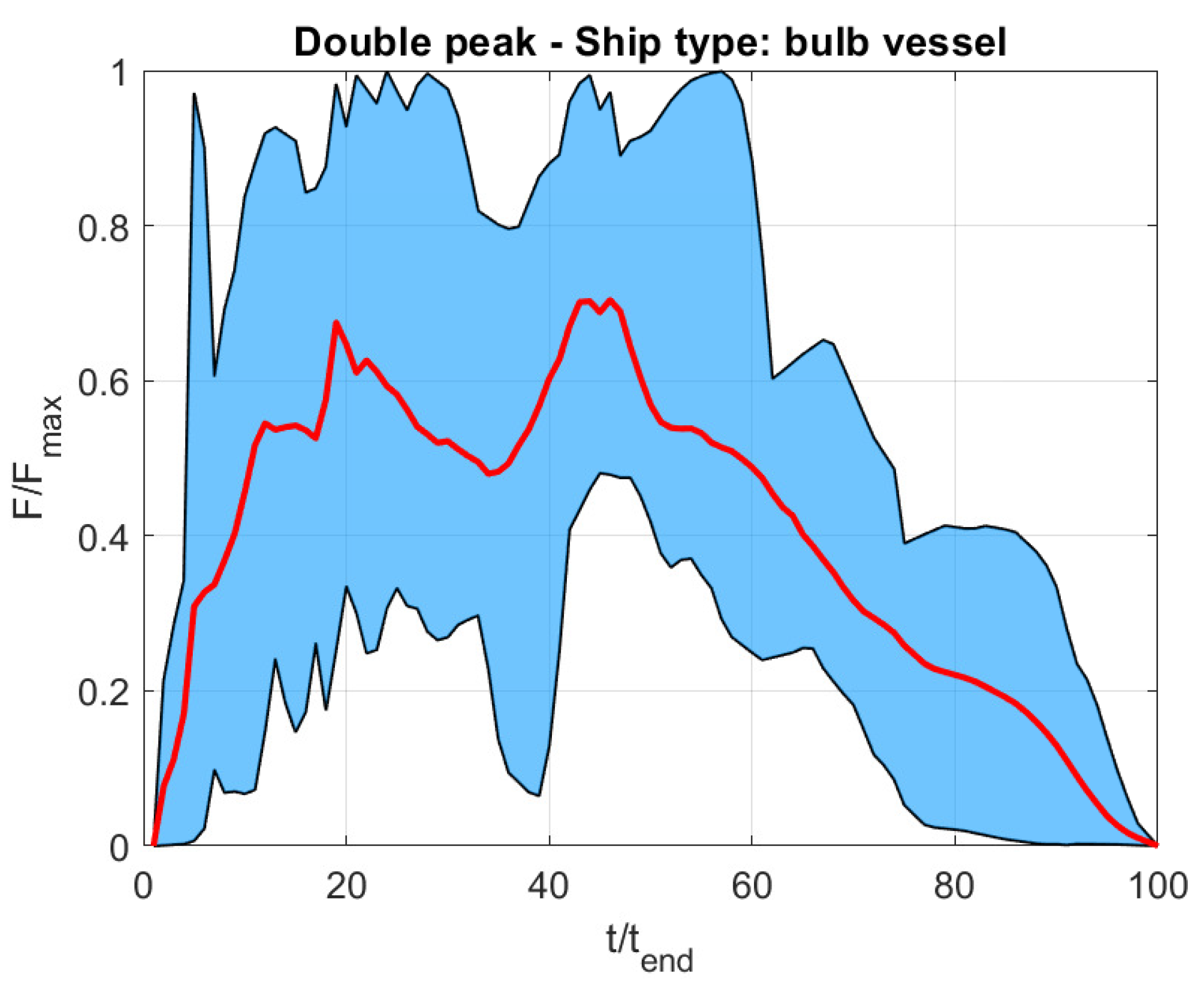
In this work, bulb vessel and barge impacts are investigated, considering specific sub-categories. The result of the clustering action according to the examined literature concerning bulb vessel impacts with a “double-peak” shape force [37,39,42] is presented in Figure 3. Alternatively, for a barge, considering the single peak shaped force only [41,44], the result is shown in Figure 4.
The impact forces are taken from the literature and normalized both in regard to time and peak force. Starting from the impact plot proposed by an author in the literature, the time is divided by the total time duration in order to obtain a normalized time of 1 (). The same process is repeated for the force (). The various forces are then compared to each other to observe if the same pattern is recurrent in different papers. In order to obtain a better understanding of the behavior, an average plot (red curves in Figure 3 and Figure 4) is calculated by averaging all the analyzed plots. A light-blue shaded region around the mean value at each time instant is added considering maximum and minimum values among the different curves, evaluated at each time instant. The obtained graphical representation shows that the selected [41,44] force pattern of a barge impact presents a pronounced peak, followed by a rapidly decreasing trend. The force pattern associated with the selected [37,39,42] bulb vessel impact shows more maxima, coupled with a longer duration of the high force level. A comparison between the two representative force patterns indicates that the barge impact force is more impulse-like. All the chosen impact forces refer to papers where they were obtained from an FEM simulation that models a vessel impacting a bridge or a pier. Scenarios that involve rigid walls or other types of experiments are not included in the clustering process in order to reduce variability.
3. Models and Scenarios
3.1. Impact Forces
A set of the forces presented in the previous section was sampled at 50 Hz and used as input for dynamic simulations. The impact forces were scaled in terms of magnitude from 5 to 40 MN to investigate a wide loading scenario.
The set of considered forces is composed as follows:
It is worth noting that Figure 3 and Figure 4 show the general shape of the considered sub-categories of bulb vessel and barge impact forces, smoothed via the envelope process. For the time integration of bridge and train responses, it is necessary to adopt a single time history that is not smoothed.
3.2. Bridge Model
For the purpose of this work, a bridge representative of the typical configuration was considered. It is featured by a continuous deck that increases the structural interaction between adjacent spans. The main characteristics of the bridge FEM model, which consists of a unifilar beam model (see Figure 7), are collected in Table 1. Each beam element, composing the bridge deck or pier, is defined by equivalent sectional properties. The bridge deck presents a unique cross-section, shown in Figure 8, which is kept constant along its entire length. Moreover, each pier, the geometrical properties of which are reported in Table 1, is characterized by a constant cross-section from the foundation level to support bearings. Pier foundations are modeled by means of linear springs that connect the bottom of each pier to the ground. The stiffness values of foundations are derived from the studied literature and collected in Table 2. These values are also compared with those derived by Xia et al. [23,28], who provide information about two different bridge typologies. It is important to remark that according to Jensen et al. [27], the foundation stiffness can vary by a factor of in modulus due to different soil conditions (e.g., very stiff, weak, very weak).
The connection between the deck and the pier is realized through steel bearings, representing a widespread solution for this type of bridge [23]. The model of bearing connections is based on equivalent linear springs and dampers that constrain the deck only in the lateral and vertical directions. The entire continuous deck is restrained along the longitudinal direction at one end on the ground.
To correlate train and bridge dynamics, the first modes of the bridge structure were calculated, shown in Figure 9, while the associated eigenfrequencies are collected in Table 1. Except for 0.74 Hz (the second mode), the presented natural frequencies are associated with the lateral mode shapes that appear to be predominant in the bridge response due to ship impact evaluated at deck level, as shown in Section 4.
The track system is considered to be rigidly connected with the bridge deck; the simulations were all carried out considering track geometrical irregularities that, as shown in Figure 10, consist of three distinct components, namely vertical ( = 5.4 mm), lateral ( = 2.8 mm) and cross-level ( = 1.4 mrad) irregularities. The adopted geometrical track irregularity components were extracted from the respective PSD functions reported in [49].
3.3. Train Model
A double-deck train is employed in the simulations, and its configuration is reported in Table 3, where H represents the head coach, T the trailer coach and M the motorized coach. Each coach of the train is represented by a multi-body model (see Figure 11) with 35 degrees of freedom (5 dofs for each bogie, car body and wheel set), with primary and secondary suspensions modeled by means of linear spring elements and dampers. Since, in the event of a ship collision, consistent lateral dynamics are involved, lateral bumpstops are inserted between the bogie and the coach, modeled through non-linear restraining forces (see Figure 12b). The purpose of the bumpstop is to limit the relative lateral displacement between the bogie frame and the car body in the presence of high lateral inertial forces associated with lateral and roll acceleration of the car body. The relationship between the bumstop force and the relative displacement has a first interval with zero force in order to avoid lateral force transmission between the bogie frame and the car body for small relative movements. A continuous action of the bumpstop between the car body and bogie would have a detrimental effect on the comfort of the passengers during normal operating conditions. After the zero force interval, the bumstop force presents an increasing stiffness pattern. This vehicle component introduces a strong non-linearity into the system that is activated in the case of large relative lateral displacements between the car body and bogies, which may occur as a consequence of ship collision events.
The main train mechanical parameters are reported in detail in Table A1 in the Appendix A, while the train structure together with the first natural frequencies involving the car body are collected in Table 3.
3.4. Safety Coefficients
The forces exchanged between the wheels and rails (see Figure 12a) play a fundamental role in rail vehicle dynamics, and, in the scenarios considered in the paper, they are even more important, since thet are fundamental in the calculation of running safety coefficients. According to standards [50,51], the evaluation indices for running safety include derailment and unloading coefficients. According to EN14363 [50], the derailment coefficient and its threshold are defined as follows:
where Y and Q are, respectively, the lateral and vertical components of the contact forces exchanged between the wheel and rail at the contact point (see Figure 12). The threshold limit is set to 1.2 (or 120%) if the train is running along a straight trajectory (present case), while it is limited to 0.8 (or 80%) when the train travels along a curve.
According to EN14067-6 [51], the unloading factor is defined as follows:
where Q is the vertical contact force and is the wheel static vertical load. The unloading limit is set to 0.9 for both curved and straight lines. As suggested by the formula, this coefficient quantitatively evaluates the dynamic variation in vertical contact forces with respect to the static values when wheel uplift occurs (i.e., ); the unloading coefficient related to that wheel assumes a unitary value, which represents the limit of the physical value.
3.5. Wheel–Rail Contact Profiles
The two sub-systems, the train on one side and the track and bridge on the other, interact through the contact forces exchanged at each wheel–rail contact point. The modeling of wheel–rail contacts is of particular importance when examining running conditions close to the limits, as they are the connection between the local and global aspects of the runability problem. The evaluation of the contact is based on the transversal profiles of the wheel and the rail. Coupling them enables the generation of a table of geometrical parameters as a function of the relative lateral wheel set–rail displacement. The main geometrical parameters considered are the rolling radius of the wheel, the contact angle, and the local radius of curvatures of the profiles in contact as a function of relative wheel set–track lateral displacement. This preliminary geometrical analysis takes into account the possible existence of multiple contact conditions, creating lookup tables for each geometrical parameter.
Figure 13 shows the variation in the rolling radius, with respect to the nominal one, of the coupling between new wheel (ORE S1002) and rail (UIC 60) profiles, with a 1:20 rail inclination. Each colored branch corresponds to a contact zone on the wheel profile, as shown in Figure 14. Moving from the centered wheel set position towards the contact on the flange, the location of the contact point migrates from the thread (blue circles) to the throat (red circles) and finally to the flange (green circles). The contact zones are not continuous, the dislocation from one zone to the other corresponds to the “jumps” in the diagram of the rolling radius, creating separate branches. These branches have some degree of superposition so that multiple contact point conditions can be managed.
With the development of wear, the wheel and the rail profiles change, and this has an important impact on the functions that describe the geometrical parameters. Figure 15 is the same representation in Figure 13, but considering moderate wear of the wheel and rail profile, thus leading to an equivalent conicity of 0.15. As will be shown in the simulation analysis, this has an impact on the dynamics of wheel set–track interaction following the ship impact.
During the simulation in the time domain, the wheel–rail contact normal forces are computed at each integration step through a multi-Hertzian approach [52]. Subsequently, the longitudinal and transversal creepage forces are calculated according to the Shen–Hedrick–Elkins creepage dependence formulation [53]. Iterations are carried out at each integration time step to converge to a congruent and balanced solution, as described in the following section.
3.6. TBI Time Integration Procedure
Train–track–structure dynamic interactions were simulated through ADTReS software. The latter is a simulation software developed internally (across several decades) and based on Fortran code for train–track–structure dynamic interaction simulations [1,54]. In ADTReS software, the structure (FE approach) and vehicles (multibody approach) are treated as two different sub-systems, mathematically modeled with two different equations. Concerning the structure, the matrix formulation of the equation of motion is organized as follows:
where , and represent, respectively, the mass, damping and stiffness matrices of the structure, and is the vector containing the structure’s free coordinates (the structure’s degrees of freedom). is the column vector of the generalized contact forces, which are defined according to the structure and the vehicle’s free coordinates. In addition, stands for the action of other external forces, i.e., the ship impact force in this work.
Instead, for each i-th vehicle, the following matrix formulation of the equation of motion is considered:
where , and stand for the mass, damping and stiffness matrices of the i-th vehicle, and is the vector collecting the i-th vehicle’s free coordinates (the i-th vehicle’s degrees of freedom). is the column vector of the generalized contact forces, while considers non-linear suspension components, such as bumpstop elements. Finally, the vector accounts for external forces, such as wind forces, acting on the vehicle.
It is now clear that, as mentioned in the previous section, the two sub-systems (structure and vehicle) are dynamically coupled through contact forces.
Concerning generalized contact force computations, in Equations (3) and (4), for each vehicle, the displacements and velocities of the contact points on the rail and wheel must be computed. From these, contact forces are derived, as they are functions of the wheel and rail motion at the contact point. Subsequently, generalized contact forces acting on the structure and vehicle are calculated.
Assuming a forward motion of the rail vehicle, with a constant travelling speed V, the longitudinal position of the k-th wheel along the generic p-th finite element is defined as follows:
where is the initial position of the k-th wheel, while is the position of the first node of the p-th beam finite element on which the wheel is running. Once the positions and velocities of contact points at are defined, it is possible to obtain the components of the contact forces exchanged between the track and wheels. As mentioned in Section 3.5, the wheel–rail contact model is based on a preliminary geometrical analysis through pre-computation of geometrical parameters, such as the contact angle or local radii of curvature, expressed as functions of the wheel–rail relative position. Once the contact forces are computed for each activated contact point (refer to Section 3.5), they are projected onto the global reference system and finally assembled into the generalized forces vectors [1,54].
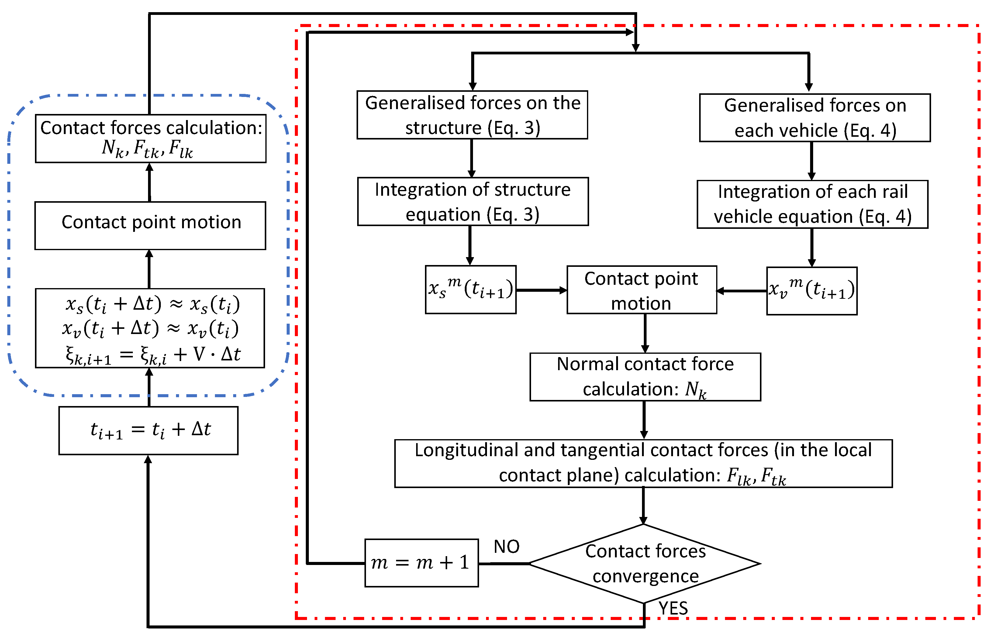
Equations (3) and (4) are integrated in the time domain according to the procedure schematically depicted in Figure 16. In particular, at the beginning of the generic i-th time step, the first approximation (m = 1) of the contact point motion is calculated, considering the wheels in the new position. Once the contact forces are calculated, after having computed the generalized contact forces, Equations (3) and (4) are integrated. Then, a new approximation (m = m + 1) of the contact point motion is obtained and the contact forces are calculated again. Therefore, an iterative procedure is devised (red box in Figure 16) within the i-th time step; after convergence is reached for the contact forces, the time step can be incremented. Time integration is performed through the Newmark method [54].
4. Structural Response to Ship Impact Events
After the ship impact occurs, the bridge starts to vibrate, thus affecting the dynamics of the train. The impact forces (see Figure 5 and Figure 6) have been scaled from a peak value of 5 MN up to 40 MN. The upper limit is set according to Xia et al. [23], who used a linear elastic bridge model up to a peak force of 40 MN without losing accuracy. The primary consequences above this impact limit are plastic deformation of the foundation and possible structural damage around the impact zone that cannot be further neglected due to significant variations in the global behavior of the bridge. Several simulations were performed in this work in order to deeply investigate the role played by a number of operational factors on train running safety in the presence of a ship impact. The aspects investigated are the following:
- The effect of the travelling speed.
- The effect of the type of impact force due to barge and bulb vessel collisions. Their magnitude is scaled from 5 MN to 40 MN.
- The effect of the wheel–rail contact profile. An analysis is conducted considering new and moderately worn wheel–rail contact profiles.
All the results presented in this section regard the case of a ship impact occurring at the central bridge pier (see Figure 7), when the first coach’s center of mass is at the impacted pier. This section aims to present the effects of ship collisions on bridge motion. Subsequently, in the next section, the focus is moved to the analysis of train dynamics and running safety.
Considering the case of a barge impact, modeled by the force–time function shown in Figure 5 with a peak value of 40 MN, the structure lateral displacements are shown in the top left of Figure 17 and the accelerations are shown in the same figure in the bottom left position. Each diagram reports the impact point (level z = 13 m) and the foundation (level z = 0 m) responses corresponding to the impacted pier. On the right, the corresponding spectral analysis is reported for each time series. The peak values of displacement are close to each other (around 35–40 mm), while a more pronounced oscillation decay (i.e., a higher oscillation amplitude) is visible at the impact point level (red line). Lateral acceleration at the same points, dominated by higher frequencies, is very close, with a peak value around 8.75 m/s2.
In order to show the global participation of the structure, Figure 18 reports the lateral displacement and acceleration of the deck (level z = 38 m) corresponding to the impacted pier (x = 240 m) and the adjacent midspans (x = 200, 280 m). From the top-left diagram of Figure 18, a maximum displacement value of about 56 mm can be observed; in the spectral analysis on the right, it is possible to observe two peaks corresponding to the first and third lateral bridge frequencies (at 0.47 Hz and 1.33 Hz). From the left-bottom diagram of Figure 18, an acceleration peak about 2.3 m/s2 was found in the deck section, in correspondence with the impacted pier (x = 240 m). These values (accelerations and displacements) are comparable to cases in which the bridge structure is subject to earthquake events [4,5,9]. It is worth pointing out that the displacement peak at the deck level is higher than that at the impact point due to the contribution of the rotation and flexural deflection of the pier, while the deck accelerations are remarkably lower than those at the impact point, as higher modes are involved at the impact point.
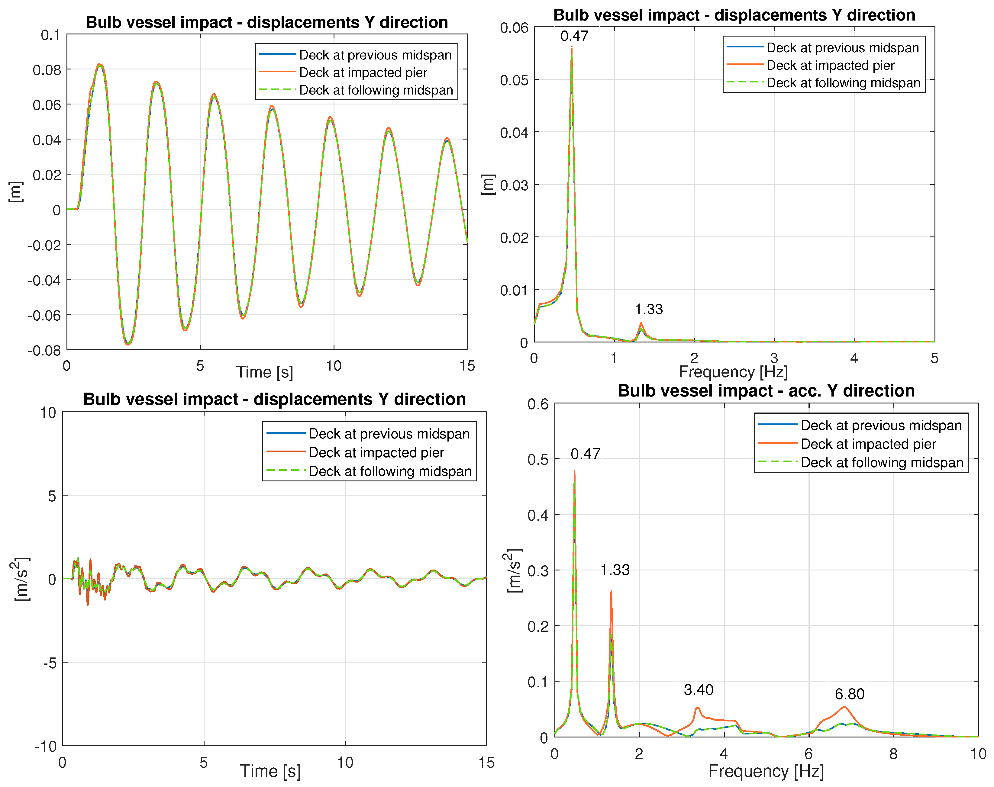
Considering now the case of a bulb vessel impact (see Figure 6), again with a maximum peak value of 40 MN, the structure lateral displacements and accelerations (and relative spectra, on the right) at the impact point (z = 13 m) and foundation (z = 0 m) level corresponding to the impacted pier are shown in Figure 19. An acceleration peak of ≈10 m/s2 was found at the foundation level (z = 0 m). From the top-left diagram in Figure 19, a maximum lateral displacement of 43 mm is caused by the collision at the impacted point, while on the right, it is possible to observe two peaks, again corresponding to the first and third lateral bridge frequencies, similarly to what was found in the barge impact case. The deck motion is shown in Figure 20 which reports the lateral displacement and acceleration of the deck corresponding to the impacted pier (x = 240 m) and the adjacent midspans (x = 200, 280 m). The maximum lateral displacement value of the deck is around 83 mm, larger than that found for the barge impact (56 mm). The lateral acceleration peak at the deck level is lower than 2 m/s2 (≈1.6 m/s2) in correspondence with the impacted pier (x = 240 m).
It can be concluded that the bulb vessel impact tends to involve the first lateral mode of the bridge structure, while the barge impact, more resembling an impulse-like shape, tends to also excite the higher modes. In fact, when comparing the spectra in Figure 18 (bottom right) for barge impact with the spectra in Figure 20 (bottom right) for bulb vessel impact, it can be observed that the barge impact tends to excite the higher frequencies (1.33 and 3.33 Hz) more with respect to the bulb vessel impact. Again, this can be justified by the impulse-like shape of the barge impact force.
5. Train Running Safety Coefficients
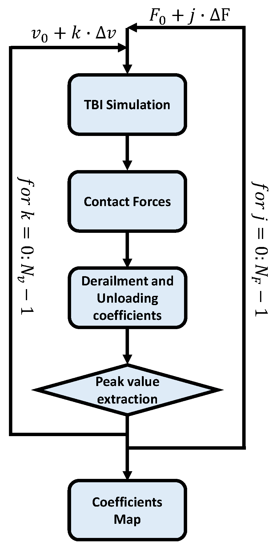
The focus is now moved to train running safety. This section initially shows examples of time series of wheel–rail contact forces to show step by step how the final maps are built. The procedure followed to shift from contact force components to the final safety coefficient maps is schematically depicted in Figure 21. A set of TBI simulations was performed, considering different travelling speeds () and force peaks (). For each combination of the these two parameters, TBI simulations were run; subsequently, contact force components were downloaded for each wheel set of the vehicle (for left and right wheels). Starting from these, safety coefficients were computed in compliance with [50,51]. Finally, peaks were extracted in terms of derailment and unloading coefficients considering all wheels. This entire process was repeated for each combination of vehicle speed and collision force peak magnitude.
Considering as an example the case of a barge impact with the train running at 150 km/h, Figure 22 shows the resulting vertical (Q) and lateral (Y) contact forces of the left and right wheels for wheel set N. 18. The examined wheel set enters the bridge once the lateral motion of the deck is already initiated by the ship impact. As a consequence, a pattern with alternate loading–unloading cycles between the left (red line) and right (blue line) wheels appears for the vertical Q forces. The lateral Y forces exhibit peaks corresponding to the occurrence of wheel flange contact with the rail, with the same period as the vertical loading–unloading cycles. The geometry of wheel–rail contacts, which is highly non-linear, is reflected in the appearance of the peaks in the Y forces. As an additional remark, the peak values of the lateral Y forces appear both on the left and on the right wheel, indicating that the wheel set is moving in both directions after the ship impact, and it is contained only by the flange contact. Exceeding the lateral force would increase the probability of derailment. The derailment and unloading safety coefficients, calculated from the previously reported contact forces, are plotted in Figure 23. The derailment coefficients show a peak in correspondence with the occurrence of peak (positive or negative) values of the Y force, while the unloading coefficient reaches the local maximum with a smoother trend, as it is related to the oscillation associated with the combined lateral–rolling low-frequency motions of the car body.
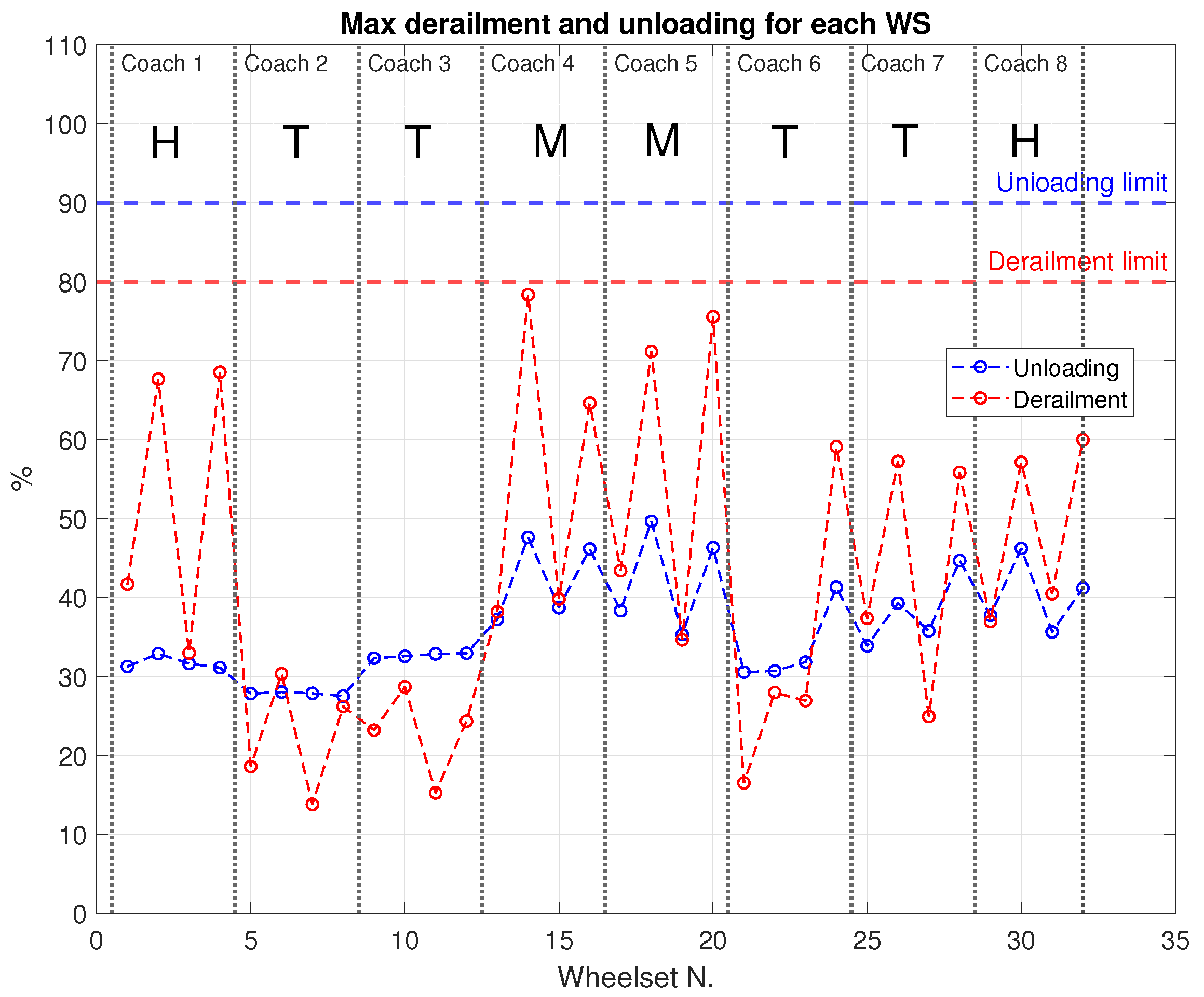
Taking now the absolute maximum value of the safety coefficients for each wheel set, an overall view of the entire train can be obtained, as shown in Figure 24. It can be observed that the derailment coefficients tend to be higher for head (H) and motor (M) coaches, while a more balanced situation is obtained for the unloading coefficient. The final level of analysis concerns the distribution of the maximum safety coefficients as a function of the train speed and impact intensity, included in a safety map representation (see Figure 25 and Figure 26). The maps collect the maximum value of each safety coefficient from all the wheel sets of the train, considering the input force magnitude and train speed as parameters. The map was built through a massive set of simulations for a given wheel–rail contact profile. Black dashed lines are used to represent different iso-level lines, which define different regions in terms of safety coefficient values. This means that, for instance, considering the derailment coefficient map, the region between level lines 60 and 70 will represent scenarios in which the maximum derailment coefficients are all contained in the range of 60 to 70%. The shape of the maps in Figure 25 and Figure 26 reveals somewhat different sensitivities to the peak load and train speed in the considered speed and loading ranges.
The maps in Figure 25 refer to a barge impact, where the two maps on the left show the derailment (top) and unloading (bottom) peak coefficients for the new wheel–rail profile. The same kind of maps are reported on the right, but are related to the moderately worn wheel–rail profile considered in this paper. A region with a 70% derailment index appears only for new wheel profiles between speeds of 35 m/s and 60 m/s. Moving within the map from left to right (i.e., an increasing train speed), there is a dependence on speed in the lower range of the impact force, which is more pronounced for the worn profile. In the higher range of impact force magnitude, the iso-lines are almost parallel to the train speed axis, indicating a weak dependence on train speed. On the other hand, considering the unloading coefficients, the maps for the new and worn wheel–rail profiles are very similar. This appears to be consistent with the fact that unloading is mainly dependent on the car body motion, while derailment is also related to the geometry of the wheel–rail profile, which can act as an impacting parameter. In other words, unloading is less dependent on wheel–rail contact non-linearities than derailment. In Figure 25 and Figure 26, an area with higher derailment coefficients is found for the new wheel–rail profiles.
Similar observations are noted for the scenarios depicted in Figure 26, which refer to the case of a bulb vessel collision. A more favorable behavior in terms of derailment coefficients is found when dealing with a worn profile (right side of Figure 25 and Figure 26) than with a new profile (left side of Figure 25 and Figure 26). The main reason can be attributed to the larger equivalent conicity of the wheel–rail profile coupling, which moves from 0.05 for the new profiles to 0.15 for the worn ones. The increase in the equivalent conicity increases the geometrical guidance action and helps to reduce the transversal displacement of the wheel set inside the track. As a result, the wheel set tends to remain more centered inside the track, reducing the occurrence of flange contacts. It is worth recalling that a too-high conicity (above 0.2) has a negative effect, causing a decrease in the critical speed of the train. Comparing the four investigated scenarios (barge and bulb vessel collisions with new and moderately worn profiles), it is possible to observe that, except for the derailment coefficient map when a worn profile is considered, higher safety coefficients are obtained when a bulb collision is considered compared to a barge impact. An important aspect that may be pointed out in Figure 25 and Figure 26 is that the train speed plays a role in the lower and higher ranges of impact force for the derailment coefficient, which is not monotonically related to the increase in train speed. This confirms what was observed in [29]. As for the unloading coefficients, speed has an influence at a low impact force and less influence at higher levels impact force.
6. Conclusions
This work presented a numerical analysis of the dynamic train–bridge interactions after ship collision events occurring at the pier level. The objective of the paper was to investigate train running behavior in the presence of ship impact events as a function of different operational factors, such as ship typology, impact intensity, travelling speed, and the geometry of the wheel–rail contact profile. For this purpose, a double-deck train travelling at different speeds, two types of ship impacts (i.e., a barge and a bulb vessel) with scaled intensities (from 5 MN to 40 MN), and, finally, two types of wheel–rail profiles (new and moderately worn) were studied. The investigation was carried out through time-domain numerical simulations of train–bridge interactions, considering the impact force as a time-dependent function. Train dynamics were examined by means of derailment and unloading safety coefficients, defining maps for the maximum value of safety running coefficients as a function of the train speed and the magnitude of impact force. The results of the simulations led to the following conclusions:
- Bulb vessel impacts were found to be a more critical scenario for both wheel–rail profiles (i.e., new and worn) in terms of train running safety. In fact, the resulting safety maps highlighted larger areas of higher values of derailment and unloading coefficients in the case of a bulb vessel collision with the central pier of a bridge than in the case of barge impact. This is caused by the difference in the impact force–time function of the two types of vessels (a barge and a bulb vessel).
- The derailment coefficient is more sensitive to train speed, especially in the extreme ranges of impact forces, considering that the highest safety coefficients are not necessarily found at the maximum train speed.
- The unloading coefficient is predominantly sensitive to the magnitude of the impact force and less dependent on the train speed.
- The wheel–rail contact geometry can significantly affect the train dynamic response and the running safety after a ship impact. Due to the increased conicity, moderately worn wheels (0.15 was examined) tend to limit the motion of the wheel set inside the track, also improving the running safety in the region of high impact forces. In this respect, simulations with new wheel and rail profiles are more demanding than those with a worn profile.
A limitation of this work is represented by the consideration of ideally linear foundations with fully elastic stiffness elements. Adopting non-linear foundations would allow for the investigation of more critical scenarios featured by higher impact forces to study the effect of permanent displacement of bridge foundations, piers, and the deck on train running safety. Moreover, another proposed future work is the exploration of train running safety in the case of empty and fully loaded freight trains.
Author Contributions
Conceptualization L.B and A.C.; simulations G.S.; data curation G.S. and L.B.; writing—original draft G.S.; writing—review and editing L.B., A.C. and G.S.; supervision A.C. and L.B. All authors have read and agreed to the published version of the manuscript.
Funding
This research received no external funding.
Data Availability Statement
Data are unavailable due to privacy.
Conflicts of Interest
The authors declare no conflicts of interest.
Appendix A
Table A1 shows the main mechanical parameters of the train used in this work.

Table A1.
Main mechanical parameters of the adopted train model.
| H, M | T | u.m. | |
|---|---|---|---|
| Car body | |||
| Mass | 45,000 | 52,800 | kg |
| Yaw moment of inertia | 2.25 | 2.64 | kg·m2 |
| Pitch moment of inertia | 2.35 | 2.76 | kg·m2 |
| Roll moment of inertia | 1.40 | 1.64 | kg·m2 |
| Bogie | |||
| Mass | 4.50 | 4.20 | kg |
| Yaw moment of inertia | 7.25 | 6.77 | kg·m2 |
| Pitch moment of inertia | 8.55 | 7.98 | kg·m2 |
| Roll moment of inertia | 3.36 | 3.14 | kg·m2 |
| Primary vertical stiffness | 2.86 | 3.00 | N/m |
| Primary lateral stiffness | 2.00 | 2.00 | N/m |
| Primary vertical damping | 3.44 | 3.44 | N·s/m |
| Lateral axle-box damping | 6.70 | 6.70 | N·s/m |
| Secondary vertical stiffness | 1.01 | 1.01 | N/m |
| Secondary lateral stiffness | 3.20 | 3.70 | N/m |
| Torsion bar stiffness | 3.40 | 3.40 | N/rad |
| Secondary vertical damping | 3.15 | 3.70 | N·s/m |
| Secondary lateral damping | 1.70 | 2.42 | N·s/m |
| Yaw damping | 8.00 | 8.00 | N·s/rad |
| Wheel set | |||
| Mass | 2000 | 1500 | kg |
| Wheelbase | 2.3 | 2.5 | m |
References
- Bruni, S.; Collina, A.; Corradi, R.; Diana, G. Numerical simulation of train-track-bridge dynamic interaction. In Computational Mechanics, Proceedings; Tsinghua University Press: Beijing, China, 2004; pp. 237–242. [Google Scholar]
- Heleno, R.; Montenegro, P.; Carvalho, H.; Ribeiro, D.; Calcada, R.; Baker, C. Influence of the railway vehicle properties in the running safety against crosswinds. J. Wind Eng. Ind. Aerodyn. 2021, 217, 104732. [Google Scholar] [CrossRef]
- He, X.; Kawatani, M.; Hayashikawa, T.; Matsumoto, T. Numerical analysis on seismic response of Shinkansen bridge-train interaction system under moderate earthquakes. Earthq. Eng. Eng. Vib. 2011, 10, 85–97. [Google Scholar] [CrossRef]
- Yang, X.; Wang, H.; Jin, X. Numerical Analysis of a Train-Bridge System Subjected to Earthquake and Running Safety Evaluation of Moving Train. Shock Vib. 2016, 2016, 9027054. [Google Scholar] [CrossRef]
- Jin, Z.; Pei, S.; Li, X.; Liu, H.; Qiang, S. Effect of vertical ground motion on earthquake-induced derailment of railway vehicles over simply-supported bridges. J. Sound Vib. 2016, 383, 277–294. [Google Scholar] [CrossRef]
- Zeng, Q.; Dimitrakopoulos, E.G. Derailment mechanism of trains running over bridges during strong earthquakes. Procedia Eng. 2017, 199, 2633–2638. [Google Scholar] [CrossRef]
- Zeng, Q.; Dimitrakopoulos, E.G. Vehicle–bridge interaction analysis modeling derailment during earthquakes. Nonlinear Dyn. 2018, 93, 2315–2337. [Google Scholar] [CrossRef]
- Wu, X.; Liang, S.; Chi, M. An investigation of rocking derailment of railway vehicles under the earthquake excitation. Eng. Fail. Anal. 2020, 117, 104913. [Google Scholar] [CrossRef]
- Goto, K.; Sogabe, M.; Tokunaga, M. Evaluation of vehicle running safety on railway Structures during earthquake. Int. J. Transp. Dev. Integr. 2020, 4, 113–128. [Google Scholar] [CrossRef]
- Jin, Z.; Liu, W.; Pei, S. Probabilistic evaluation of railway vehicle’s safety on bridges under random earthquake and track irregularity excitations. Eng. Struct. 2022, 266, 114527. [Google Scholar] [CrossRef]
- Guo, J.; He, J. Dynamic response analysis of ship-bridge collisions experiment. J. Zhejiang Univ.-Sci. A 2020, 21, 525–534. [Google Scholar] [CrossRef]
- Fan, W.; Sun, Y.; Yang, C.; Sun, W.; He, Y. Assessing the response and fragility of concrete bridges under multi-hazard effect of vessel impact and corrosion. Eng. Struct. 2020, 225, 111279. [Google Scholar] [CrossRef]
- Wang, J.; Yan, H.; Qian, H. Comparisons of Ship Collision Design Formula for Bridges Based on FEM Simulations. J. Highw. Transp. Res. Dev. 2006, 1, 46–50. [Google Scholar] [CrossRef]
- Fan, W.; Liu, Y.; Liu, B.; Guo, W. Dynamic Ship-Impact Load on Bridge Structures Emphasizing Shock Spectrum Approximation. J. Bridge Eng. 2016, 21. [Google Scholar] [CrossRef]
- Wan, Y.; Zhu, L.; Fang, H.; Liu, W.; Mao, Y. Experimental testing and numerical simulations of ship impact on axially loaded reinforced concrete piers. Int. J. Impact Eng. 2019, 125, 246–262. [Google Scholar] [CrossRef]
- Consolazio, G.R.; Cowan, D.R. Numerically Efficient Dynamic Analysis of Barge Collisions with Bridge Piers. J. Struct. Eng. 2005, 131, 1256–1266. [Google Scholar] [CrossRef]
- Zhu, L.; Liu, W.; Fang, H.; Chen, J.; Zhuang, Y.; Han, J. Design and simulation of innovative foam-filled Lattice Composite Bumper System for bridge protection in ship collisions. Compos. Part B Eng. 2019, 157, 24–35. [Google Scholar] [CrossRef]
- Guo, X.; Zhang, C.; Chen, Z. Dynamic performance and damage evaluation of a scoured double-pylon cable-stayed bridge under ship impact. Eng. Struct. 2020, 216, 110772. [Google Scholar] [CrossRef]
- Tao, F.; Xiaoqian, R.; Kai, W. Vessel-Bridge Collision Reliability Assessment Based on Structural Dynamic Analysis. Adv. Civ. Eng. 2021, 2021, 5929019. [Google Scholar] [CrossRef]
- Song, Y.; Wang, J. Development of the impact force time-history for determining the responses of bridges subjected to ship collisions. Ocean Eng. 2019, 187, 106182. [Google Scholar] [CrossRef]
- Sha, Y.; Amdahl, J.; Dørum, C. Numerical and analytical studies of ship deckhouse impact with steel and RC bridge girders. Eng. Struct. 2021, 234, 111868. [Google Scholar] [CrossRef]
- Sha, Y.; Amdahl, J.; Dørum, C. Dynamic responses of a floating bridge subjected to ship collision load on bridge girders. Procedia Eng. 2017, 199, 2506–2513. [Google Scholar] [CrossRef]
- Xia, C.; Xia, H.; De Roeck, G. Dynamic response of a train-bridge system under collision loads and running safety evaluation of high-speed trains. Comput. Struct. 2014, 140, 23–38. [Google Scholar] [CrossRef]
- Xia, C.; Lei, J.; Zhang, N.; Xia, H.; De Roeck, G. Dynamic analysis of a coupled high-speed train and bridge system subjected to collision load. J. Sound Vib. 2012, 331, 2334–2347. [Google Scholar] [CrossRef]
- Li, P.; Li, Z.; Han, Z.; Zhu, S.; Zhai, W.; Lou, H. Running safety evaluation of high-speed train subject to the impact of floating ice collision on bridge piers. Proc. Inst. Mech. Eng. Part F J. Rail Rapid Transit 2022, 236, 220–233. [Google Scholar] [CrossRef]
- Kalajahi, A.R.; Esmaeili, M.; Zakeri, J.A. Dynamic analysis of a coupled high-speed train and bridge system subjected to a sea wave hydrodynamic load. Lat. Am. J. Solids Struct. 2021, 18, e341. [Google Scholar] [CrossRef]
- Jensen, J.L.; Svensson, E.; Eiriksson, H.; Ennemark, F. Ship-induced derailment on a railway bridge. Struct. Eng. Int. 1996, 6, 107–112. [Google Scholar] [CrossRef]
- Xia, C.; Zhang, N.; Xia, H.; Ma, Q.; Wu, X. A framework for carrying out train safety evaluation and vibration analysis of a trussed-arch bridge subjected to vessel collision. Struct. Eng. Mech. Int. J. 2016, 59, 683–701. [Google Scholar] [CrossRef]
- Li, Y.; Deng, J.; Wang, B.; Yu, C. Running Safety of Trains under Vessel-Bridge Collision. Shock Vib. 2015, 2015, 252574. [Google Scholar] [CrossRef]
- Zhang, J.; Zhang, Z.; Zhu, Z.; Liu, D.; Li, X. Train-Track-Bridge coupling vibration and train running safety under vessel impact. J. Vib. Control 2023. [Google Scholar] [CrossRef]
- Gong, K.; Liu, L.; Yu, C.; Wang, C. Train derailment process analysis on heavy haul railway bridge under Ship impact. Symmetry 2021, 13, 2122. [Google Scholar] [CrossRef]
- Xia, C.; Ma, J.; Xia, H. Dynamic analysis of a train-bridge system to vessel collision and running safety of high-speed trains. Vibroeng. Procedia 2015, 5, 509–514. [Google Scholar]
- AbuBakar, A.; Dow, R. The impact analysis characteristics of a ship’s bow during collisions. Eng. Fail. Anal. 2019, 100, 492–511. [Google Scholar] [CrossRef]
- Fan, W.; Yuan, W.; Chen, B. Steel Fender Limitations and Improvements for Bridge Protection in Ship Collisions. J. Bridge Eng. 2015, 20. [Google Scholar] [CrossRef]
- Yang, L.; Liu, J. A study on ship impacting a flexible crashworthy device for protecting bridge pier. EPJ Web Conf. 2015, 94, 01059. [Google Scholar] [CrossRef]
- Chen, G.; Huang, H.; Xiang, Z. Experimental Investigation on the Anticollision Performance of Corrugated Steel-Reinforced Composites for Bridge Piers. Shock Vib. 2021, 2021, 5847559. [Google Scholar] [CrossRef]
- Gholipour, G.; Zhang, C.; Mousavi, A.A. Effects of axial load on nonlinear response of RC columns subjected to lateral impact load: Ship-pier collision. Eng. Fail. Anal. 2018, 91, 397–418. [Google Scholar] [CrossRef]
- Gholipour, G.; Zhang, C.; Mousavi, A.A. Nonlinear failure analysis of bridge pier subjected to vessel impact combined with blast loads. Ocean Eng. 2021, 234, 109209. [Google Scholar] [CrossRef]
- Gholipour, G.; Zhang, C.; Mousavi, A.A. Nonlinear numerical analysis and progressive damage assessment of a cable-stayed bridge pier subjected to ship collision. Mar. Struct. 2020, 69, 102662. [Google Scholar] [CrossRef]
- Sha, Y.; Amdahl, J. Numerical investigations of a prestressed pontoon wall subjected to ship collision loads. Ocean Eng. 2019, 172, 234–244. [Google Scholar] [CrossRef]
- Gholipour, G.; Zhang, C.; Mousavi, A.A. Analysis of girder bridge pier subjected to barge collision considering the superstructure interactions: The case study of a multiple-pier bridge system. Struct. Infrastruct. Eng. 2019, 15, 392–412. [Google Scholar] [CrossRef]
- Fan, W.; Zhang, Z.; Huang, X.; Sun, W. A simplified method to efficiently design steel fenders subjected to vessel head-on collisions. Mar. Struct. 2020, 74, 102840. [Google Scholar] [CrossRef]
- Jiang, P.; Wang, P.; Cao, H.; Wang, F. Research on New Flexible Bridge Pier Anti-collision Technology. IOP Conf. Ser. Earth Environ. Sci. 2020, 565, 1291. [Google Scholar] [CrossRef]
- McVay, M.C.; Wasman, S.J.; Consolazio, G.R.; Bullock, P.J.; Cowan, D.G.; Bollmann, H.T. Dynamic Soil-Structure Interaction of Bridge Substructure Subject to Vessel Impact. J. Bridge Eng. 2009, 14, 7–16. [Google Scholar] [CrossRef]
- Peng, K. Dynamic Ship-bridge Collision Risk Decision Method Based on Time-Dependent AASHTO Model. J. Inst. Eng. (India) Ser. A 2021, 102, 305–313. [Google Scholar] [CrossRef]
- Jilun, M.; Chuang, C.; Shengxie, X. Evaluation on Risk for Ship Collision with Archbridge and Crash Capability of Anti-Collision. Open Civ. Eng. J. 2014, 8, 351–359. [Google Scholar] [CrossRef]
- Fan, W.; Yuan, W. Ship Bow Force-Deformation Curves for Ship-Impact Demand of Bridges considering Effect of Pile-Cap Depth. Shock Vib. 2014, 2014, 201425. [Google Scholar] [CrossRef]
- Fan, W.; Yuan, W. A Simple Procedure for Determination of the Dynamic Ship-Impact Load on Bridge Structures; WIT Press: Billerica, MA, USA, 2014; Volume 141, pp. 73–85. [Google Scholar] [CrossRef]
- ORE B176; Bogies with Steered or Steering Wheelsets. Report No. 1: Specifications and Preliminary Studies, Vol. 2, Specification for a Bogie with Improved Curving Characteristics. ORE: Utrecht, The Netherlands, 1989.
- EN14363; Railway Applications—Testing and Simulation for the Acceptance of Running Characteristics of Railway Vehicles—Running Behaviour and Stationary Tests. CEN: Brussels, Belgium, 2016.
- EN14067-6; Railway Applications—Aerodynamics—Part 6: Requirements and Test Procedures for Cross Wind Assessment. CEN: Brussels, Belgium, 2010.
- Pascal, J.P.; Sany, J.R. Dynamics of an isolated railway wheelset with conformal wheel–rail interactions. Veh. Syst. Dyn. 2019, 57, 1947–1969. [Google Scholar] [CrossRef]
- Shen, Z.Y.; Hedrick, J.K.; Elkins, J.A. A Comparison of Alternative Creep Force Models for Rail Vehicle Dynamic Analysis. Veh. Syst. Dyn. 1983, 12, 79–83. [Google Scholar] [CrossRef]
- Diana, G.; Cheli, F.; Bruni, S. Railway runnability and train-track interaction in long span cable supported bridges. Adv. Struct. Dyn. 2000, 1, 43–54. [Google Scholar]
Figure 1.
Occurrence of peak collision forces in the examined literature [12,13,14,15,16,17,19,33,35,37,38,39,40,41,42,43,44,45,46,47,48]. Most authors focus on investigating impact in a range from 5 to 40 MN as the maximum peak force.
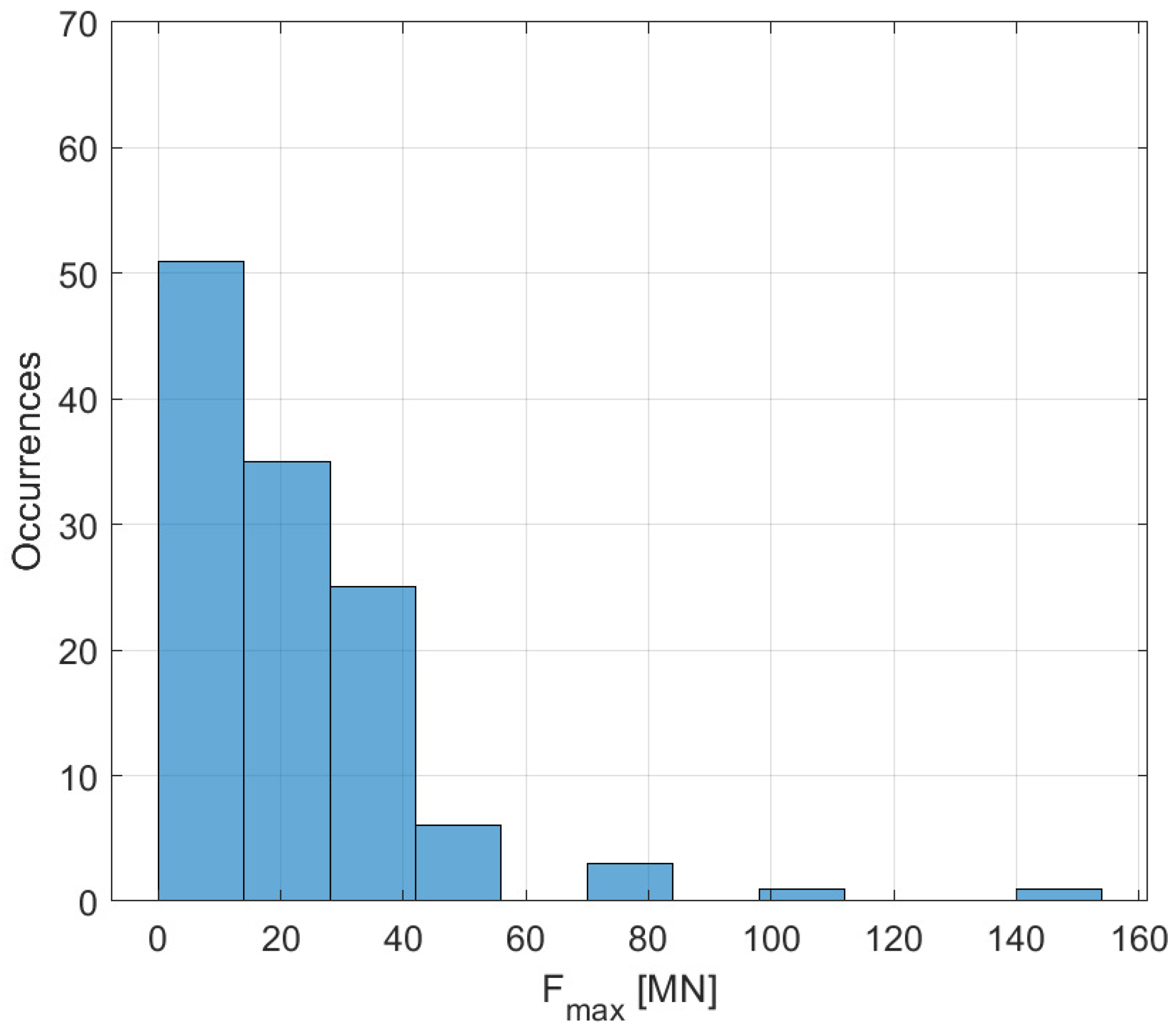
Figure 2.
Occurrence of vessel mass (DWT, ton) in the examined literature [12,13,14,15,16,17,19,33,35,37,38,39,40,41,42,43,44,45,46,47,48]. Most authors focused on investigating vessels below 15,000 DWT (a vessel of this size can reach 150 m in overall length).
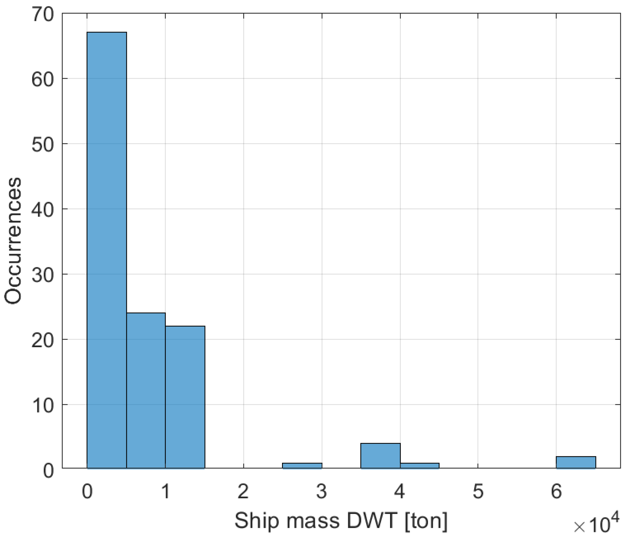
Figure 3.
Impacts involving bulb vessels in the literature with a “double-peak”-shaped time force [37,39,42]. The red line represents the average curve, while the light blue region represents the distribution of force plots around the mean value curve. These impact forces are obtained from an FEM numerical experiment that models an impact between a vessel and a bridge pier.

Figure 4.
Impact forces involving barges from the literature considering a single-peak-shaped force [41,44]. The red line represents the average curve, while the light blue region represents the scatter of force plots around their mean value curve. These impact forces are obtained from an FEM experiment that models an impact between a vessel and a bridge pier.
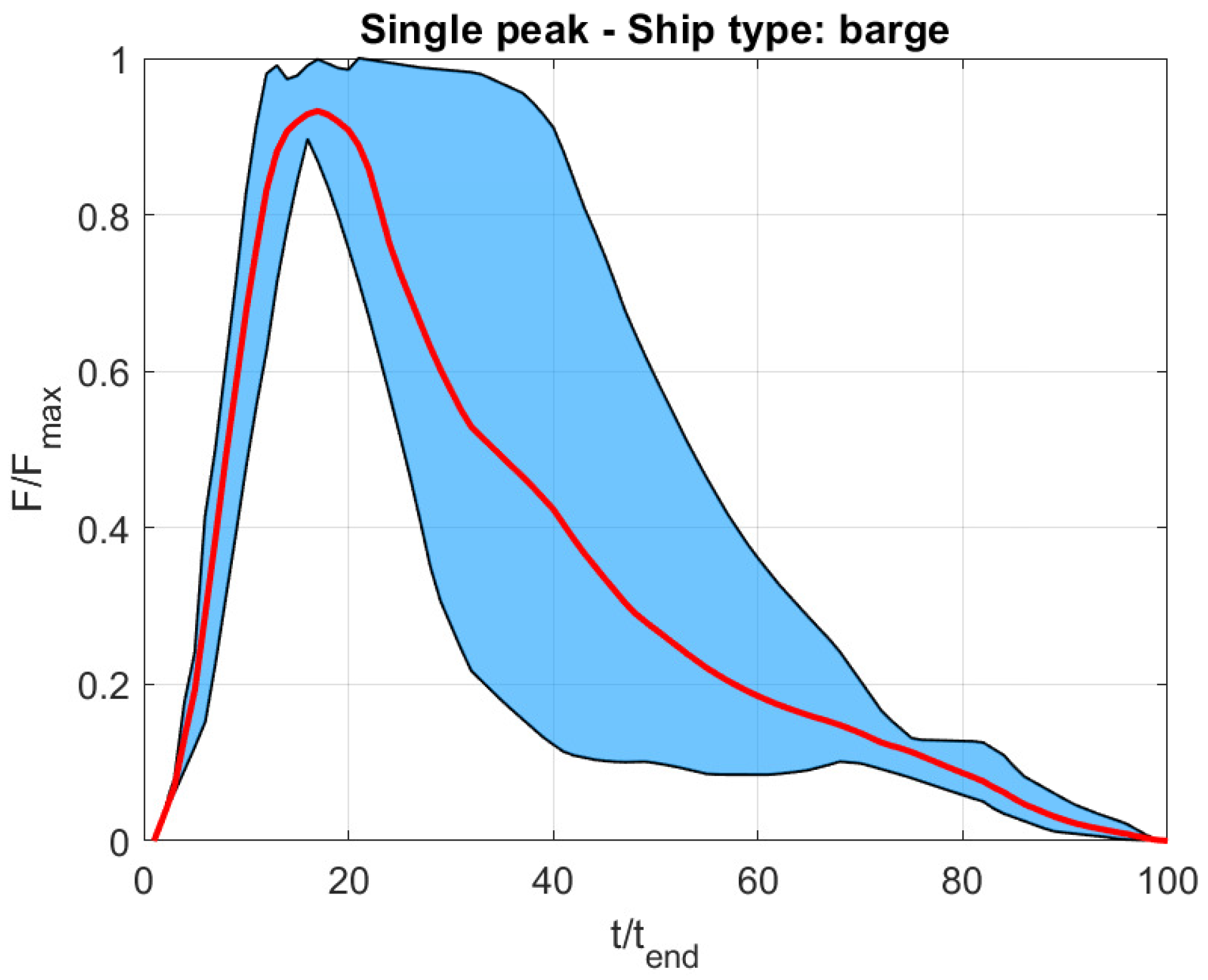
Figure 5.
The time trend of the impact force due to a barge impact. This impact shows single-peak behavior [41,44]. The maximum peak force module is around 5 MN.

Figure 6.
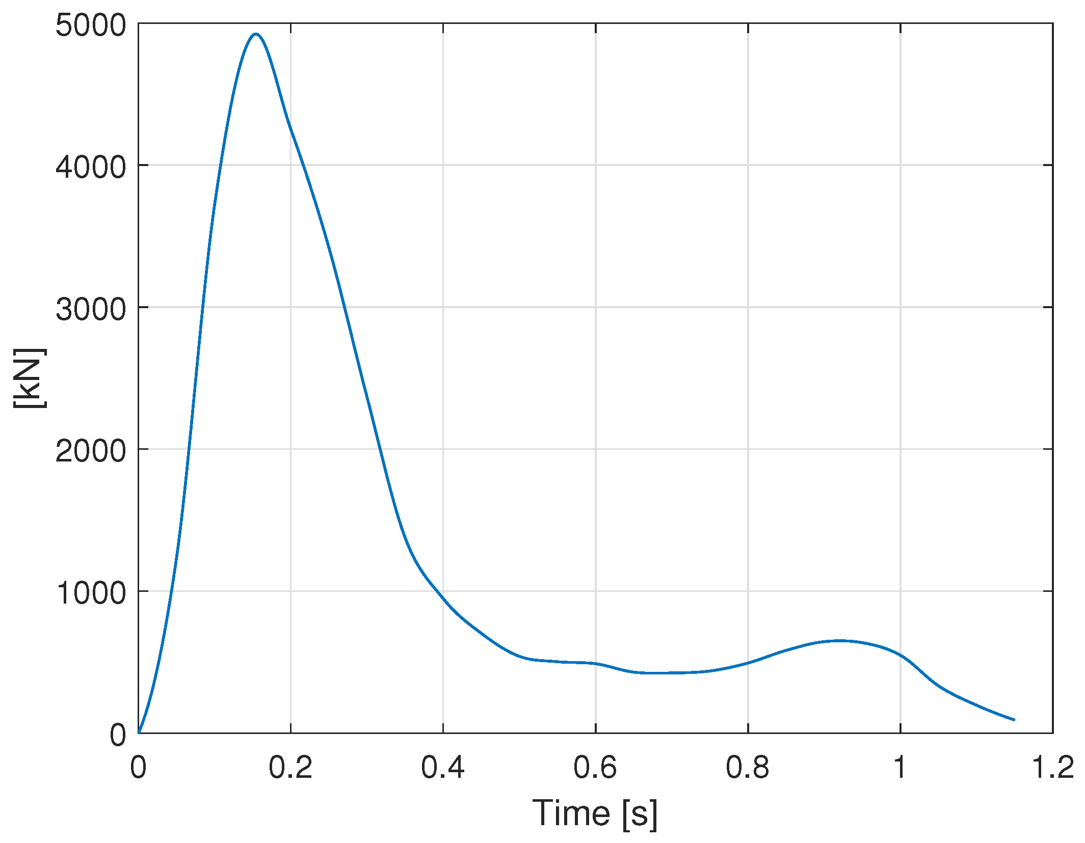
Bulb vessel collision force [39], rescaled, with a peak around 40 MN.
Figure 6.
Bulb vessel collision force [39], rescaled, with a peak around 40 MN.
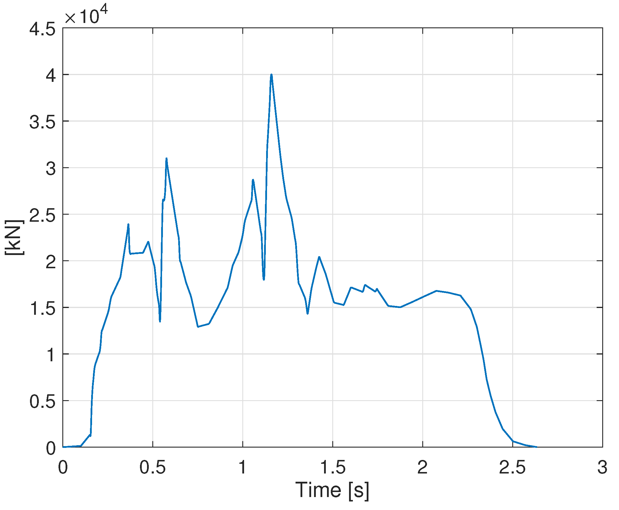
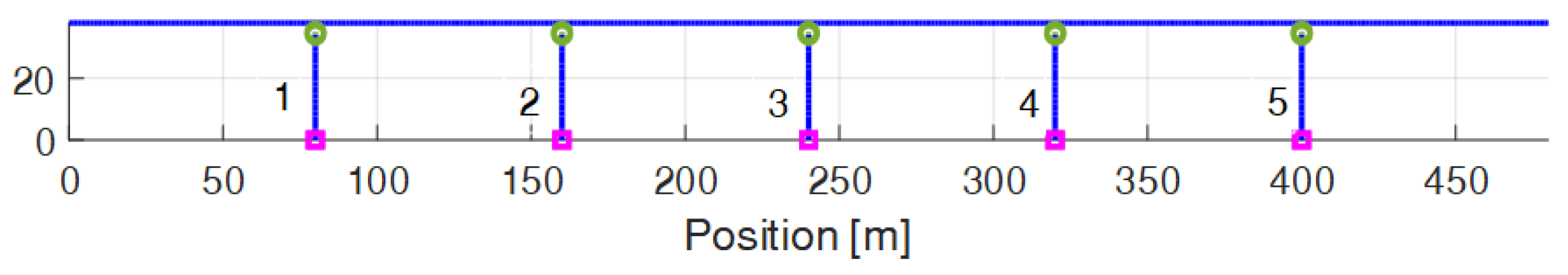
Figure 7.
Lateral view of the unifilar FE model of the considered sea bridge. Impact occurs at pier N. 3.
Figure 7.
Lateral view of the unifilar FE model of the considered sea bridge. Impact occurs at pier N. 3.

Figure 8.
Bridge deck cross-section adopted in the present analysis.

Figure 9.
Bridge main lateral eigenfrequencies and associated mode shapes involved in the dynamical response to a vessel collision.
Figure 9.
Bridge main lateral eigenfrequencies and associated mode shapes involved in the dynamical response to a vessel collision.
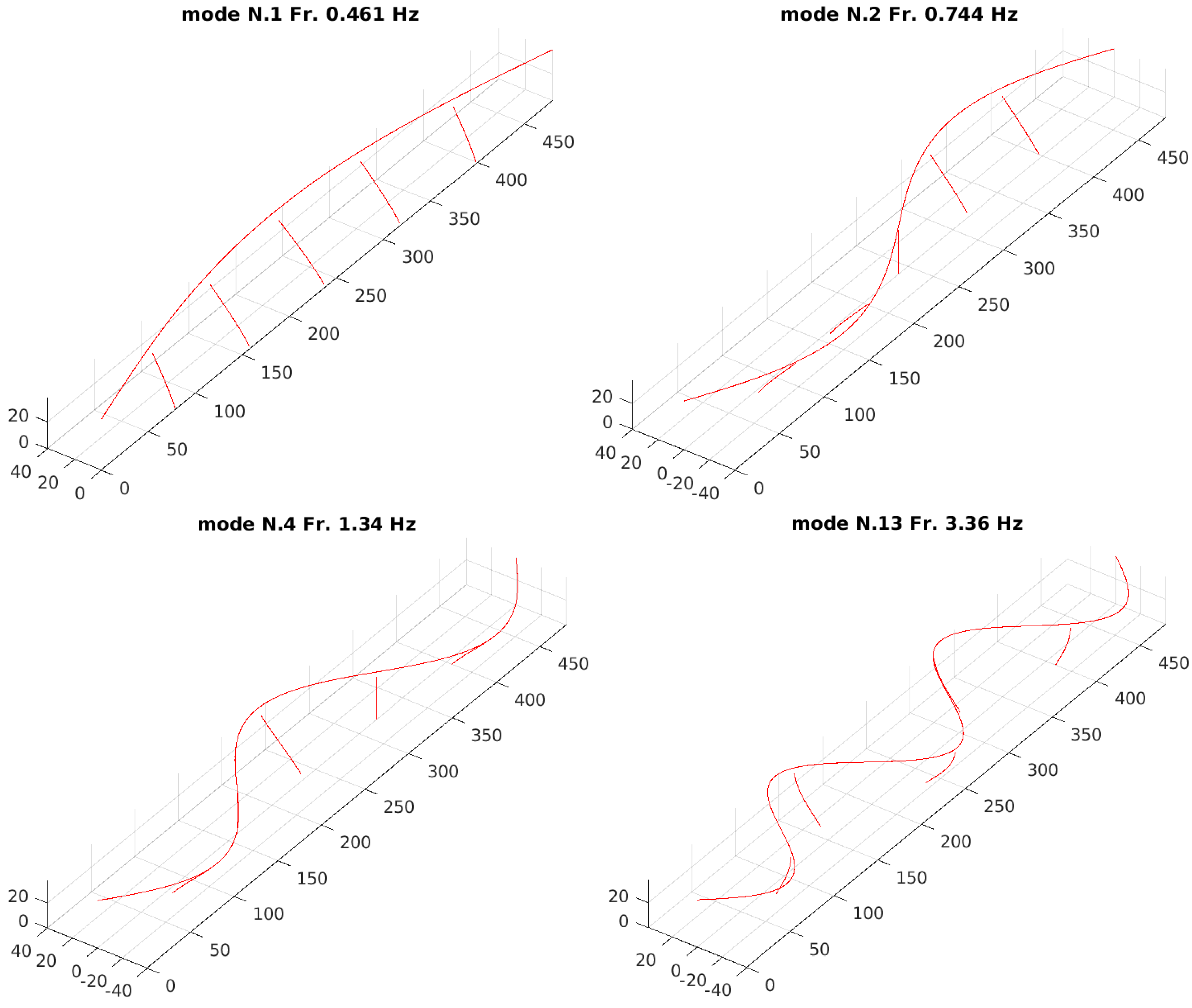
Figure 10.
Track irregularity profile components computed according to [49].
Figure 10.
Track irregularity profile components computed according to [49].
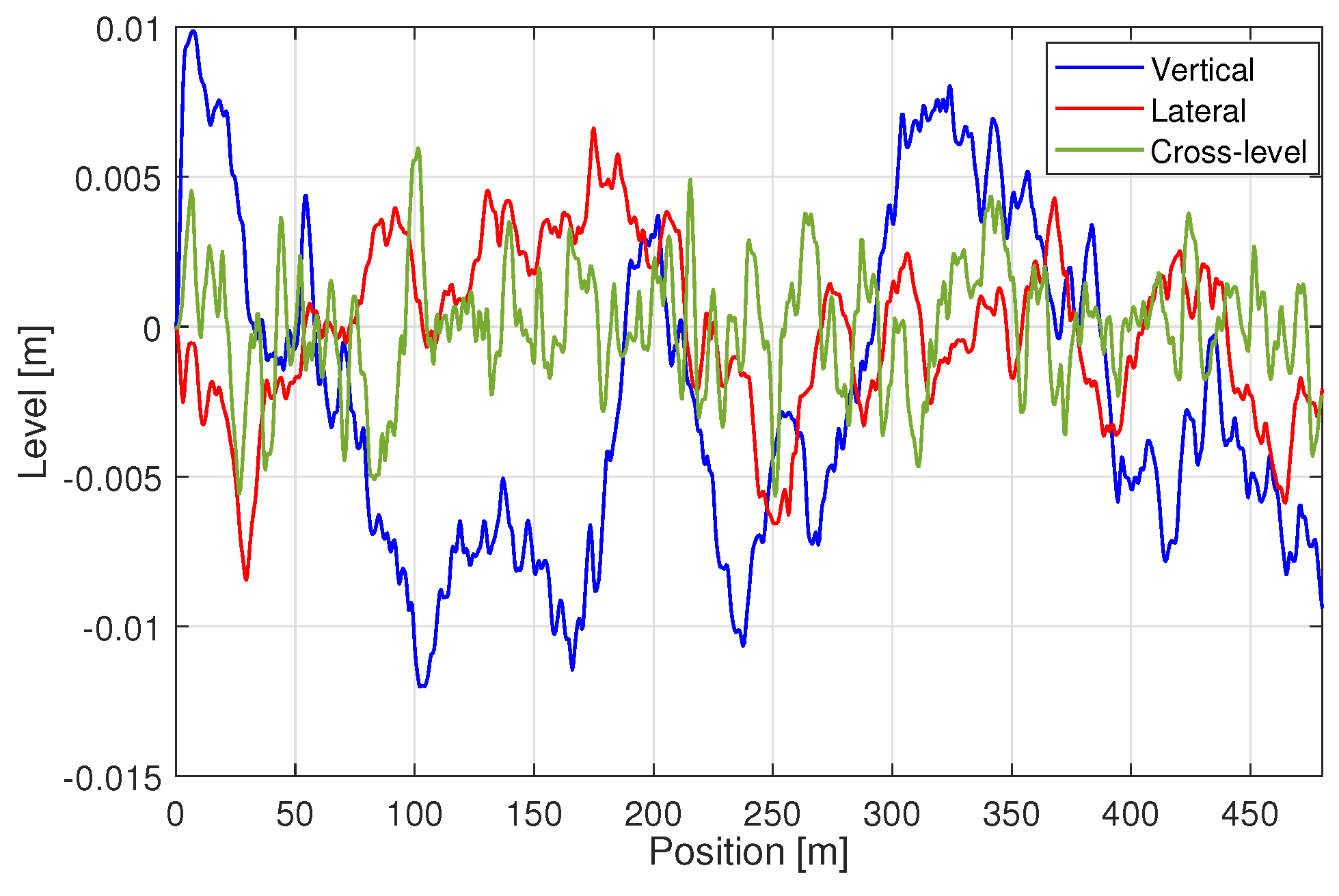
Figure 11.
Thirty-five-degree-of-freedom scheme model of a rail coach. The degrees of freedom and the connections by means of springs and dampers between the rigid bodies are highlighted in the figure.
Figure 11.
Thirty-five-degree-of-freedom scheme model of a rail coach. The degrees of freedom and the connections by means of springs and dampers between the rigid bodies are highlighted in the figure.
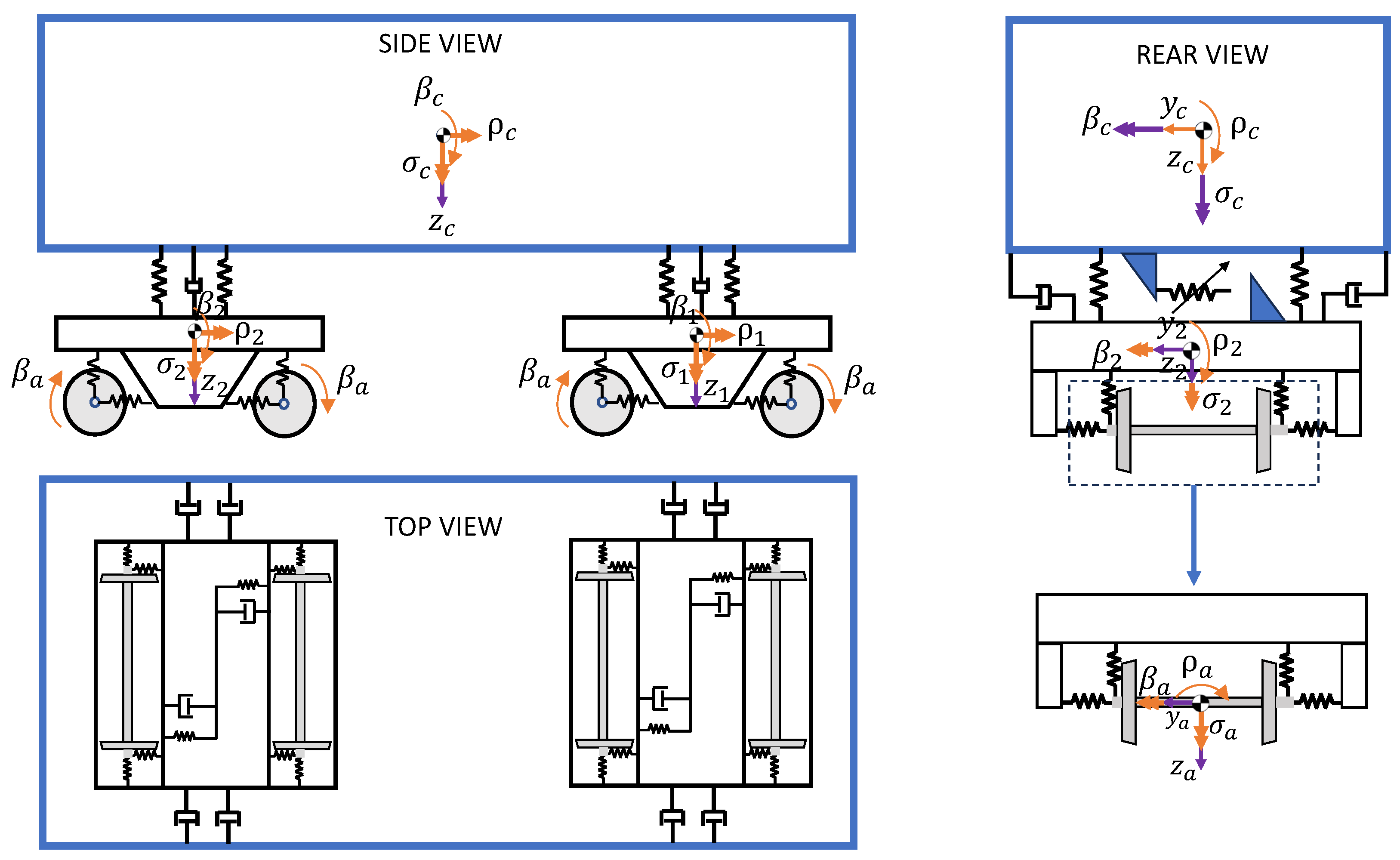
Figure 12.
(a) Wheel–rail vertical and lateral contact force conventions (on left wheel) in the case when only one point of contact is active. (b) Bumpstop force reported as a function of the lateral relative displacement between the car body and the bogie.
Figure 12.
(a) Wheel–rail vertical and lateral contact force conventions (on left wheel) in the case when only one point of contact is active. (b) Bumpstop force reported as a function of the lateral relative displacement between the car body and the bogie.

Figure 13.
Rolling radius variation for left and right wheels as a function of the relative lateral displacement between the wheel and rail. Scenario with new profiles, with an equivalent conicity of 0.05. The right wheel corresponds to negative values of lateral displacement; the left wheel corresponds to positive ones.
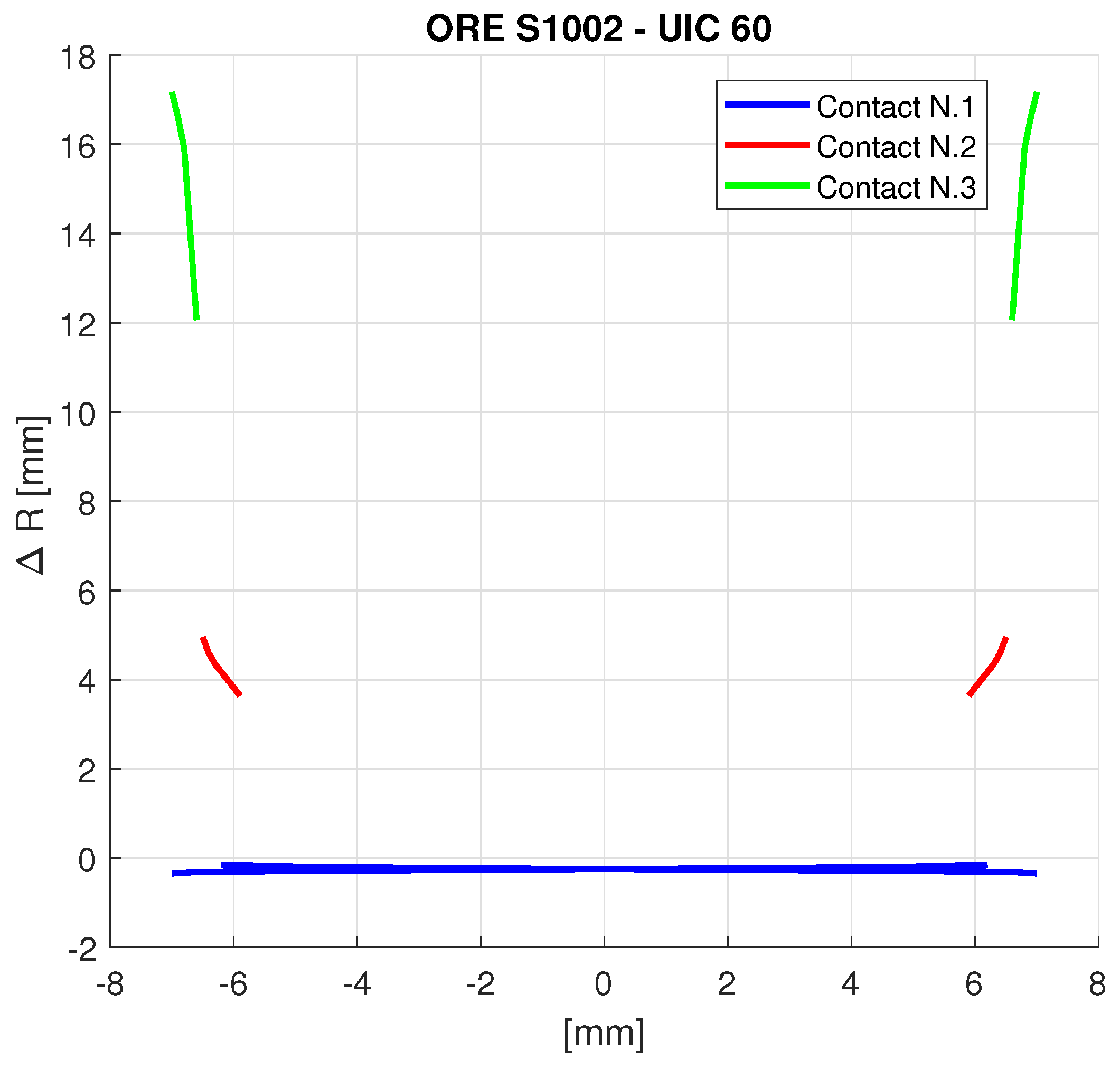
Figure 14.
Location of the possible contact point on the wheel profile (new wheel and rail profiles).
Figure 14.
Location of the possible contact point on the wheel profile (new wheel and rail profiles).

Figure 15.
Rolling radius variation for left and right wheels as a function of the relative lateral displacement between the wheel and rail. Scenario with moderately worn profiles, with an equivalent conicity of 0.15. The right wheel corresponds to negative values of lateral displacement; the left wheel corresponds to positive ones.
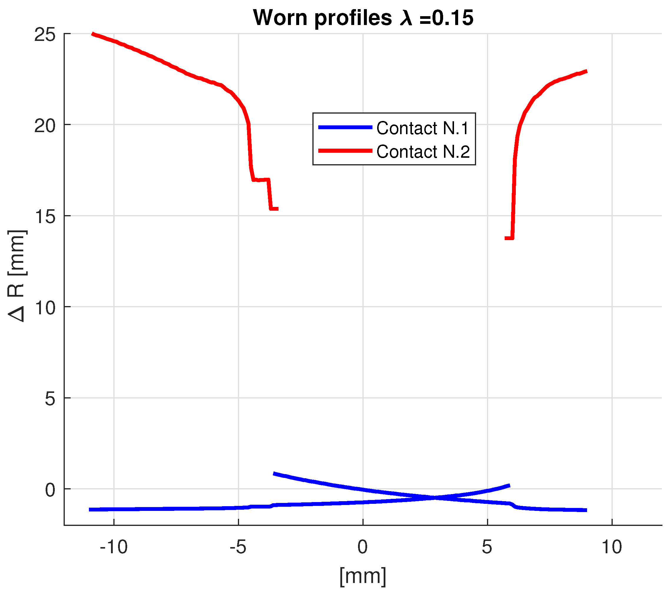
Figure 16.
Numerical time domain integration procedure. The red box identifies the m-th iteration within the i-th time step. The blue box indicates the first approximation of state vectors at the beginning of the i-th time step. refers to the normal contact forces and and stand for the longitudinal and tangential contact forces in the local contact plane for the k-th wheel.

Figure 17.
Displacements and accelerations in the y direction at the impacted pier in the case of a barge impact, scaled to 40 MN, and relative spectra.
Figure 17.
Displacements and accelerations in the y direction at the impacted pier in the case of a barge impact, scaled to 40 MN, and relative spectra.
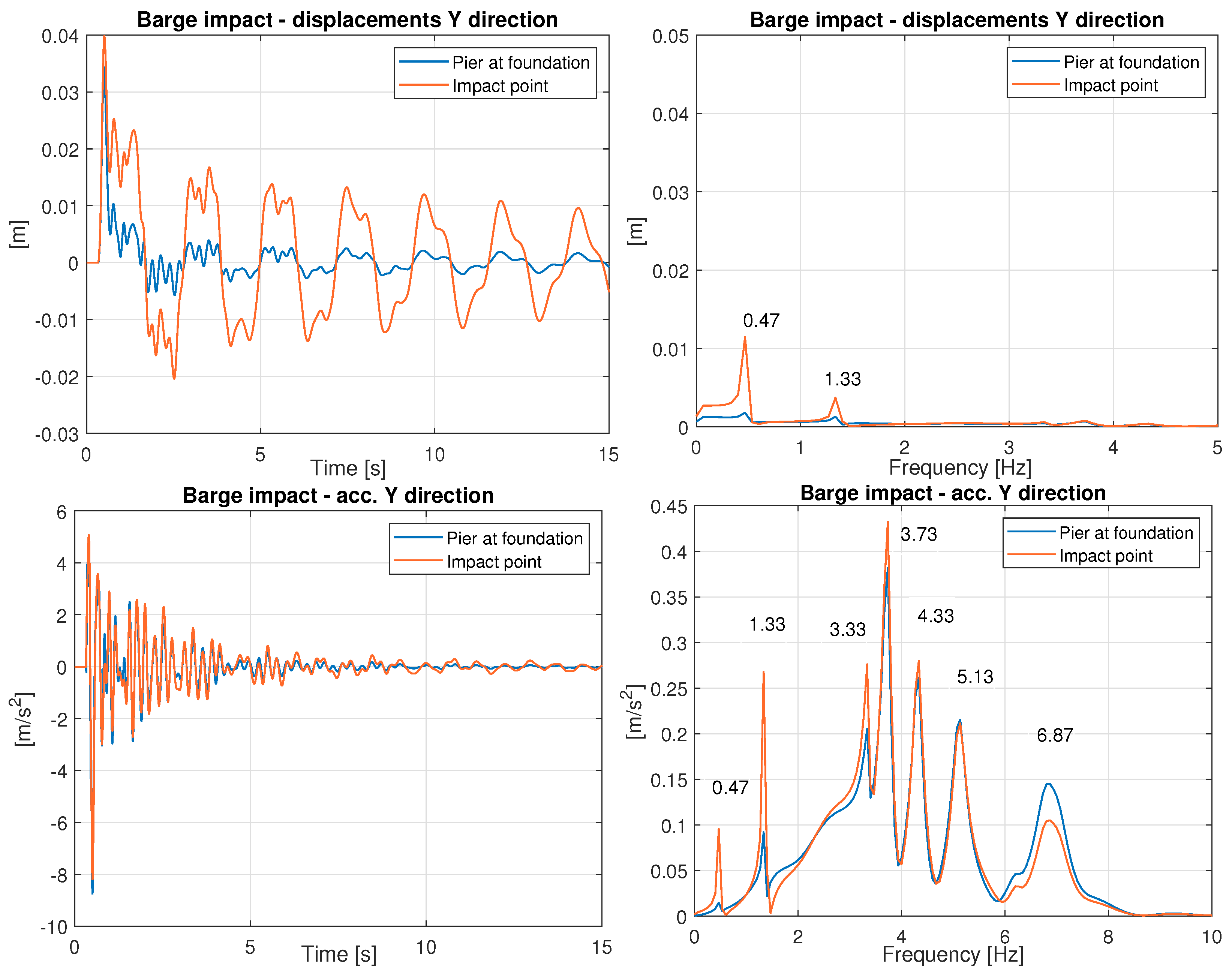
Figure 18.
Displacements and accelerations in the y direction at the deck level in the case of a barge impact, scaled at 40 MN, and relative spectra.
Figure 18.
Displacements and accelerations in the y direction at the deck level in the case of a barge impact, scaled at 40 MN, and relative spectra.
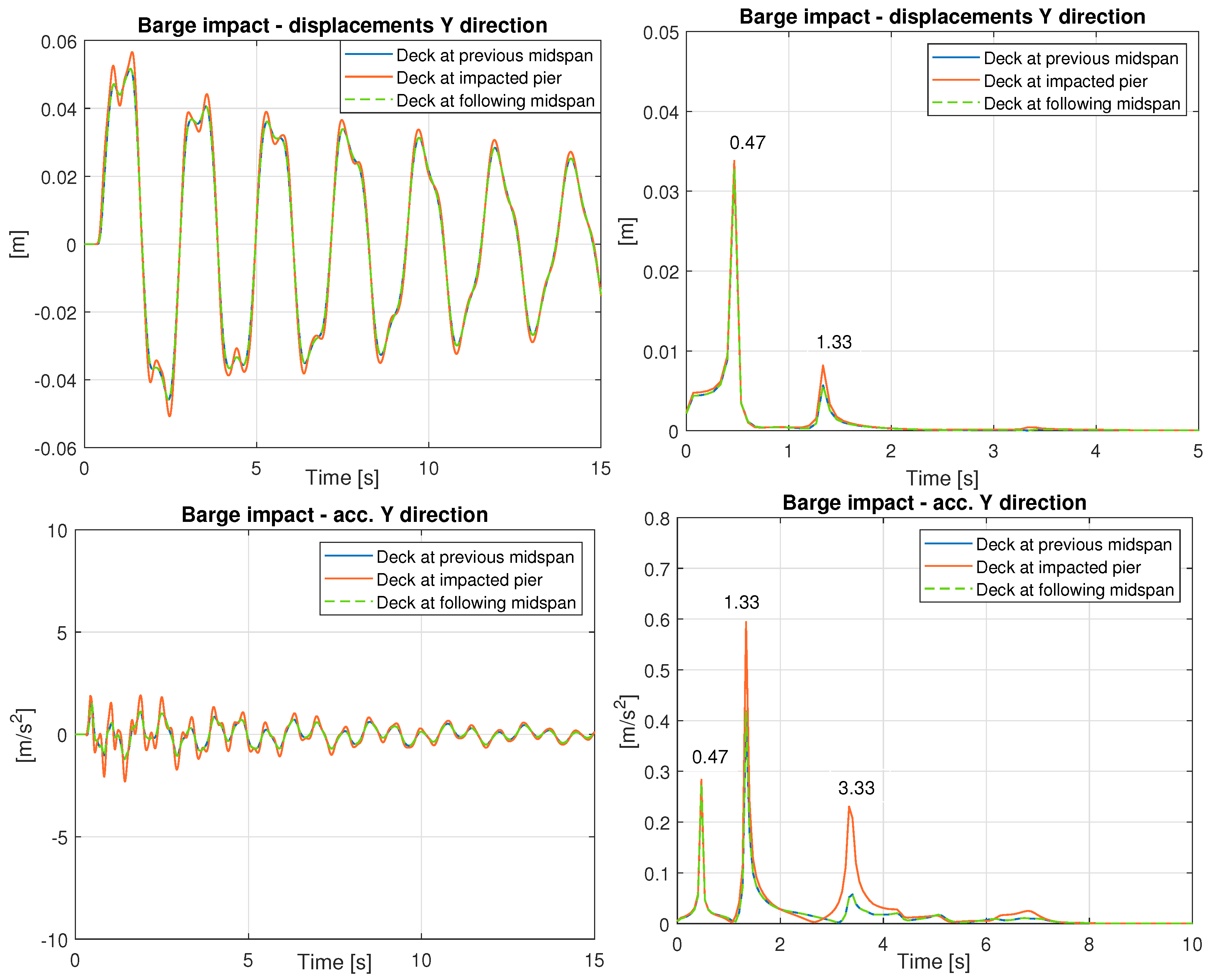
Figure 19.
Displacements and accelerations in the y direction at the affected pier in the case of bulb vessel impact, scaled at 40 MN, and relative spectra.
Figure 19.
Displacements and accelerations in the y direction at the affected pier in the case of bulb vessel impact, scaled at 40 MN, and relative spectra.
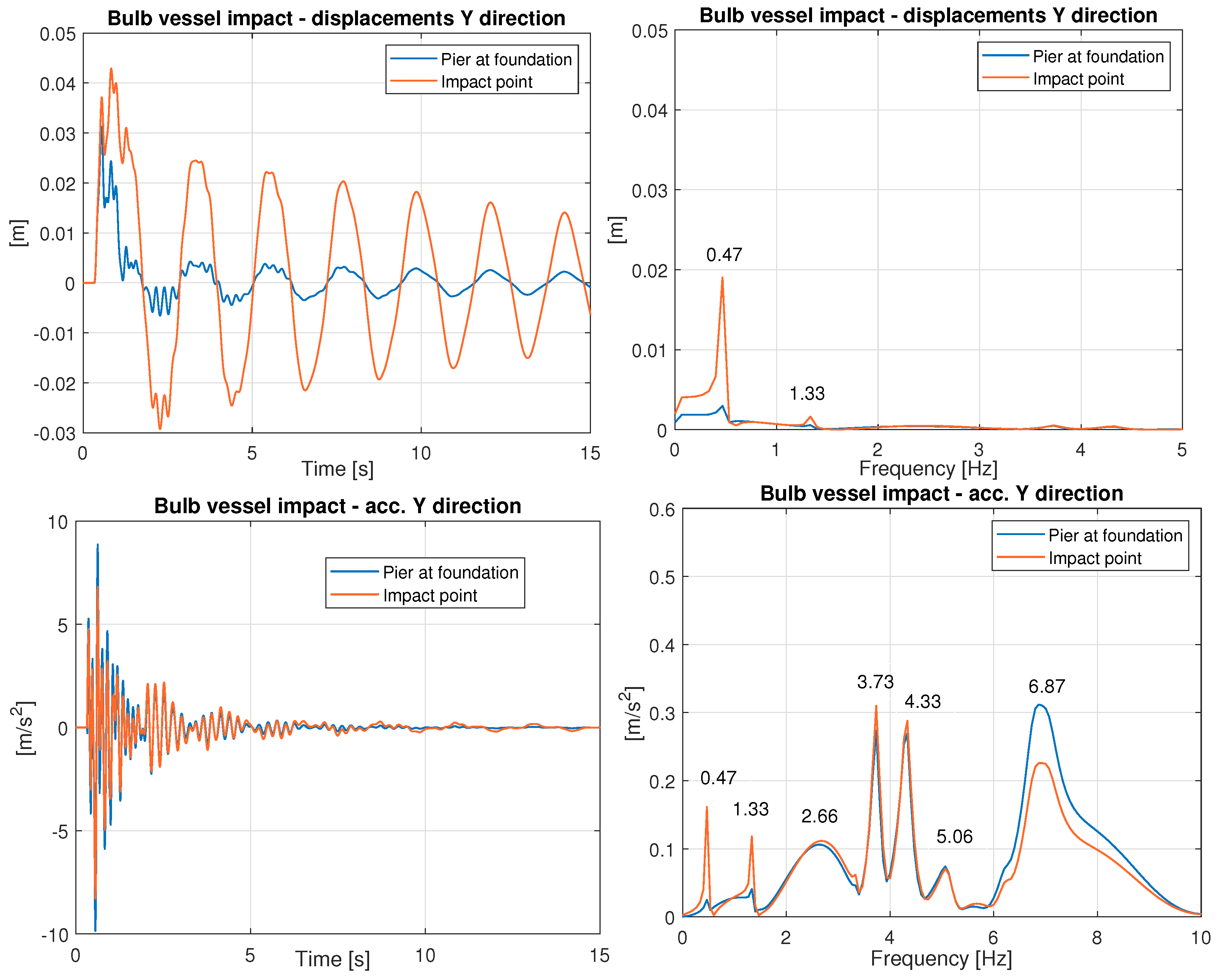
Figure 20.
Displacements and accelerations in the y direction at the deck level in the case of bulb vessel impact, scaled at 40 MN, and relative spectra.
Figure 20.
Displacements and accelerations in the y direction at the deck level in the case of bulb vessel impact, scaled at 40 MN, and relative spectra.

Figure 21.
Schematic representation of the procedure followed to determine the presented coefficients maps.
Figure 21.
Schematic representation of the procedure followed to determine the presented coefficients maps.

Figure 22.
Vertical (Q) and lateral (Y) contact forces for wheel set N. 18 of the adopted train in the case of a barge impact with a 40 MN peak value and a travelling speed of 150 km/h.
Figure 22.
Vertical (Q) and lateral (Y) contact forces for wheel set N. 18 of the adopted train in the case of a barge impact with a 40 MN peak value and a travelling speed of 150 km/h.
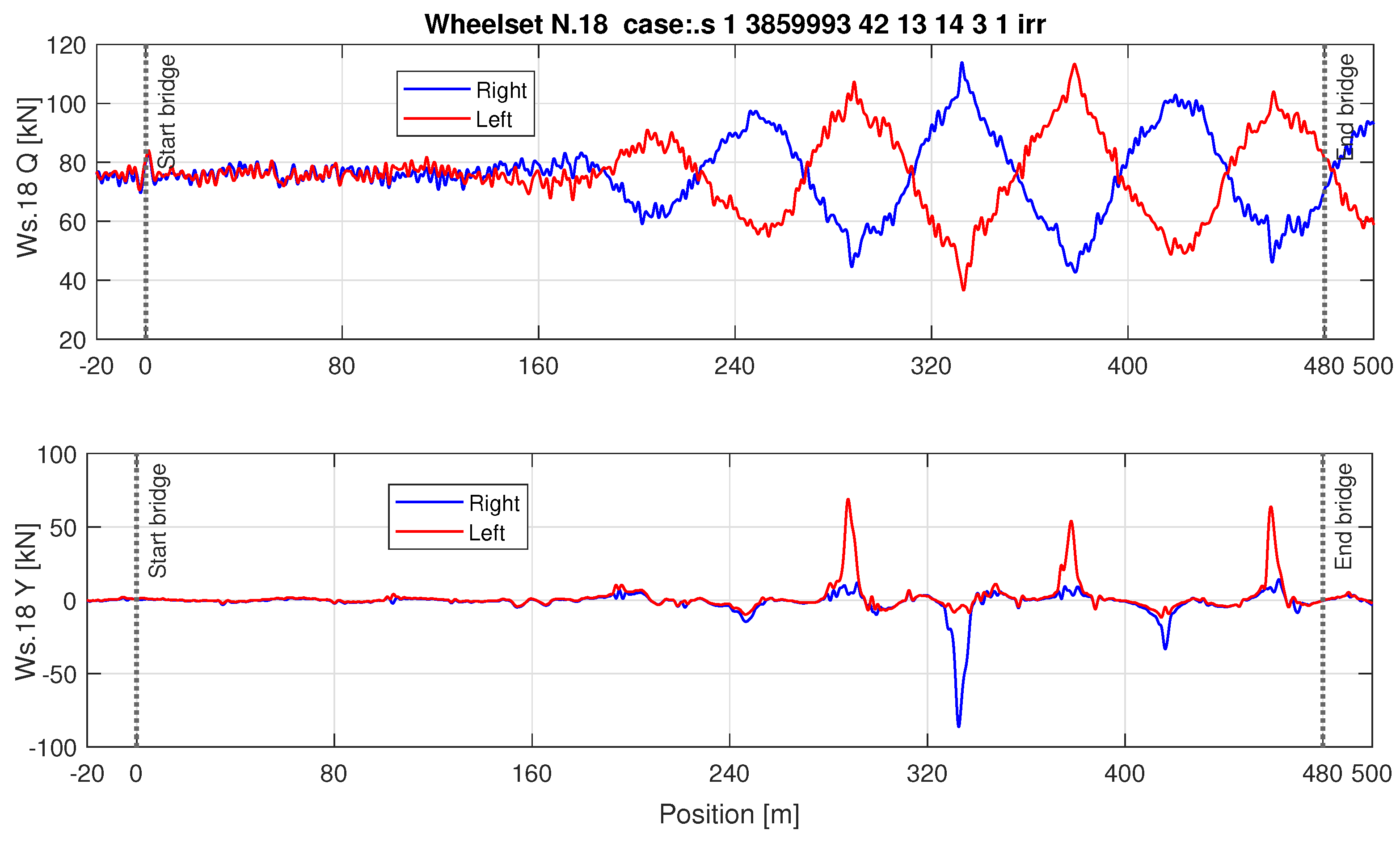
Figure 23.
Derailment and unloading coefficients plotted as a function of the wheel position for wheel set N. 18 in the case of a barge impact with a 40 MN peak value and a travelling speed of 150 km/h.
Figure 23.
Derailment and unloading coefficients plotted as a function of the wheel position for wheel set N. 18 in the case of a barge impact with a 40 MN peak value and a travelling speed of 150 km/h.

Figure 24.
Train running coefficient comparison for each wheel set. The train speed is 150 km/h and the barge impact force is 40 MN.
Figure 24.
Train running coefficient comparison for each wheel set. The train speed is 150 km/h and the barge impact force is 40 MN.

Figure 25.
Distribution of running safety coefficients for the double-deck train in the case of a barge impact. Safety coefficients associated with the new wheel–rail profile are reported on the left (derailment: top and unloading: bottom). The analogous distributions related to the moderately worn profile are illustrated on the right.
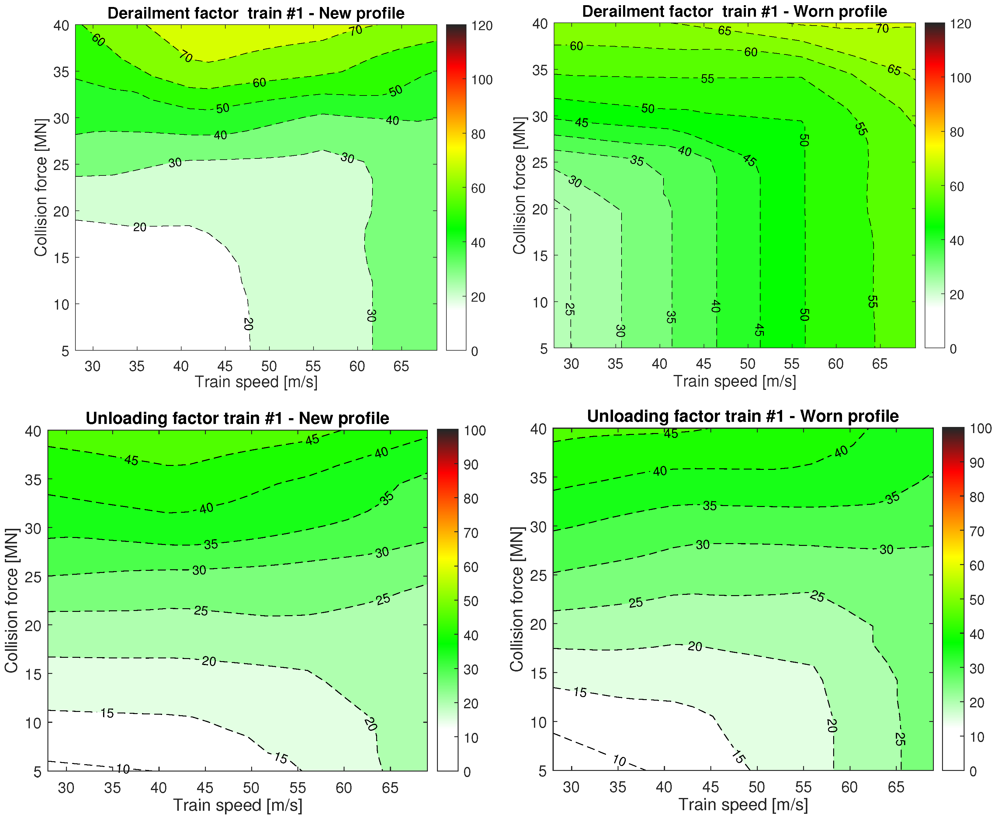
Figure 26.
Distribution of running safety coefficients for the double-deck train in the case of a bulb vessel impact. Safety coefficients associated with the new wheel–rail profile are reported on the left (derailment: top and unloading: bottom). The analogous distributions related to the moderately worn profile are illustrated on the right.

Table 1.
Main geometric and dynamic proprieties of the adopted continuous deck bridge.
| A [m2] | [m4] | I2 [mm4] | I3 [mm4] | E [Gpa] | [kg/m3] | |
|---|---|---|---|---|---|---|
| Piers | 21.9 | 53.0 | 19.0 | 83.0 | 35.2 | 2460.0 |
| Deck | 25.8 | 173.0 | 879.0 | 69.0 | 35.2 | 2760.0 |
| Rayleigh Damping Coefficients | ||||||
| Piers | 0.1 | 0.001 | ||||
| Deck | 0.1 | 0.001 | ||||
| Span [m] | Width [m] | Height [m] | Mass per Meter [kg/m] | |||
| Deck | 6× | 80.0 | 25.0 | 4.5 | 71,208.0 | |
| Modes | L1 | L2 | L3 | L4 | ||
| Freq. [Hz] | 0.47 | 0.74 | 1.33 | 3.36 | ||
Table 2.
Parameters of bridge foundations and bearings modeled as linear springs and dampers.
| Foundation | Deck Bearings | |
|---|---|---|
| [N/m] | 9.50 | 0.00 |
| [N/m] | 9.47 | 4.00 |
| [N/m] | 3.92 | 4.00 |
| [N·m/rad] | 8.47 | 3.92 |
| [N·m/rad] | 1.04 | 0.00 |
| [N·m/rad] | 9.95 | 0.00 |
| [N·s/m] | 9.50 | 0.00 |
| [N·s/m] | 1.89 | 4.00 |
| [N·s/m] | 3.92 | 4.00 |
| [N·m·s/rad] | 4.24 | 3.92 |
| [N·m·s/rad] | 5.20 | 0.00 |
| [N·m·s/rad] | 4.98 | 0.00 |
Table 3.
Train first lateral eigenfrequencies. H stands for head coach, M for motorized coach, and T for trailer coach.
Table 3.
Train first lateral eigenfrequencies. H stands for head coach, M for motorized coach, and T for trailer coach.
| Double-Deck Train | |||
|---|---|---|---|
| Configuration | H–T–T–M–M–T–T–H | ||
| Lat. [Hz] | Yaw [Hz] | Vert. [Hz] | |
| M, H | 0.46 | 0.76 | 0.9 |
| T | 0.45 | 0.83 | 0.84 |
Disclaimer/Publisher’s Note: The statements, opinions and data contained in all publications are solely those of the individual author(s) and contributor(s) and not of MDPI and/or the editor(s). MDPI and/or the editor(s) disclaim responsibility for any injury to people or property resulting from any ideas, methods, instructions or products referred to in the content. |
© 2024 by the authors. Licensee MDPI, Basel, Switzerland. This article is an open access article distributed under the terms and conditions of the Creative Commons Attribution (CC BY) license (https://creativecommons.org/licenses/by/4.0/).
Share and Cite
MDPI and ACS Style
Bernardini, L.; Collina, A.; Soldavini, G. Railway Bridge Runability Safety Analysis in a Vessel Collision Event. Vibration 2024, 7, 326-350. https://doi.org/10.3390/vibration7020016
AMA Style
Bernardini L, Collina A, Soldavini G. Railway Bridge Runability Safety Analysis in a Vessel Collision Event. Vibration. 2024; 7(2):326-350. https://doi.org/10.3390/vibration7020016
Chicago/Turabian StyleBernardini, Lorenzo, Andrea Collina, and Gianluca Soldavini. 2024. "Railway Bridge Runability Safety Analysis in a Vessel Collision Event" Vibration 7, no. 2: 326-350. https://doi.org/10.3390/vibration7020016