Relativistic Mean-Field Models with Different Parametrizations of Density Dependent Couplings


1
Institut für Kernphysik, Technische Universität Darmstadt, Schlossgartenstraße 9, 64289 Darmstadt, Germany
2
GSI Helmholtzzentrum für Schwerionenforschung GmbH, Planckstraße 1, 64291 Darmstadt, Germany
Particles 2018, 1(1), 3-22; https://doi.org/10.3390/particles1010002
Submission received: 16 January 2018
/
Revised: 29 January 2018
/
Accepted: 30 January 2018
/
Published: 2 February 2018
(This article belongs to the Special Issue Selected Papers from “The Modern Physics of Compact Stars and Relativistic Gravity 2017”)
Abstract
:Relativistic mean-field models are successfully used for the description of finite nuclei and nuclear matter. Approaches with density-dependent meson-nucleon couplings assume specific functional forms and a dependence on vector densities in most cases. In this work, parametrizations with a larger sample of functions and dependencies on vector and scalar densities are investigated. They are obtained from fitting properties of finite nuclei. The quality of the description of nuclei and the obtained equations of state of symmetric nuclear matter and neutron matter below saturation are very similar. However, characteristic nuclear matter parameters, the equations of state and the symmetry energy at suprasaturation densities show some correlations with the choice of the density dependence and functional form of the couplings. Conditions are identified that can lead to problems for some of the parametrizations.

1. Introduction
A realistic description of dense matter is essential for the physics of compact stars and the simulation of core-collapse supernovae and neutron-star mergers; see, e.g., [1] for details. Depending on the thermodynamic conditions, a variety of particle species has to be considered in the construction of microscopic models; in particular, nucleons and electrons are indispensable in astrophysical applications. The thermodynamic properties of such matter are encoded in the equation of state (EoS). In general, the EoS depends on several variables, e.g., the baryon number density , the temperature T and the electron fraction . They cover several orders of magnitude in the application, and the properties of matter change dramatically within the corresponding ranges. The main theoretical challenge is the description of the hadronic component, i.e., the subsystem composed of nucleons (and possibly other baryons such as hyperons at very high densities) that interact strongly. The leptonic component can be well treated in a simple Fermi gas model in most cases.
At baryon densities below the nuclear saturation density fm and temperatures not exceeding approximately K or MeV, matter is not homogeneous, and structures develop due to the competition of the short-range strong interaction, the long-range Coulomb interaction and the entropy. For instance, neutron-rich nuclear clusters can form that arrange on a lattice in the crust of neutron stars. At densities around and above , e.g., in the core of compact stars, or at high temperatures, matter is expected to be homogeneous. The description of such uniform hadronic matter is the subject of this work.
There are many microscopic theoretical approaches to construct EoSs of strongly-interacting matter. One class of models is based on realistic interactions, which are fitted to nucleon-nucleon scattering data and properties of light nuclei, in combination with sophisticated techniques to solve the many-body problem. In contrast, in a second class of models, phenomenological approaches proceed more heuristically employing effective interactions with a number of parameters that can be determined from experimental data of different origin. These approaches are often derived from self-consistent mean-field (MF) models [2]. They can be expressed as energy density functionals (EDF), which, in principle, are able to capture the essential features of the system. Amongst them, EDFs based on non-relativistic Hartree–Fock calculations with Skyrme or Gogny potentials are most familiar [3,4]. Relativistic or covariant EDFs can be constructed from relativistic mean-field (RMF) models that describe the strong interaction by an exchange of mesons, which are are usually assumed to couple minimally to nucleons.
For a quantitative description of nuclei and nuclear matter, medium effects of the effective interaction have to be included. This can be achieved in different ways. In a large number of RMF models [5], nonlinear (NL) self-interactions of the mesons are incorporated in the Lagrangian density that defines the model. Alternatively, the meson-nucleon couplings in can contain an explicit dependence on the nucleon field operators that is mapped to a density dependence of the couplings in the derived EDF. The choice of the functional form of this dependence facilitates a very flexible variety of models. The parameters of the density dependence are customarily determined by applying the EDF to the description of finite nuclei and by fitting to a selected set of their properties.
A particular property of RMF models is the occurrence of two different particle number densities: vector densities and scalar densities. Their interplay is essential to describe the saturation of nuclear matter in the model. RMF models with density-dependent (DD) couplings were first applied to the description of finite nuclei by Fuchs and Lenske [6,7] considering dependencies on vector and scalar densities. The couplings were obtained from microscopic Dirac–Brueckner–Hartree–Fock calculations of nuclear matter. The first self-consistent RMF model with density-dependent couplings that were fitted to properties of finite nuclei used the so-called vector density in the couplings and specific forms for the functional dependence [8]. Many subsequent models and parametrizations followed this approach, sometimes introducing different functions; see, e.g., [9,10,11,12,13,14,15]. A dependence on other densities, in particular the scalar density, in the description of nuclei was not really explored. The aim of this work is a comparison of RMF models and the corresponding nuclear matter EoSs with DD couplings of different functional form and dependencies on vector and scalar densities that were fitted to the same set of nuclear observables.
The formalism of RMF models with DD couplings is presented in Section 2 with applications to homogeneous nuclear matter and finite nuclei. The parametrization of the meson-nucleon couplings is introduced in Section 3. The determination of the parameters and the form of the couplings is discussed in Section 4. Properties of nuclear matter and the EoS are summarized in Section 5 including the characteristic nuclear matter parameters and the density dependence of the symmetry energy. In Section 6, constraints on the possible density dependence of the couplings are considered. Conclusions are given in Section 7, and the actual values of the different parameter sets are collected in Appendix A. Natural units with are used throughout this paper.
2. RMF Model with Density-Dependent Couplings
The theoretical description of nuclei and nuclear matter in the present RMF approach proceeds in the usual way as presented, e.g., in [8]. The strong interaction is described by an exchange of isoscalar and mesons and isovector and mesons. They carry the same quantum numbers as the corresponding experimentally-known mesons, but they are not necessarily the same. However, in this way, it is possible to capture the main features of the effective in-medium nuclear interaction. The mesons couple minimally to the nucleons that are represented by four-spinor operators forming an isospin doublet. The coupling with a meson , , or is denoted by , a functional that can depend on suitable combinations of and , where is a Dirac matrix. In the present work, a dependence on the vector density:
with the nucleon current:
or the scalar density:
is considered. Despite the name, the vector density (1) is a Lorentz scalar, as well as the scalar density (3). This guarantees the Lorentz covariance of the approach. In addition to the meson fields, a coupling to the electromagnetic field, represented by the vector field , with constant coupling strength is taken into account.
2.1. Lagrangian Density and Energy Density Functional
The starting point of the formalism is the Lagrangian density:
with three contributions. The first:
contains the covariant derivative:
where () are isospin matrices in analogy with the Pauli matrices , but acting in isospin space. The effective mass operator has the form:
with the nucleon masses in vacuum. The and terms carry an arrow since they have three components in isospin space. In contrast, the and fields are isoscalar quantities. The meson term in Equation (4) has the standard form:
with meson masses and field tensors: and for the vector mesons. The last contribution in Equation (4) is the Lagrangian density of the electromagnetic/photon field:
with . It is only relevant for finite nuclei, and not for homogeneous nuclear matter.
The field equations for all degrees of freedom are derived with the help of the Euler–Lagrange equations in the standard mean-field and no-sea approximation. Mesons and photons are treated as classical fields. This leads to the Dirac equation for the nucleons, Klein–Gordon and Proca equations for scalar and vector mesons, respectively, and the Maxwell equation for the electromagnetic field. Using symmetries, e.g., by a restriction to a stationary system and choosing a particular frame of reference, i.e., breaking Lorentz covariance, the equations simplify further.
In the MF approximation of the present approach, the coupling functionals become simple functions of the total vector density with:
and the total scalar density with:
where denotes the occupation factor of the single-particle state k of nucleon i. The nucleon wave functions are solutions of the time-independent Dirac equation:
with scalar and vector potentials and , respectively. They are given by:
with factors and that reflect the different coupling of neutrons and protons to the fields. Due to symmetries, only a single component of the Lorentz vector and isospin vector fields remains; hence, the notation is simplified to , , and without an additional index for the isospin in the following.
The potentials (13) and (14) contain the rearrangement terms:
that arise due to the density dependence of the couplings . These terms are identical for all particles since the couplings depend only on the sum of the scalar and vector densities, and in the present work. The source densities in Equations (15) and (16) are found from:
for scalar mesons and:
for vector mesons by simple summations over the nucleons.
The energy density:
is obtained from the energy-momentum tensor where the brackets denote the summation over all occupied states in the system. The contribution of the nucleons has the form:
and the contribution of the fields reads as:
The energy density (19) is a functional of the nucleons (, ), the fields (, , , , ) and their derivatives (, , , , ). Similar to the Lagrangian density (4), it can be used to derive the field equations:
with the source density:
in the Poisson Equation (26) for the electromagnetic potential .
2.2. Homogeneous Nuclear Matter
In this case, the theoretical description simplifies further. The solutions of the Dirac Equation (12) are plane waves with momentum p and energy:
for particles () and antiparticles (), which have to be included when finite temperatures are considered. The meson fields and densities are constants in space. There is no contribution from the electromagnetic field because the source density is constant, and, thus . The energy density can be written as:
with the quantities:
and:
and the kinetic contribution:
in the continuum limit containing the degeneracy factor for the spin nucleons. Rearrangement contributions in the energy density (29) appear only if the couplings depend on the scalar density , i.e., . The Fermi–Dirac distribution functions:
in Equation (32) depend on the energy , the chemical potential and the temperature T. These functions also appear in the vector and scalar densities:
with the Dirac effective mass:
Additional thermodynamic quantities are easily calculated. The entropy density assumes the standard form:
The pressure:
can be obtained from the energy-momentum tensor. The result is identical to that of the thermodynamic definition:
as a derivative of the energy density with respect to the total baryon density for constant temperature T and isospin asymmetry . The rearrangement terms are essential for the thermodynamic consistency.
For vanishing temperature, as considered in most cases of this work, there are no antiparticle contributions, and analytical results are available for the vector density:
with the Fermi momentum and the scalar density:
with the effective chemical potential:
The expression (32) reduces to:
and the pressure can be written as:
with:
and the kinetic contribution:
Obviously, the entropy density (37) vanishes for .
2.3. Finite Nuclei
The energy of a nucleus with N neutrons and Z protons in the RMF calculation is found as:
with single-particle energies and corresponding occupation numbers of the single-particle states k of nucleon i. They satisfy the normalization conditions:
Using the field equations, the contribution of the meson and electromagnetic fields in Equation (47) can be written as:
with factors:
that contain derivatives of the coupling functions.
In the present work, only spherical nuclei are considered. In this case, the single-particle wave functions can be written as:
with real radial wave functions and and spin-spherical harmonics . They depend on the quantum number , , ..., which determines the total angular momentum and the orbital angular momentum of the state, and the projection , i.e., there is a -fold degeneracy of the level with energy . Assuming equal occupation of the sub-states, the vector and scalar single-particle densities are given by:
with the normalization:
This assures the sphericity of the source densities and potentials.
For a comparison with experimental data, the MF energy (47) and quantities related to the density distributions have to be corrected. The Coulomb potential in the calculation of the single-particle wave functions of nucleus with Z protons is multiplied with a factor to have the correct asymptotic dependence of the field when a proton is separated from the nucleus. This is necessary because in the MF approximation, exchange terms are missing that would correct this error. A similar correction for the meson fields is not applied because they are of short range.
Since the nuclear wave functions are fixed in the calculation to the origin of a spherical coordinate system, the translation symmetry is broken and a center-of-mass correction has to be applied. The energy (47) contains a ‘localization’ contribution that has to be subtracted. Here, in a non-relativistic approximation, the expectation value:
for the nucleus with nucleons with the total momentum is used. In the same spirit, a correction for the density distributions is implemented. In a first step, the point particle distributions are converted to form factors by Fourier transformations. These are multiplied by the correction factor:
with for momentum q and form factors for the charge distributions of neutrons and protons if required. An inverse Fourier transformation yields the corrected distributions that can be used, e.g., in the calculation of root-mean-square radii. Further corrections, e.g., from pairing or particle-vibration couplings, are not taken into account. They can be considered in future extensions of this work.
3. Parametrization of Couplings
The density-dependent couplings for , , , are the central quantities that determine the quality of the relativistic density functional. They are usually written in the form:
with a constant coupling at a reference density and an arbitrary function that depends on the ratio . The density n can be any density that is formed as a Lorentz scalar from the single-particle wave functions and . The most frequent choice is a dependence on the total vector density that reduces to the sum:
with the total neutron and proton vector densities and , respectively, in a system at rest without nucleon currents. In this work, also a dependence on the scalar density:
is explored that has been suggested already when the RMF model with DD couplings was developed, but the quality of describing nuclear matter or finite nuclei was not examined in detail. For a dependence on , the reference density is chosen as the vector density at saturation , whereas the scalar density at saturation is used for a dependence on .
The most widely-used form for is a rational function:
with four parameters , , and . It was introduced in [8] for the couplings of the and meson because such a function could describe very well effective density-dependent couplings that were extracted from self-energies in Dirac–Brueckner calculations of nuclear matter. For the meson, a simple exponential form:
with only one parameter was used in [8]. Subsequently, also other functions were devised. For instance, a generalization of (60) as:
was used in [12] with also four parameters as in Equation (59). A specific feature of the functions (59) and (60) is that they are well-behaved for approaching a constant or zero, respectively. In contrast, the function (61) diverges for . A still different form was introduced in [13] as:
for all mesons with an additional modification for the meson close to the saturation density. The latter two functional forms will not be used in this work.
In order to reduce the number of free parameters in the rational function (59), several conditions are demanded. First of all, it is required that . This fixes the first parameter in (59) as:
and leads to the fact that the prefactor in Equation (56) can really be identified with the value of the coupling at the reference density . The function (60) automatically conforms to this condition. In [8], a second condition was introduced, requiring that the curvature of the function (59) vanishes at , i.e., the derivative is . This is met if the relation holds. In [8], only the solution with was explored, whereas the second possibility will be investigated here, as well. Instead of introducing a condition for the second derivative of the function at , the first derivative at this point can be set to a specific value as a third option. In this work, the choice is examined, corresponding to . With these conditions on the function at and , the number of independent parameters reduces to two, one more than for the exponential function (60).
Several combinations for the choice of the density in the argument x, the functional form of the function and the conditions on are explored in this work. In order to summarize these options in a concise form, a three-letter abbreviation is introduced for the identification. There are three cases for the first letter:
- ‘V’: dependence of all functions on ,
- ‘S’: dependence of all functions on ,
- ‘M’: dependence of and on and and on .
The second letter indicates the condition on the rational function for the couplings of the and mesons:
- ‘P’: , (positive),
- ‘Z’: , (zero),
- ‘N’: , (negative).
The last letter denotes the coupling of the and mesons:
The last condition of the case ‘R’ is motivated by the density dependence of the exponential function close to and reduces the number of independent parameters by one. In total, there are different combinations of functions tested in this work.
4. Determination of Parameters and Couplings
As every phenomenological model, the RMF approach with DD couplings depends on a number of parameters that need to be determined by a comparison of model predictions to experimental data. The resulting values will depend on the chosen observables and the method of the fitting procedure. In the present model, the parameters comprise the masses of the nucleons (, p) and mesons (, , , ), the couplings of the mesons at the reference density, the parameters of the functions and the electromagnetic coupling constant . Not all of them are assumed to be free parameters that can be varied more-or-less arbitrarily.
The masses of the nucleons and of the mesons, except the meson, are taken as preassigned with MeV, MeV, MeV, MeV and MeV. The coupling is given by the experimental value. This leaves one mass (), four couplings at the reference density () and six parameters of the functions (two for two isoscalar and one for two isovector mesons) as free parameters of the model. Thus, in total, there are at most 11 parameters that have to be determined. In this work, a contribution of the meson will not be considered, hence there are free parameters left, which are denoted by in the following. In the actual fitting procedure, the six parameters for the couplings of the isoscalar mesons are not used directly because they are highly correlated. Instead, they are replaced by the characteristic values of nuclear matter parameters, i.e., the saturation density, the binding energy per nucleon and the effective mass at saturation, the incompressibility and two parameters related to the ratios of the coupling function and . The conversion between these parameter sets is analytic and easily implemented.
The actual set of parameter values is obtained from a least-squares fit by minimizing the function:
in the multidimensional parameter space. The function is a summation of contributions from observables, comparing experimental data with the parameter-dependent model values and weighted by the inverse of an assigned uncertainty . The latter are not the experimental errors, but values that reflect the hopefully achievable uncertainties of the model. The relative size for different observables also determines their relative importance in the fit. The selection of the observables and their uncertainties directly influences the results. There are different approaches to set up the fitting protocol. In this work, only observables of finite nuclei are considered, but no data that are derived more indirectly like nuclear matter parameters. This choice is motivated by the perception that data should be included that are close to the experimental determination and that show a different sensitivity to the various model parameters. In the parameter fits presented in this work, binding energies of nuclei, data related to the charge form factor and spin-orbit splittings are used as observables as far as available for a set of 12 magic and semi-magic nuclei. See Table 1 for the selected nuclei, observables and the assumed uncertainties. In principle, a larger set of nuclei could be included in the fit, but the calculation time would increase substantially. However, the selected set already contains sufficient information to determine the parameters and to allow a comparison of different functional forms of the density-dependent couplings.
The binding energies are taken from the 2016 atomic mass evaluation (AME2016) [16]. Information on the size of a nucleus and the density distribution is encoded in the charge form factor . It determines the charge radius , the diffraction radius and the surface thickness . These three quantities are related to the curvature of F at momentum transfer , the position of the first zero and the height of the second extremum. For details, see [17]. The most recent updated values for charge radii are taken from [18]. Diffraction radii and surface thicknesses are extracted from charge form factors calculated with charge distributions of nuclei in [19]. Spin-orbit splittings are deduced from the level spectra of the nuclei included in the fit and their neighbors; see [20]. There is, however, sometimes an ambiguity in extracting the level energies due to their uncertain identification and possible level splittings. In all cases, absolute errors for the observables are employed, in particular for the total binding energy, because a percentage error, as used, e.g., in [9] or [11], would determine the energy of a light nucleus like O much more precisely than that of a heavy nucleus like Pb.
The parameters of the obtained best fits are given in Appendix A in Table A1, Table A2 and Table A3 for the vector, scalar and mixed functional dependencies of the couplings on the densities. The quality of the fits can be assessed from the quantity with the number of degrees of freedom . Explicit values are given in Table 2. They are much larger than one, indicating that the assumed errors (see Table 1) are estimated too small. This is particularly true for the binding energies and can be seen from their root-mean-square errors that are also presented in Table 2. The results are very similar for all parametrizations without a strong preference for a particular functional form of the density dependence of the couplings. Perhaps the pure vector density dependence has a small advantage.
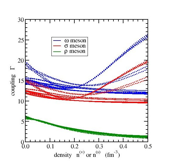
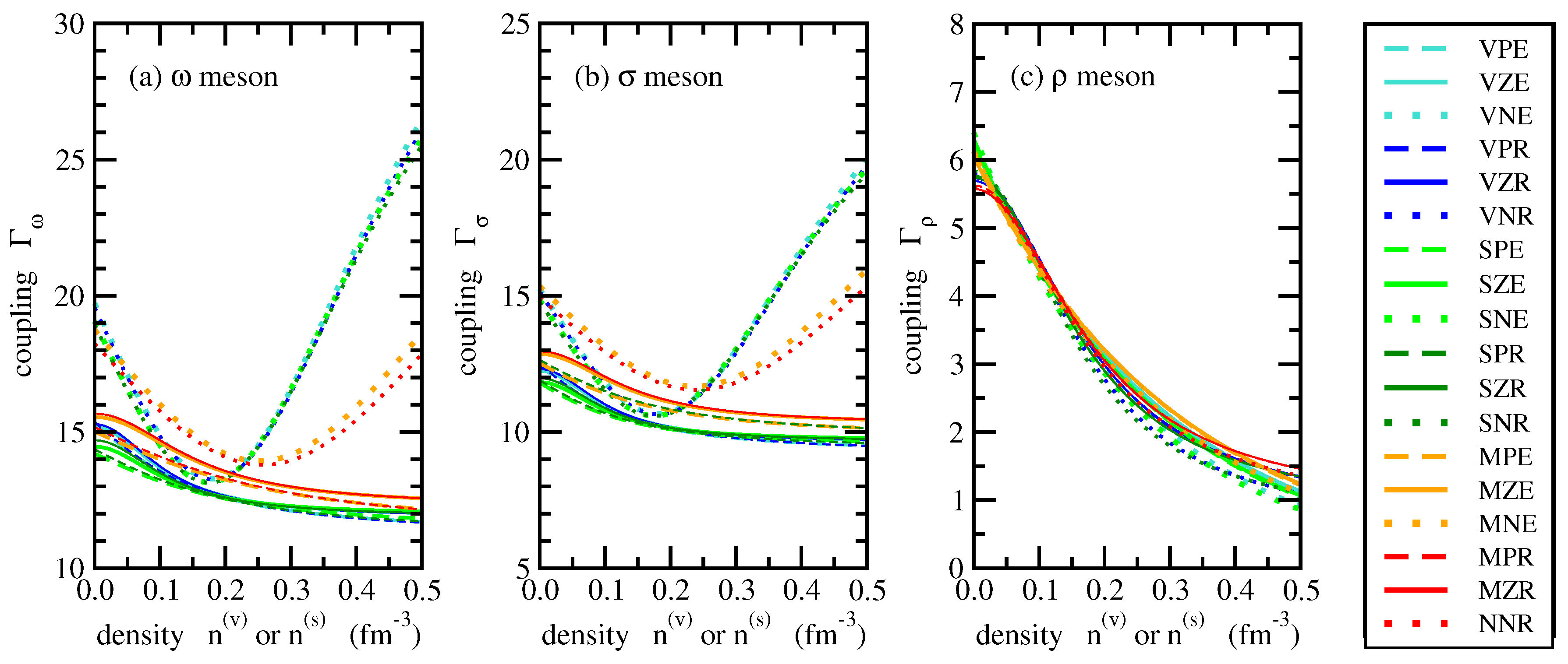
Larger differences between the parametrizations are seen when the density dependencies of the couplings are compared for a wide range of densities. The couplings of the , , and meson are depicted in Figure 1. The parametrizations of the meson couplings with and (full and dashed lines in Panel (a) of Figure 1) show a smooth decreasing trend with increasing density without a strong variation. In contrast, the functional form of for parametrizations with (dotted lines in Panel (a) of Figure 1) is very different with a minimum at densities slightly above the nuclear saturation density and a strong increase for larger densities, in particular for the vector (light and dark blue lines) and scalar (light and dark green lines) dependencies. A less strong increase is observed for a mixed dependency (orange and red lines). There is no strong influence on the meson coupling from the choice of the functional form of the meson coupling, whether exponential or rational.
The density dependencies of the meson couplings, depicted in Panel (b) of Figure 1, show a very similar pattern as the meson couplings. The main differences are the somewhat smaller absolute values. Again, the parametrizations with stick out with a rising trend of the couplings at high densities.
The density dependence of the meson couplings, shown in Panel (c) of Figure 1, is almost the same for all parametrizations. There is a slightly larger spread at densities above saturation, but in all cases, a decrease of the coupling with increasing density is obtained. The difference between the exponential and rational form of the functions can be recognized in the region close to zero density.
5. Properties of Nuclear Matter and Equation of State
Studying the EoS allows a further comparison of the different parametrizations. The nuclear matter parameters that characterize the EoS close to the saturation point and the EoS for symmetric matter and neutron matter can be examined. The density dependence of the symmetry energy is of particular interest for astrophysical applications.
5.1. Nuclear Matter Parameters
The energy per nucleon can be written as a power series:
in squares of the isospin asymmetry:
which depends on the difference between the neutron and proton vector densities. Here, the neutron-proton mass difference is neglected in the expansion. The first contribution in Equation (65) is the energy per nucleon in symmetric nuclear matter:
that only depends on the total baryon density:
It can be expanded close to the saturation point in powers of:
measuring the deviation from the saturation density . Similarly, the symmetry energy can be expanded as:
with explicit terms up to second order in x. The coefficients in Equation (67) are the average nucleon mass, , the binding energy per nucleon at saturation, , the incompressibility, K, and the skewness, Q. There is no term linear in x because the expansion is around the minimum of the energy in symmetric matter where the pressure vanishes. The coefficients in (70) are the symmetry energy at saturation, J, the slope parameter, L, and the symmetry incompressibility, . All coefficients can be obtained from appropriate derivatives of the energy per nucleon with respect to and at .
The six characteristic nuclear parameters together with the saturation density, , are presented in Table 3 for all 18 models of the present study. In addition, the average Dirac effective mass , cf. Equation (36), in symmetric nuclear matter and the average Landau effective mass , which is related to the density of states at the Fermi energy, are given in units of the average nuclear mass in a vacuum, . Here, the definition:
of the Landau effective mass with the Fermi momentum is used. The data are compared to average values, including uncertainty ranges, of more than 200 existing parametrizations of the Skyrme–Hartree–Fock (SHF) and RMF models collected in [3] and [5], respectively.
The scattering of the and values in the present RMF parametrizations is rather small, and the obtained data are consistent with the expectations from previous RMF models, but lower than the average value of SHF models. A larger spread is obtained for the incompressibilities, K, but their values are within the error bands of SHF and RMF models. A precise determination of K from fits to properties of nuclei seems to be difficult. A recent comprehensive analysis of experimental information on giant monopole resonances in [21] indicated an acceptable range of 250 MeV 315 MeV, which is on the high side of the values from the present fits. The values for the skewness Q span a wide range with a clear correlation with the sign of the parameters for the and meson, i.e., the constraint on the function (59) at zero density. This fact becomes even more evident when the correlation of the incompressibility K with the skewness Q is investigated as shown in Panel (a) of Figure 2. For and , the values of Q are the lowest of all parametrizations (diamonds), but for and , they are the highest (squares). The sets with and (circles) are in between. At the same time, there is a systematic trend of larger K values with smaller parameters. The large positive values for Q indicate that the EoS of symmetric matter will be rather stiff at high baryon densities. From the inspection of Table A1, Table A2 and Table A3, also a clear correlation of the mass of the meson with the sign of the parameter for is found. Negative values of prefer to be associated with the largest meson masses.
The different parametrizations predict symmetry energies at saturation J within a narrow range, similar as for the values. The data are close to the values expected from SHF and RMF models and inside the uncertainty band. The extracted slope parameters, L, cover a somewhat larger range that is more consistent with SHF parametrizations than the average of the RMF models. Certain trends can also be seen in the L-J correlation plot in Panel (b) of Figure 2. If models with exponential (E) and rational (R) density dependence of the meson are compared separately, there is an indication that values for L are systematically larger for models with pure scalar density dependence of the couplings and smaller for models with pure vector density dependence. Models with a mixed density dependence lie in between. On the other hand, there is the trend that ‘E’ models have on average a larger slope parameter L than ‘R’ models.
A large spread of the symmetry incompressibilities is seen in Table 3, and even the sign of cannot be determined unambiguously. Again, a systematic variation is observed as for the skewness Q or the slope parameter L. The obtained values for are consistent on the whole with those of the SHF and RMF models in the compilations. The Dirac and Landau effective masses at saturation, and , are systematically lower as compared to the averages of the RMF and SHF models. This observation is correlated with spin-orbit splittings that are predicted on average somewhat larger than in the experiment.
5.2. Equation of State and Symmetry Energy
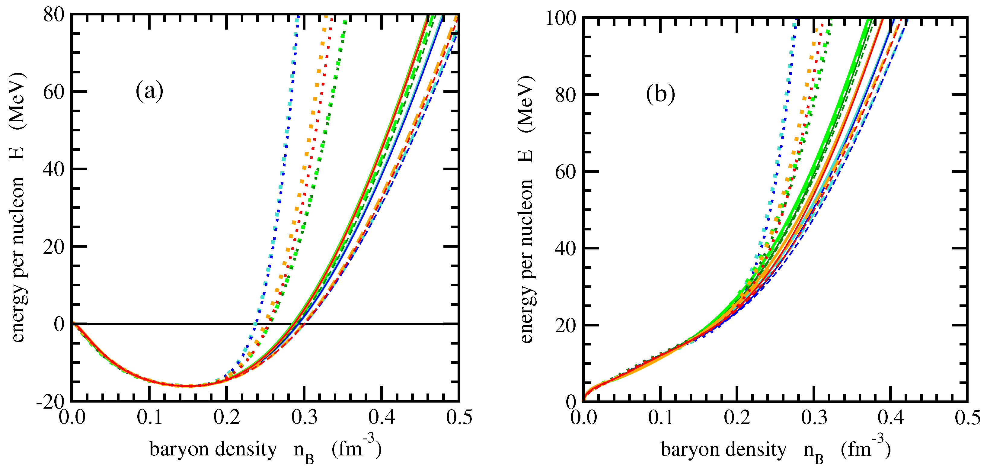
The different functional forms of the couplings, as depicted in Figure 1, also influence the equation of state. Here, we consider two cases for . The EoS of symmetric nuclear matter is shown in Panel (a) of Figure 3. For nucleon densities below approximately 0.2 fm, all parametrizations predict energies per baryon that are practically indistinguishable. Only at higher densities can different trends be seen. The most prominent feature is the large stiffness of parametrizations with negative and and the strong increase of the energy per nucleon with increasing density. This behavior is expected because of the high values of the skewness parameter Q, cf. Table 3. A similar observation is made for the case of pure neutron matter, shown in Panel (b) of Figure 3. The curves for parametrizations with negative again stick out because they are the stiffest. All other lines are within a band that corresponds to a softer neutron matter EoS. At densities below saturation, the curves are almost identical.
The density dependence of the symmetry energy is also easily extracted from the general EoS. It is depicted in Figure 4 for all parametrizations of the present work. There are only small differences between the curves for densities below approximately 0.12 fm. Larger variations are found at higher densities, but a different systematics is observed as compared to the EoS of symmetric matter or of neutron matter. Parametrizations with a pure dependence of the couplings on scalar densities predict the stiffest symmetry energy on average, whereas models with a vector densities dependence display the softest symmetry energies. This observation is consistent with the ordering of the models in Panel (b) of Figure 2. Parametrizations with larger values of J and L give stiffer symmetry energies; however, this is partly compensated by smaller values of the symmetry incompressibility .
The results clearly show that a fit of parametrizations to properties of finite nuclei fix the EoS at sub-saturation densities fairly well, but the extrapolation to higher densities depends strongly on the functional form of the couplings and the choice of the argument, i.e., whether a scalar or vector density dependence is used.
6. Constraints on the Density Dependence of the Couplings
The selection of a particular density as the argument of the couplings has also consequences for the EoS under specific conditions. This can serve as a criterion to exclude some parametrizations. Two particular cases can be distinguished: a dependence of the vector meson couplings on the scalar densities and a dependence of the scalar meson couplings on the vector densities. In the following, only symmetric matter is considered to keep the discussion simple.
Usually, the scalar densities and the Dirac effective masses are larger than zero. However, if the couplings depend on the total scalar density , there are solutions possible where and vanish at some finite total vector density . The couplings and thus the functions (30) in general have a smooth dependence on the density. The scalar potential (13) at zero scalar densities is given by the rearrangement term only as:
with the derivative (31) of the meson coupling function since in this case. If , the Dirac effective mass (36) becomes zero for , and there is a limiting (vector) density:
up to which the EoS can be calculated in the model for a particle i. This density is usually much larger than typical vector densities considered in applications of the model. However, in order to avoid the problem of a collapsing effective mass, the coupling of the meson should have a non-negative derivative at density zero, i.e., , if it depends on the scalar density. This condition would exclude parametrizations SPE, SNE, SPR and SNR.
Antiparticles contribute differently than particles to the vector and scalar densities (34) and (35), respectively. In the former case, their densities partly cancel, and in the latter case, they add to the total contribution of a particle species i (sum over ). For vanishing baryon densities, i.e., for all nucleons i, the effective chemical potentials have to vanish and the vector potentials and in Equation (14) are zero, as well. However, the scalar densities are positive at finite temperature and rise with increasing T. Hence, the scalar potential is finite. If the couplings of the scalar mesons depend on the total vector density , the vector potentials have a contribution from the rearrangement terms. For symmetric nuclear matter, they are given by:
with the derivative (45) of the meson coupling function. If the derivative is unequal zero, the chemical potential is finite and not zero as expected from the condition of vanishing vector densities. The mismatch between the conditions and becomes more severe with increasing temperature. This feature can be avoided by excluding the parametrizations VPE, VNE, VPR, VNR and VZE to guarantee that the derivative of the vector meson couplings are zero at vanishing total baryon density. The only the parametrization VZR is admitted.
The two problems above do not appear for the M parametrizations where the couplings of vector (scalar) mesons depend only on vector (scalar) densities. This form of modeling the effective in-medium interaction closely corresponds to the structure of most of the earlier RMF models with NL self-interactions of the mesons. In these approaches, there are no cross-terms of and contributions in the Lagrangian density. Only self-couplings of the form:
and:
were considered additionally in Equation (4), cf. [5]. This leads to field equations:
for the and mesons without a cross-coupling. Couplings of the form , which were introduced later in some models to modify the density dependence of the isovector part of the interaction, also do not violate the vector-scalar separation.
Taking the above considerations into account, only the SZE, SZR, VZR and all M parametrizations are really viable since they do not show the identified problems.
7. Conclusions and Outlook
Relativistic mean-field models are widely-used phenomenological approaches to describe the properties of nuclear matter and finite nuclei. Within a subclass of these models, i.e., those with density-dependent meson-nucleon couplings, the effects of choosing different functional forms of the dependence on vector or scalar particle densities were studied going beyond the standard choice of functions and assumed vector density dependence. The model parameters were obtained in all cases by a fit to observables of a selected set of spherical nuclei.
Despite the differences of the obtained energy density functionals, the description of nuclei has practically the same quality for all parametrizations, and the equations of state of symmetric nuclear matter and pure nuclear matter below the nuclear saturation density look very similar. In contrast, differences in some of the characteristic nuclear matter parameters and the equations of state above saturation are found. This is most evident for the incompressibility K and the skewness Q that correlate with the parameter of the rational function used for the density dependence of the isoscalar mesons. The differences in the nuclear matter parameters are reflected in the high-density behavior of the equations of state. Similarly, there is a connection between the symmetry energy at saturation J, the slope parameter L and the choice of the argument, i.e., scalar or vector density. This also affects the stiffness of the symmetry energy. Robust constraints at densities above nuclear saturation are clearly needed to select proper parametrizations for further applications of the model.
Some of the parametrizations studied in this work can lead to problems, e.g., the breakdown of the description of nuclear matter at a finite baryon density or the non-vanishing of the baryon chemical potential at finite temperature and zero baryon density. As a consequence, certain combinations of functional forms and arguments for the density dependence of the couplings have to be rejected, in particular those where the couplings of the vector mesons depend on the scalar density with negative derivative or couplings of scalar mesons depending on vector densities.
In the present study, only models with , and mesons were considered. In a next step, also the meson should be included, which could affect particularly the density dependence of the symmetry energy at high baryon densities. Furthermore, the effect of tensor couplings of the vector mesons with the nucleons could be investigated. In this study, no mechanism for taking care of pairing effects was included in the description. All these future extensions of the model will increase the number of independent parameters, and a more extensive fitting procedure is required. Furthermore, the selection of observables and the size of their uncertainties can be reconsidered and will affect the final predictions of the models.
Acknowledgments
This work was supported by “NewCompStar”, COST Action MP1304, and the DFG, Grant No. SFB1245.
Conflicts of Interest
The author declares no conflict of interest. The founding sponsors had no role in the design of the study; in the collection, analyses or interpretation of data; in the writing of the manuscript; nor in the decision to publish the results.
Abbreviations
The following abbreviations are used in this manuscript:
| DD | density dependent |
| EDF | energy density functional |
| EoS | equation of state |
| MF | mean-field |
| RMF | relativistic mean-field |
Appendix A
Explicit values of the mass of the meson, the reference densities, the meson couplings at the reference densities and the parameters of the functions (59) and (60) are given in Table A1, Table A2 and Table A3 for the three types of density dependence considered in this work. The parameters of the rational function (59) are not specified since they are determined by Relation (63).

Table A1.
Parameter sets from the fitting of DD-RMF models with different vector density dependencies of the couplings to observables of nuclei.
Table A1.
Parameter sets from the fitting of DD-RMF models with different vector density dependencies of the couplings to observables of nuclei.
| Quantity | Unit | VPE | VZE | VNE | VPR | VZR | VNR |
|---|---|---|---|---|---|---|---|
| (MeV) | 544.929443 | 545.650146 | 547.930176 | 545.250793 | 545.902039 | 547.892944 | |
| (fm) | 0.15125801 | 0.15137400 | 0.15110700 | 0.15093000 | 0.15105100 | 0.15081701 | |
| (fm) | 0.14202256 | 0.14204837 | 0.14106791 | 0.14173270 | 0.14174370 | 0.14084541 | |
| 12.972373 | 13.020596 | 13.496406 | 12.983727 | 13.045012 | 13.488939 | ||
| 0.57019352 | 1.46252795 | 0.68803968 | 0.54474910 | 1.44323308 | 0.67084499 | ||
| 0.84003228 | 1.87156006 | 0.23379376 | 0.80836122 | 1.86275602 | 0.23111957 | ||
| 0.62992869 | 0.00000000 | −1.19405109 | 0.64215022 | 0.00000000 | −1.20093918 | ||
| 10.407099 | 10.453366 | 10.826948 | 10.421222 | 10.475092 | 10.821014 | ||
| 0.79862873 | 1.65747024 | 0.63412221 | 0.75851162 | 1.62304354 | 0.61917590 | ||
| 1.16565166 | 2.11264687 | 0.23312610 | 1.11268608 | 2.08245333 | 0.23041316 | ||
| 0.53475515 | 0.00000000 | −1.19575973 | 0.54733478 | 0.00000000 | −1.20277872 | ||
| 3.7115331 | 3.7116771 | 3.5528619 | 3.6746919 | 3.6691670 | 3.5159609 | ||
| 0.52801299 | 0.51739597 | 0.58847803 | |||||
| 0.09405180 | 0.09647980 | 0.07125765 | |||||
| 0.70658221 | 0.70070777 | 0.76516974 | |||||
| 0.00000000 | 0.00000000 | 0.00000000 |
Table A2.
Parameter sets from the fitting of DD-RMF models with different scalar density dependencies of the couplings to observables of nuclei.
Table A2.
Parameter sets from the fitting of DD-RMF models with different scalar density dependencies of the couplings to observables of nuclei.
| Quantity | Unit | SPE | SZE | SNE | SPR | SZR | SNR |
|---|---|---|---|---|---|---|---|
| (MeV) | 545.769470 | 546.731262 | 549.089600 | 546.156250 | 547.086670 | 549.015686 | |
| (fm) | 0.15114300 | 0.15103699 | 0.150036011 | 0.15082000 | 0.15068200 | 0.14982501 | |
| (fm) | 0.14222754 | 0.14200704 | 0.14034841 | 0.14191435 | 0.14163363 | 0.14018976 | |
| 12.877718 | 12.961755 | 13.448970 | 12.906400 | 13.011437 | 13.442950 | ||
| 0.34433303 | 1.22405089 | 0.59939861 | 0.31660607 | 1.20055525 | 0.58959910 | ||
| 0.45505569 | 1.48060171 | 0.21432481 | 0.43186581 | 1.48483466 | 0.21315500 | ||
| 0.85586861 | 0.00000000 | 0.87854692 | 0.00000000 | ||||
| 10.359062 | 10.434348 | 10.817383 | 10.386197 | 10.475372 | 10.811744 | ||
| 0.77548245 | 1.52648887 | 0.55598902 | 0.67921564 | 1.45332485 | 0.54781176 | ||
| 1.02922672 | 1.86306504 | 0.21340776 | 0.92070349 | 1.80410166 | 0.21224707 | ||
| 0.56909379 | 0.00000000 | 0.60169926 | 0.00000000 | ||||
| 3.7855101 | 3.7817090 | 3.6446130 | 3.7468100 | 3.7345510 | 3.6057999 | ||
| 0.51056999 | 0.50244099 | 0.56340599 | |||||
| 0.09957897 | 0.10043021 | 0.078787928 | |||||
| 0.69330517 | 0.69129044 | 0.74509791 | |||||
| 0.00000000 | 0.00000000 | 0.00000000 |
Table A3.
Parameter sets from the fitting of DD-RMF models with different mixed density dependencies of the couplings to observables of nuclei.
Table A3.
Parameter sets from the fitting of DD-RMF models with different mixed density dependencies of the couplings to observables of nuclei.
| Quantity | Unit | MPE | MZE | MNE | MPR | MZR | MNR |
|---|---|---|---|---|---|---|---|
| (MeV) | 559.114136 | 565.282898 | 576.317200 | 559.953247 | 566.147888 | 574.627319 | |
| (fm) | 0.15099899 | 0.15085800 | 0.15096600 | 0.15069900 | 0.15058200 | 0.15068200 | |
| (fm) | 0.14191137 | 0.14158116 | 0.14108534 | 0.14160347 | 0.14129915 | 0.14094776 | |
| 13.578379 | 13.975589 | 14.915496 | 13.652579 | 14.043028 | 14.754153 | ||
| 0.19582295 | 0.72600089 | 0.28596668 | 0.19212490 | 0.71202843 | 0.26145579 | ||
| 0.27781695 | 0.92047055 | 0.11996222 | 0.27806993 | 0.91056398 | 0.11418520 | ||
| 1.09536788 | 0.00000000 | 1.09486950 | 0.00000000 | ||||
| 11.105234 | 11.513437 | 12.439312 | 11.174674 | 11.579861 | 12.281559 | ||
| 0.44211615 | 0.86901217 | 0.26729911 | 0.40997002 | 0.84117733 | 0.24893623 | ||
| 0.60234364 | 1.08798782 | 0.11847203 | 0.56723353 | 1.06039115 | 0.11436181 | ||
| 0.74390454 | 0.00000000 | 0.76658166 | 0.00000000 | ||||
| 3.7624700 | 3.7491491 | 3.6506290 | 3.7212999 | 3.7004030 | 3.6302810 | ||
| 0.48768699 | 0.47859299 | 0.51697201 | |||||
| 0.10766657 | 0.10917221 | 0.099700492 | |||||
| 0.67447743 | 0.67104831 | 0.69301708 | |||||
| 0.00000000 | 0.00000000 | 0.00000000 |
References
- Oertel, M.; Hempel, M.; Klähn, T.; Typel, S. Equations of state for supernovae and compact stars. Rev. Mod. Phys. 2017, 89, 015007. [Google Scholar] [CrossRef]
- Bender, M.; Heenen, P.H.; Reinhard, P.G. Self-consistent mean-field models for nuclear structure. Rev. Mod. Phys. 2003, 75, 121–180. [Google Scholar] [CrossRef]
- Dutra, M.; Lourenço, O.; Sá Martins, J.S.; Delfino, A.; Stone, J.R.; Stevenson, P.D. Skyrme Interaction and Nuclear Matter Constraints. Phys. Rev. 2012, C85, 035201. [Google Scholar] [CrossRef]
- Sellahewa, R.; Rios, A. Isovector properties of the Gogny interaction. Phys. Rev. 2014, C90, 054327. [Google Scholar] [CrossRef]
- Dutra, M.; Lourenço, O.; Avancini, S.S.; Carlson, B.V.; Delfino, A.; Menezes, D.P.; Providência, C.; Typel, S.; Stone, J.R. Relativistic Mean-Field Hadronic Models under Nuclear Matter Constraints. Phys. Rev. 2014, C90, 055203. [Google Scholar] [CrossRef]
- Lenske, H.; Fuchs, C. Rearrangement in the density dependent relativistic field theory of nuclei. Phys. Lett. 1995, B345, 355–360. [Google Scholar] [CrossRef]
- Fuchs, C.; Lenske, H.; Wolter, H.H. Density dependent hadron field theory. Phys. Rev. 1995, C52, 3043–3060. [Google Scholar] [CrossRef]
- Typel, S.; Wolter, H.H. Relativistic mean field calculations with density dependent meson nucleon coupling. Nucl. Phys. 1999, A656, 331–364. [Google Scholar] [CrossRef]
- Nikšić, T.; Vretenar, D.; Finelli, P.; Ring, P. Relativistic Hartree-Bogolyubov model with density dependent meson nucleon couplings. Phys. Rev. 2002, C66, 024306. [Google Scholar] [CrossRef]
- Long, W.H.; Meng, J.; Van Giai, N.; Zhou, S.G. New effective interactions in RMF theory with nonlinear terms and density dependent meson nucleon coupling. Phys. Rev. 2004, C69, 034319. [Google Scholar] [CrossRef]
- Lalazissis, G.A.; Nikšić, T.; Vretenar, D.; Ring, P. New relativistic mean-field interaction with density-dependent meson-nucleon couplings. Phys. Rev. 2005, C71, 024312. [Google Scholar] [CrossRef]
- Avancini, S.S.; Brito, L.; Chomaz, P.; Menezes, D.P.; Providência, C. Spinodal instabilities and the distillation effect in relativistic hadronic models. Phys. Rev. 2006, C74, 024317. [Google Scholar] [CrossRef]
- Gögelein, P.; van Dalen, E.N.E.; Fuchs, C.; Müther, H. Nuclear matter in the crust of neutron stars derived from realistic NN interactions. Phys. Rev. 2008, C77, 025802. [Google Scholar] [CrossRef]
- Typel, S.; Röpke, G.; Klähn, T.; Blaschke, D.; Wolter, H.H. Composition and thermodynamics of nuclear matter with light clusters. Phys. Rev. 2010, C81, 015803. [Google Scholar] [CrossRef]
- Roca-Maza, X.; Viñas, X.; Centelles, M.; Ring, P.; Schuck, P. Relativistic mean field interaction with density dependent meson-nucleon vertices based on microscopical calculations. Phys. Rev. 2011, C84, 054309. [Google Scholar] [CrossRef]
- Wang, M.; Audi, G.; Kondev, F.G.; Huang, W.; Naimi, S.; Xu, X. The AME2016 atomic mass evaluation (II). Tables, graphs and references. Chin. Phys. C 2017, 41, 030003. [Google Scholar] [CrossRef]
- Reinhard, P.G.; Rufa, M.; Maruhn, J.; Greiner, W.; Friedrich, J. Nuclear Ground State Properties in a Relativistic Meson Field Theory. Z. Phys. 1986, A323, 13–25. [Google Scholar] [CrossRef]
- Angeli, I.; Marinova, K. Table of experimental nuclear ground state charge radii: An update. Atom. Data Nucl. Data Tables 2013, 99, 69–95. [Google Scholar] [CrossRef]
- De Vries, H.; De Jager, C.W.; De Vries, C. Nuclear charge and magnetization density distribution parameters from elastic electron scattering. Atom. Data Nucl. Data Tables 1987, 36, 495–536. [Google Scholar] [CrossRef]
- Sonzogni, A. NuDat 2.6, National Nuclear Data Center, Brookhaven National Laboratory. Available online: http://www.nndc.bnl.gov/nudat2/ (accessed on 27 July 2017).
- Stone, J.R.; Stone, N.J.; Moszkowski, S.A. Incompressibility in finite nuclei and nuclear matter. Phys. Rev. 2014, C89, 044316. [Google Scholar] [CrossRef]
Figure 1.
Density dependence of the meson-nucleon coupling on the vector density or scalar density for the meson (a), meson (b) and meson (c). The coding of the lines is given in the legend on the right.
Figure 1.
Density dependence of the meson-nucleon coupling on the vector density or scalar density for the meson (a), meson (b) and meson (c). The coding of the lines is given in the legend on the right.

Figure 2.
Correlation of the incompressibility K with the skewness Q in (a) and of the symmetry energy J with the slope parameter L in (b).
Figure 2.
Correlation of the incompressibility K with the skewness Q in (a) and of the symmetry energy J with the slope parameter L in (b).
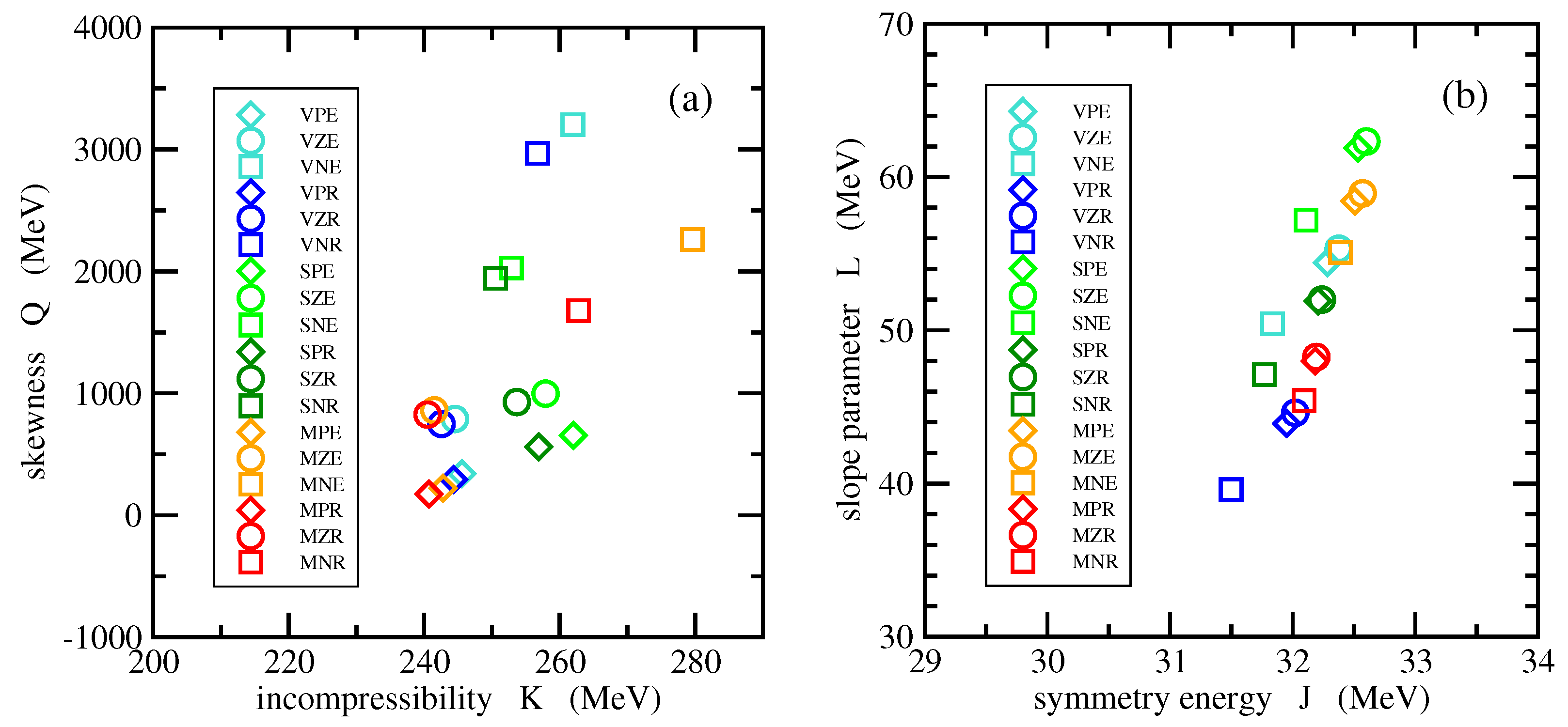
Figure 3.
Equation of state of symmetric nuclear matter in (a) and of pure neutron matter in (b) for . The coding of the lines is the same as in Figure 1.
Figure 3.
Equation of state of symmetric nuclear matter in (a) and of pure neutron matter in (b) for . The coding of the lines is the same as in Figure 1.

Figure 4.
Dependence of the symmetry energy on the baryon density. The coding of the lines is the same as in Figure 1.
Figure 4.
Dependence of the symmetry energy on the baryon density. The coding of the lines is the same as in Figure 1.
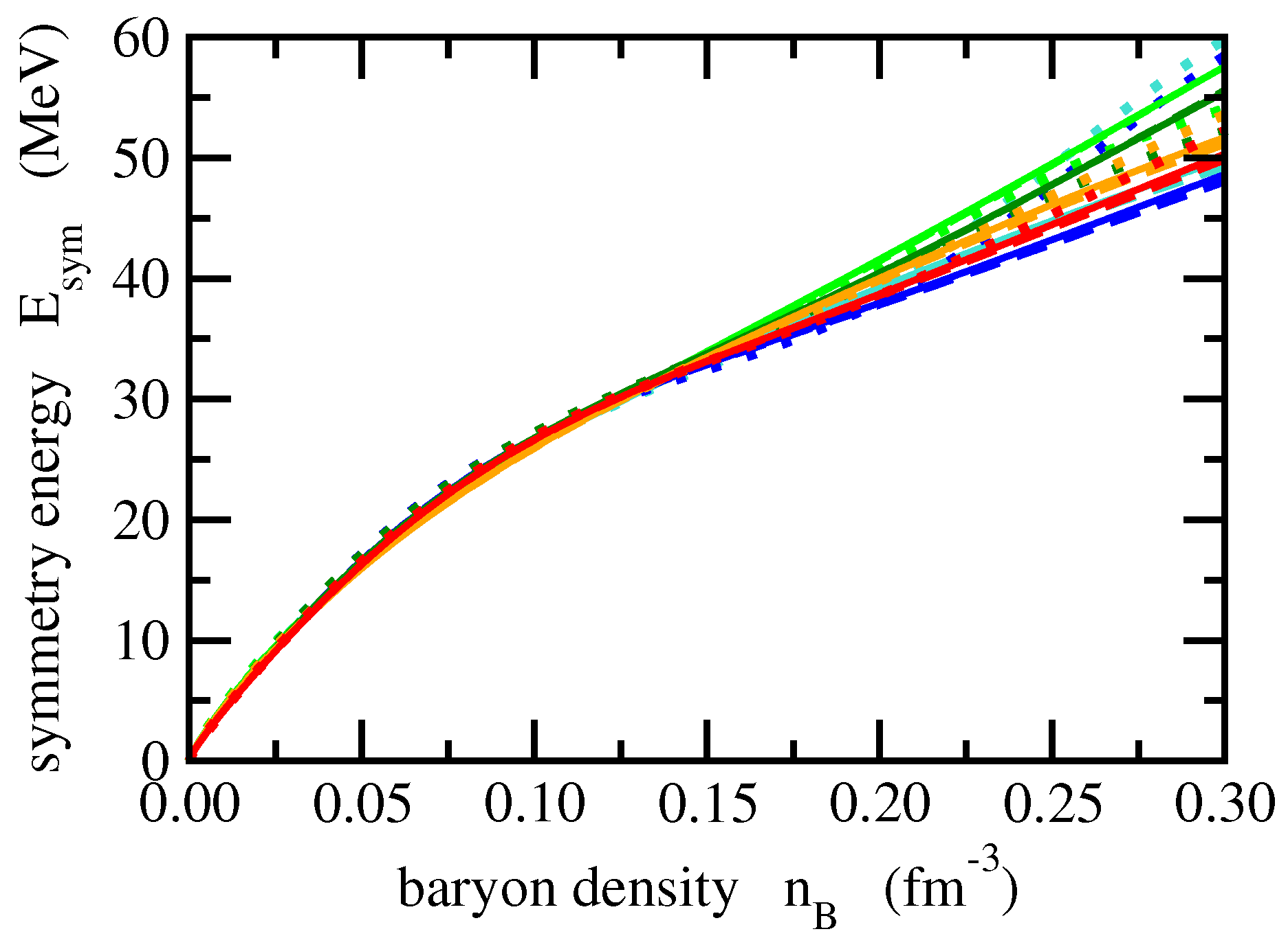
Table 1.
Selected nuclei and values of experimental observables used in the fitting procedure: binding energies per nucleon , charge radii , diffraction radii , surface thicknesses and spin-orbit splittings and for neutron and proton levels, respectively, with principal quantum number n and orbital angular momentum l. The last line gives the assumed uncertainties.
| Nucleus | (MeV) | (fm) | (fm) | (fm) | (MeV) | (MeV) |
|---|---|---|---|---|---|---|
| O | 7.976206 | 2.7013 | 2.7642 | 0.8508 | 6.18 (0p) | 6.32 (0p) |
| O | 7.039685 | − | − | − | − | − |
| Ca | 8.551303 | 3.4764 | 3.8495 | 0.9682 | − | − |
| Ca | 8.666686 | 3.4738 | 3.9633 | 0.8903 | 2.02 (1p), 8.39 (0f) | − |
| Ni | 8.642779 | − | − | − | 1.11 (0f), 7.16 (0f) | − |
| Ni | 8.682466 | − | − | − | − | − |
| Zr | 8.709969 | 4.2696 | 5.0399 | 0.9573 | − | 1.51 (1p) |
| Sn | 8.252974 | − | − | − | − | − |
| Sn | 8.522566 | 4.6103 | − | − | − | − |
| Sn | 8.354872 | 4.7093 | − | − | − | 1.48 (1d), 6.14(0g) |
| Ce | 8.376317 | 4.8770 | − | − | 0.475 (2p), 5.88 (0h) | − |
| Pb | 7.867453 | 5.5010 | 6.7760 | 0.9190 | 0.898 (2p) | 1.33 (1d), 5.55 (0h) |
| uncertainty | 0.01 | 0.01 | 0.005 | 0.1 | 0.1 |
Table 2.
Quality of the parametrizations measured with the quantities per number of degrees of freedom and the root-mean-square error of the binding energy.
Table 2.
Quality of the parametrizations measured with the quantities per number of degrees of freedom and the root-mean-square error of the binding energy.
| Parametrization | /N | (MeV) |
|---|---|---|
| VPE | 96.3 | 1.497 |
| VZE | 92.6 | 1.456 |
| VNE | 91.6 | 1.369 |
| VPR | 96.9 | 1.504 |
| VZR | 93.1 | 1.461 |
| VNR | 92.2 | 1.382 |
| SPE | 97.1 | 1.520 |
| SZE | 94.3 | 1.481 |
| SNE | 96.6 | 1.436 |
| SPR | 97.6 | 1.522 |
| SZR | 94.7 | 1.491 |
| SNR | 96.7 | 1.439 |
| MPE | 98.0 | 1.520 |
| MZE | 96.9 | 1.493 |
| MNE | 96.9 | 1.436 |
| MPR | 98.5 | 1.523 |
| MZR | 97.1 | 1.494 |
| MNR | 97.7 | 1.453 |
Table 3.
Nuclear matter parameters of the DD-RMF parametrizations determined in Section 4 in comparison with averages of Skyrme–Hartree–Fock (SHF) and RMF models.
Table 3.
Nuclear matter parameters of the DD-RMF parametrizations determined in Section 4 in comparison with averages of Skyrme–Hartree–Fock (SHF) and RMF models.
| Parameter Set | (fm) | (MeV) | K (MeV) | Q (MeV) | J (MeV) | L (MeV) | (MeV) | () | () |
|---|---|---|---|---|---|---|---|---|---|
| VPE | 0.15126 | 16.076 | 245.56 | 339.98 | 32.283 | 54.406 | −89.093 | 0.57610 | 0.63835 |
| VZE | 0.15137 | 16.058 | 244.54 | 789.59 | 32.375 | 55.316 | −82.197 | 0.57337 | 0.63592 |
| VNE | 0.15111 | 16.024 | 261.93 | 3203.71 | 31.836 | 50.421 | 20.421 | 0.54927 | 0.61420 |
| VPR | 0.15093 | 16.073 | 244.34 | 293.93 | 31.952 | 43.917 | −76.208 | 0.57631 | 0.63846 |
| VZR | 0.15105 | 16.053 | 242.56 | 749.43 | 32.021 | 44.612 | −70.045 | 0.57291 | 0.63542 |
| VNR | 0.15082 | 16.022 | 256.72 | 2969.10 | 31.498 | 39.611 | 37.600 | 0.55041 | 0.61515 |
| SPE | 0.15114 | 16.102 | 262.00 | 655.76 | 32.532 | 61.888 | −21.728 | 0.58713 | 0.64829 |
| SZE | 0.15104 | 16.077 | 257.90 | 998.37 | 32.601 | 62.321 | −24.294 | 0.58261 | 0.64418 |
| SNE | 0.15004 | 16.040 | 252.88 | 2028.14 | 32.109 | 57.186 | 29.789 | 0.55683 | 0.62069 |
| SPR | 0.15082 | 16.097 | 256.92 | 560.89 | 32.207 | 51.913 | −10.488 | 0.58637 | 0.64723 |
| SZR | 0.15068 | 16.069 | 253.78 | 929.49 | 32.238 | 52.002 | −12.901 | 0.58073 | 0.64238 |
| SNR | 0.14983 | 16.038 | 250.53 | 1942.60 | 31.769 | 47.103 | 50.326 | 0.55783 | 0.62153 |
| MPE | 0.15100 | 16.099 | 242.79 | 223.14 | 32.507 | 58.424 | −78.658 | 0.58042 | 0.64218 |
| MZE | 0.15086 | 16.085 | 241.49 | 861.46 | 32.570 | 58.925 | −70.031 | 0.57331 | 0.63572 |
| MNE | 0.15097 | 16.091 | 279.57 | 2261.71 | 32.390 | 55.086 | −36.126 | 0.55375 | 0.61817 |
| MPR | 0.15070 | 16.093 | 240.71 | 173.89 | 32.184 | 48.000 | −71.984 | 0.57911 | 0.64092 |
| MZR | 0.15058 | 16.079 | 240.50 | 826.01 | 32.193 | 48.254 | −62.835 | 0.57216 | 0.63462 |
| MNR | 0.15068 | 16.088 | 262.79 | 1678.00 | 32.093 | 45.411 | −35.555 | 0.55747 | 0.62144 |
| SHF av.[3] | 0.160 ± 0.005 | 15.96 ± 0.31 | 246 ± 41 | −328 ± 158 | 31.2 ± 6.7 | 41.9 ± 36.1 | −186 ± 127 | 0.830 ± 0.143 | |
| RMF av. [5] | 0.152 ± 0.008 | 16.13 ± 0.51 | 271 ± 86 | −160 ± 710 | 33.4 ± 4.7 | 91.2 ± 24.3 | 11 ± 83 | 0.668 ± 0.086 |
© 2018 by the author. Licensee MDPI, Basel, Switzerland. This article is an open access article distributed under the terms and conditions of the Creative Commons Attribution (CC BY) license (http://creativecommons.org/licenses/by/4.0/).
Share and Cite
MDPI and ACS Style
Typel, S. Relativistic Mean-Field Models with Different Parametrizations of Density Dependent Couplings. Particles 2018, 1, 3-22. https://doi.org/10.3390/particles1010002
AMA Style
Typel S. Relativistic Mean-Field Models with Different Parametrizations of Density Dependent Couplings. Particles. 2018; 1(1):3-22. https://doi.org/10.3390/particles1010002
Chicago/Turabian StyleTypel, Stefan. 2018. "Relativistic Mean-Field Models with Different Parametrizations of Density Dependent Couplings" Particles 1, no. 1: 3-22. https://doi.org/10.3390/particles1010002