Lee–Yang Zeroes in the Baryon Fugacity Plane: The Role of High Densities

Abstract

We compute the canonical partition functions and the Lee–Yang zeros in $N_f=2$ lattice QCD at temperature $T=1.20T_c$ lying above the Roberge–Weiss phase transition temperature $T_{RW}$. The phase transition is characterized by the discontinuities in the baryon number density at specific values of imaginary baryon chemical potential. We further develop our method to compute the canonical partition functions using the asymptotic expression for respective integral. Then, we compute the Lee–Yang zeros and study their behavior in the limit of high baryon density.

1. Introduction

The properties of the QCD phase diagram in the temperature-baryon chemical potential plane are studied both experimentally and theoretically very intensively; see, e.g., [1,2,3,4]. The current experiments at RHIC (BNL) and LHC (CERN), and the future experiments at FAIR (GSI) and NICA (JINR), are devoted to such studies. Lattice QCD is a first principles theoretical approach to study the nonperturbative properties of QCD. It proved to be a very powerful method to study QCD at zero baryon chemical potential ${\mu }_B$. At nonzero ${\mu }_B$, the standard Monte Carlo methods are not applicable due to a severe sign problem. Various approaches to bypass this problem are under development with partial successes. These include reweighting, Taylor expansion, analytic continuation, canonical approach, strong coupling/dual methods, the density of states, and complex Langevin; see for review, e.g., [5,6]. Thanks to recent developments, one can access the regions at finite T and ${\mu }_B$ up to ${\mu }_B/T\sim 3$; see, e.g., [7,8,9]. But the task of locating the critical endpoint still remains unsolved.

In our work, we follow the canonical approach suggested in Ref. [10]. For imaginary chemical potential, i.e., for ${\mu }_B=i{\mu }_I$, the sign problem is absent since the fermion determinant is positive. For this reason, it is possible to use standard Monte Carlo algorithms to compute (imaginary) baryon density ${\rho }_B$ and other observables; see, e.g., [11,12,13,14]. Then, the canonical partition functions $Z_C(n,T,V)$ can be computed and, as a result, the grand partition function, $Z_{GC}$, can be evaluated at any complex value of the chemical potential, including physically relevant real values. The properties of QCD at imaginary chemical potential were first formulated in Ref. [15]. It was shown that $Z_{GC}$ is a periodic function of ${\mu }_I$ and at high enough temperature (above $T=T_{RW}$) the free energy has cusps at ${\mu }_I/T=\pi +2\pi k,k=0,\pm 1,...$. This leads to discontinuities in the imaginary baryon number density signaling the first-order phase transition.

Discontinuities in the baryon-number density emerge at the points where the pressure $p\left(\theta \right)$ loses analyticity and, therefore, $Z_{GC}\left(\xi \right)$ vanishes. These points are accumulated on the lines, which tend to the cuts of the baryon-number density in the complex chemical-potential plane; evidence for this scenario comes from the same arguments as in [16,17].

The values of $\xi$ where $Z_{GC}\left(\xi \right)=0$ are called Lee–Yang zeros (LYZ); they were introduced in Refs. [16,17] by T.D. Lee and C.-N. Yang. They discussed the idea of how the non-analyticity of phase transitions can appear in the thermodynamic limit. The idea was to consider the truncated series of $Z_{GC}(\theta ,T,V)$ in terms of fugacity ${\xi }_B=e^{{\mu }_B/T}=e^{\theta }$. The truncated series becomes a polynomial whose zeros (Lee–Yang zeros) completely determine the phase structure of the theory. For this reason, the study of LYZ in QCD is an interesting and important task, and their properties were studied in a number of works by means of lattice QCD approach [18,19] or in effective QCD models [20,21,22].

After the pioneering work by Roberge and Weiss [15], where they pointed out the relation between imaginary chemical potential and the phases of QCD, the phase structure of the complex chemical-potential plane was thoroughly studied numerically [11], and the location of discontinuities of the baryon-number density as well as the consistency of the respective canonical partition functions with the experimental data were found [23].

The underlying reason for a particular arrangement of Lee–Yang zeroes in QCD and its dependence on the temperature is the subject of further studies.

In a number of papers [19,24,25], we developed methods to compute the canonical partition functions $Z_C(n,T,V)$ using the lattice data for imaginary baryon density ${\rho }_B$ at both low and high temperatures. In particular, in Ref. [25] using the stationary phase method we suggested the solution of the problem of computation of $Z_C(n,T,V)$ for temperatures above the Roberge–Weiss transition [15] when the imaginary baryon density has discontinuity and successfully applied this new method to the case of $T=1.35T_c$. At this temperature, the baryon density is described by the polynomial of degree three.

We demonstrated in Ref. [25] that $Z_C(n,T,V)$ computed using this method allow one to reproduce the input expression for the baryon number density and, moreover, allow one to obtain the correct Lee–Yang zeros pattern corresponding to the first-order Roberge–Weiss transition. Here, we improve our method using higher-order approximation for the stationary phase method to compute $Z_C(n,T,V)$ and apply it to the case of $T=1.20T_c>T_{RW}$ when one needs to use a higher degree polynomial to describe lattice data for imaginary baryon density.

In this work, we study the arrangement of the Lee–Yang zeroes in the complex fugacity plane and the respective discontinuities of the net baryon-number density in the complex chemical-potential plane (along the lines ${\theta }_I=2\pi n,n\in Z$) in more detail.

The paper is organized as follows. In Section 2, we describe the improvements in computation of $Z_C(n,T,V)$ and demonstrate their effect. In Section 3, the results for the Lee–Yang zeros are presented. We discuss the difference in their behavior compared to the higher temperature case. In Section 4, we present our conclusions.

2. Computation of the Canonical Partition Functions

It is useful to introduce notation $Z_n$ for the normalized canonical partition function, $Z_C(n,T,V)/Z_C(0,T,V)$. The pressure p and the baryon number density $\rho$ are defined as follows:

$$p=\frac{T}{V}ln{Z}_{GC}(\theta ,T,V),$$

(1)

$$\rho =\frac{N_B}{V}=\frac{1}{T}\frac{\partial p}{\partial \theta },$$

(2)

where $\theta ={\mu }_B/T$, $N_B$ is the net baryon number in the lattice volume. In the complex $\theta$ plane, it is convenient to use notations $\theta ={\theta }_R+ı{\theta }_I$ and $\rho ={\rho }_R+ı{\rho }_I$. We also need the dimensionless variables $\widehat{\rho }=\rho /T^3={\widehat{\rho }}_R+ı{\widehat{\rho }}_I$.

It is known that $T>T_{RW}$${\rho }_I\left({\theta }_I\right)$ can be well approximated by an odd-power polynomial [24,26]. In this paper, we use numerical results for imaginary baryon number density at $T=1.20T_c>T_{RW}$. These numerical results are slightly different from those we presented before in Ref. [24] due to increased statistics. In Ref. [24], we fitted the lattice data for imaginary baryon number density by the polynomial of degree five

$${\widehat{\rho }}_I\left({\theta }_I\right)\simeq a_1{\theta }_I-a_3{\theta }_I^3+a_5{\theta }_I^5,\left|{\theta }_I\right|<\pi .$$

(3)

For this fit, we find $a_1=0.4901\left(6\right),a_3=0.0132\left(3\right),a_5=-0.00016\left(2\right)$. For real chemical potential, Equation (3) implies

$${\widehat{\rho }}_R=a_1{\theta }_R+a_3{\theta }_R^3+a_5{\theta }_R^5.$$

(4)

Negative $a_5$ implies unphysical behavior at large chemical potential if higher terms in (4) are absent. For this reason, we decided to also use another fit of the lattice data:

$${\widehat{\rho }}_I\left({\theta }_I\right)\simeq a_1{\theta }_I-a_3{\theta }_I^3-a_7{\theta }_I^7,\left|{\theta }_I\right|<\pi .$$

(5)

corresponding to

$${\widehat{\rho }}_R=a_1{\theta }_R+a_3{\theta }_R^3+a_7{\theta }_R^7.$$

(6)

We obtained positive $a_7=1.43\times {10}^{-5}\left(13\right)$ for the fit (5) and slightly different $a_1$ and $a_3$: $a_1=0.49006\left(42\right),a_3=0.01360\left(13\right)$.

For this fit, the real baryon number density in Equation (6) is positive for all values of ${\theta }_R$. Below, we present our results for the fit (5) and make a brief comparison with the results obtained for the fit (3). We show our data for the imaginary baryon number density, which fit (3) and (5) in Figure 1. The difference between the fits is not seen by eye. Let us note that the behavior of ${\rho }_I$ seen in Figure 1 implies that it has discontinuity at ${\theta }_I=\pi$ since it is an odd periodic function of ${\theta }_I$ with period $2\pi$, as we discussed in the Introduction.

Given coefficients $a_i$, we can find the pressure up to the integration constant and, therefore, $Z_{GC}(\theta ,T,V)$ up to a factor. Then, we can compute the canonical partition functions by performing the Fourier transform

$$Z_C(n,T,V)={\int }_{-\pi }^{\pi }\frac{d{\theta }_I}{2\pi }{e}^{ın{\theta }_I}{Z}_{GC}(\theta =ı{\theta }_I,T,V)$$

(7)

numerically.

Before we proceed, we need to introduce some notations. We introduce the dimensionless quantity $\nu =V{T}^3$ characterizing the volume (the expression for $\nu$ in terms of lattice parameters has the form $\nu =N_s^3{N}_t^{-3}$). We also introduce the variable ${\displaystyle \varrho =\frac{n}{V{T}^3}}$, where n is the net baryon number of a particular physical state. This variable can help one to remember that the canonical partition functions $Z_C(n,T,V)$ correspond to the respective baryon number density $\varrho$. In what follows, $\varrho$ is called a particular density, in contrast to the grand-canonical ensemble average density $\rho$.

In Ref. [24], we demonstrated that using Equations (1)–(7) it is possible to compute $Z_n$ at temperature above $T_{RW}$ only for n below some $n_{max}$. The value of $n_{max}$ is estimated from the following condition: the sign of the canonical partition functions $Z_C(n,T,V)$ calculated by Formula (7) alternates at $n>n_{max}$. Negative values of $Z_C(n,T,V)$ (and, therefore, $Z_n$) are unphysical and indicate that our fit-function is not suitable. That is, it cannot describe high-density ($n/\nu >{\varrho }_{max}=n_{max}/\nu$) contributions to $Z_{GC}(\theta ,T,V)$. It should be noticed that $n_{max}$ depends significantly on the volume, whereas the respective density ${\varrho }_{max}$ depends on the volume only weakly and is in the region of $1.6$ at $T=1.35T_c$.

In Ref. [25], we explained the reason for this problem and found its solution. The unphysical negative values of $Z_n$ stem from the unphysical condition that the finite-volume system under study undergoes during a phase transition, implicitly imposed by combining the $2\pi -$periodicity of ${\rho }_I\left({\theta }_I\right)$ with the Equation (3). Actually, the function (3) is discontinuous at ${\theta }_I=\pi +2\pi k,k=\pm 1,\pm 2,...$. It should be emphasized that with $Z_n,n<n_{max}$ evaluated in [24], we reproduced the dependence of the net baryon-number density $\widehat{{\rho }_I}$ on ${\theta }_I$ for all ${\theta }_I$ except for small neighborhoods of the points ${\theta }_I=2\pi n,n\in Z$.

For this reason, the right-hand side of Equation (3) has to be modified near the Roberge–Weiss transition at ${\theta }_I=\pi$. This modification should depend on the volume and involve discontinuities of the type (3) in the infinite-volume limit only. To evaluate the net baryon-number density $\rho$ in a very close vicinity of the transition point ${\theta }_I=\pi$ presents a challenge. In Ref. [25], we suggested another approach. We employed an approximate analytical expression for $Z_n$ originally introduced in [15]. In this study, we further develop our ideas formulated in Ref. [25] and demonstrate that the improved approximation has the needed behavior near ${\theta }_I=\pi$ and adequately reproduces density (3) in the infinite-volume limit.

It should be emphasized that the problem of negative canonical partition functions $Z_C(n,T,V)<0$ is associated with the asymptotic regime when $\nu$ is fixed, $n\to \infty$ ($\varrho \to \infty$); however, a detailed study of high densities in the finite-volume case should be the subject of a separate study. Here, we consider two other asymptotic regimes: (i) $\nu \to \infty$, n is fixed ($\varrho \to 0$) and (ii) $\nu \to \infty$, $n\to \infty$ ($\varrho$ is fixed).

In the latter regime, the approach to obtain approximate expressions for the canonical partition functions in the case when $a_i=0$ for $i>3$ was formulated in Ref. [15]. Here, we consider the case when $a_1\ne 0$, $a_3\ne 0$, and $a_7\ne 0$. Thus, we evaluate the quantities

$$Z_{nA}=\frac{{\int }_{-ı\pi }^{ı\pi }d\theta e^{\nu F_n\left(\theta \right)}}{{\int }_{-ı\pi }^{ı\pi }d\theta e^{\nu F_0\left(\theta \right)}},where{F}_n\left(\theta \right)=-\varrho \theta +\frac{1}{2}{a}_1{\theta }^2+\frac{1}{4}{a}_3{\theta }^4+\frac{1}{8}{a}_7{\theta }^8,$$

(8)

applying the stationary phase method [27]. Let us note that the integrals in Equation (8) are computed along the imaginary axis, while the saddle point ${\theta }_s$ is real, as is shown in Figure 2. For this reason, we deform contour $AD$ to $ABCD$.

In our case, we use the stationary phase method for $\nu \to \infty$. The saddle point $\theta ={\theta }_s={\theta }_s\left(\varrho \right)$ is determined from the equation

$$a_7{\theta }^7+a_3{\theta }^3+a_1\theta -\varrho =0.$$

(9)

We note that dependence of ${\theta }_s$ on $\varrho$ is implied below though not explicitly indicated.

That is, we rearrange the integral in the numerator of (8) as follows:

$$\begin{array}{ccc}\hfill {\int }_A^D{e}^{\nu F_n\left(\theta \right)}d\theta & \to & {\int }_A^B{e}^{\nu F_n\left(\theta \right)}d\theta +{\int }_B^C{e}^{\nu F_n\left(\theta \right)}d\theta +{\int }_C^D{e}^{\nu F_n\left(\theta \right)}d\theta \hfill \\ \hfill & =& {\int }_0^{{\theta }_s}{e}^{\nu h_{-}({\theta }_R,\varrho )}d{\theta }_R+{\int }_{-\pi }^{\pi }{e}^{\nu f({\theta }_I,\varrho )}d{\theta }_I-{\int }_0^{{\theta }_s}{e}^{\nu h_{+}({\theta }_R,\varrho )}d{\theta }_R.\hfill \end{array}$$

(10)

We use the substitution $\theta ={\theta }_s+ı{\theta }_I$ to rearrange the integral over $BC$ into the second term in the lower row of formula (10), where the function $f({\theta }_I,\varrho )$ has the form

$$\begin{array}{ccc}\hfill f({\theta }_I,\varrho )& =& -\varrho {\theta }_s+\frac{1}{2}{a}_1{\theta }_s^2+\frac{1}{4}{a}_3{\theta }_s^4+\frac{1}{8}{a}_7{\theta }_s^8+b_2{\theta }_I^2+b_4{\theta }_I^4+b_6{\theta }_I^6+b_8{\theta }_I^8+i\alpha ,\hfill \end{array}$$

(11)

with

$$\begin{array}{ccc}\hfill b_2& =& -\frac{1}{2}\left(a_1+3a_3{\theta }_s^2+7a_7{\theta }_s^6\right),\hfill \\ \hfill b_4& =& \phantom{-}\frac{1}{4}\left(a_3+35a_7{\theta }_s^4\right),\hfill \\ \hfill b_6& =& -\frac{1}{2}7a_7{\theta }_s^2,\hfill \\ \hfill b_8& =& \phantom{-}\frac{a_7}{8},\hfill \\ \hfill \alpha & =& -{\theta }_I^3{\theta }_s\left(a_3+a_7\left({\theta }_I^4-7{\theta }_I^2{\theta }_s^2+7{\theta }_s^4\right)\right).\hfill \end{array}$$

(12)

Furthermore, we transform the integrals over $AB$ and $CD$ using, respectively, the substitutions $\theta ={\theta }_R-ı\pi$ and $\theta ={\theta }_R+ı\pi$ and obtain for functions $h_{\pm }({\theta }_R,\varrho )$

$$\begin{array}{ccc}\hfill h_{\pm }({\theta }_R,\varrho )& =& \frac{a_1}{2}\left({\theta }_R^2-{\pi }^2\right)+\frac{a_3}{4}\left({\theta }_R^4-6{\theta }_R^2{\pi }^2+{\pi }^4\right)\hfill \\ & +& \frac{a_7}{8}\left({\theta }_R^8-28{\pi }^2{\theta }_R^6+70{\pi }^4{\theta }_R^4-28{\pi }^6{\theta }_R^2+{\pi }^8\right)\hfill \\ & -& \varrho {\theta }_R\mp i\pi \varrho \pm i\pi {\theta }_R\left(a_1+a_3\left({\theta }_R^2-{\pi }^2\right)+a_7\left({\theta }_R^6-7{\pi }^2{\theta }_R^4+7{\pi }^4{\theta }_R^2-{\pi }^6\right)\right).\hfill \end{array}$$

(13)

The sum of the first and the third terms in Equation (10) should be omitted for the following reason. The baryon number density and, therefore, $F_n\left(\theta \right)$ are holomorphic functions over the interior of the rectangle $ABCD$ and, to employ the stationary phase method, we should keep them continuous over the rectangle $ABCD$ with its boundary (the periodicity of the baryon-number density under consideration requires that discontinuities emerge along the lines $AB$ and $CD$). Thus, we have to choose the values $F_n\left(\theta \right)$ on the segments $AB$ and $CD$ as limiting values when $\theta$ tends to the boundaries $AB$ and $CD$ from the interior of the rectangle $ABCD$ so that $F_n\left(\theta \right)$ is continuous and thus non-periodic. This being so, $F_n\left(\theta \right)=h_{+}({\theta }_R,\varrho )$ on $CD$ and $F_n\left(\theta \right)=h_{-}({\theta }_R,\varrho )$ on $AB$, where $h_{\pm }({\theta }_R,\varrho )$ are given by formula (13). It is evident from Equation (13) that $\mathrm{Re}{h}_{+}({\theta }_R,\varrho )=\mathrm{Re}{h}_{-}({\theta }_R,\varrho )$. This means that the first and the third terms in the upper row of formula (10) do not cancel each other, their sum is the product of the exponent $exp\left(\nu \mathrm{Re}{h}_{+}({\theta }_R,\varrho )\right)$ and the rapidly oscillating function $2ısin\left(\nu \mathrm{Im}{h}_{+}({\theta }_R,\varrho )\right)$. Thus, the sum of integrals ${\int }_A^B+{\int }_C^D$ is purely imaginary and can be omitted since the integrals both in the numerator and denominator of formula (8) are real. Therefore, the sum ${\int }_A^B+{\int }_C^D$ just cancels the imaginary part of the integral ${\int }_B^C$.

The second term in Equation (10) can be estimated using the asymptotic expansion of the integral

$$I={\int }_{-a}^{a}exp(-\lambda x^2)\phi (x;\lambda )dx,$$

(14)

in the limit $\lambda \to \infty$:

$${\int }_{-a}^{a}exp(-\lambda x^2)\phi (x;\lambda )dx\simeq \frac{1}{\sqrt{\lambda }}\sum _{k=0}^{\infty }{c}_{2k}\left(\lambda \right)\frac{\Gamma (k+1/2)}{{\lambda }^k},$$

(15)

where in some neighborhood of the origin the function $\phi (x;\lambda )$ meets the Taylor expansion $\phi (x;\lambda )={\sum }_{n=0}^{\infty }{c}_n\left(\lambda \right)x^n$, with coefficients $c_n\left(\lambda \right)$ remaining finite in the limit $\lambda \to \infty$. The validity of Equation (15) for the estimate under consideration can be proven by replacing ${\theta }_I=x{\nu }^{-1/3}$. This substitution gives rise to

$$\begin{array}{c}\hfill {\int }_{-\pi }^{\pi }{e}^{\nu f({\theta }_I,\varrho )}d{\theta }_I=\frac{1}{{\nu }^{\frac{1}{3}}}exp\left(\nu \left(-\varrho {\theta }_s+\frac{1}{2}{a}_1{\theta }_s^2+\frac{1}{4}{a}_3{\theta }_s^4+\frac{1}{8}{a}_7{\theta }_s^8\right)\right)\mathcal{R}(\varrho ,\nu ),\end{array}$$

(16)

where

$$\begin{array}{ccc}\hfill \mathcal{R}(\varrho ,\nu )& =& {\int }_{-\pi \sqrt[3]{\nu }}^{\pi \sqrt[3]{\nu }}dxexp\left\{-\frac{{\nu }^{1/3}}{2}\left(a_1+3a_3{\theta }_s^2+7a_7{\theta }_s^6\right)x^2\right\}\hfill \\ & \times & exp\left\{\frac{1}{{\nu }^{1/3}}\frac{1}{4}\left(a_3+35a_7{\theta }_s^4\right)x^4-\frac{1}{\nu }\frac{7}{2}{a}_7{\theta }_s^2{x}^6+\frac{1}{{\nu }^{5/3}}\frac{1}{8}{a}_7{x}^8\right\}\hfill \\ & \times & cos\left\{\left(a_3+a_7\left(\frac{1}{{\nu }^{4/3}}{x}^4-\frac{1}{{\nu }^{2/3}}7x^2{\theta }_s^2+7{\theta }_s^4\right)\right){\theta }_s{x}^3\right\},\hfill \end{array}$$

(17)

and the function $\phi$ from Equation (15) is provided by the second and third rows of Equation (17).

Now, it is a straightforward matter to obtain the sought-for asymptotic expansion.

$$\begin{array}{ccc}\hfill \mathcal{R}(\varrho ,\nu )& =& \sqrt{\frac{\pi }{{\displaystyle \ell {\nu }^{1/3}}}}\left(1+\frac{3}{16\nu {\ell }^2}\left(a_3+35a_7{\theta }_s^4-\frac{5{\theta }_s^2}{\ell }{(a_3+7a_7{\theta }_s^4)}^2\right)+\underline{O}\left(\frac{1}{{\nu }^2}\right)\right),\hfill \end{array}$$

(18)

where

$$\begin{array}{ccc}\hfill \ell & =& \frac{1}{2}\left(a_1+3a_3{\theta }_s^2+7a_7{\theta }_s^6\right).\hfill \end{array}$$

(19)

Finally, our approximation $Z_{nA}$ for the normalized canonical partition functions is

$$Z_{nA}=\frac{e^{\nu f(0,\varrho )}}{e^{\nu f(0,0)}}\frac{\mathcal{R}(\varrho ,\nu )}{\mathcal{R}(0,\nu )}.$$

(20)

Equation (20) corresponds to the next-to-next-to-leading approximation in the asymptotic expansion (16). It provides better approximation for $Z_{nA}$ than the values obtained in the leading approximation (first factor in Equation (20)) or in the next-to-leading approximation (first term in Equation (18)), as follows from the results for the baryon number density presented below. These approximations are denoted below as third-order, second-order, and first-order approximations.

To demonstrate the quality of the approximation $Z_{nA}$, we computed the real and imaginary baryon number density using expressions

$$\begin{array}{ccc}\hfill {\widehat{\rho }}_R& =& \frac{1}{\nu }\frac{2{\sum }_{n>0}n{Z}_{nA}sinh\left(n{\theta }_R\right)}{1+2{\sum }_{n>0}{Z}_{nA}cosh\left(n{\theta }_R\right)},\hfill \end{array}$$

(21)

$$\begin{array}{ccc}\hfill {\widehat{\rho }}_I& =& \frac{1}{\nu }\frac{2{\sum }_{n>0}n{Z}_{nA}sin\left(n{\theta }_I\right)}{1+2{\sum }_{n>0}{Z}_{nA}cos\left(n{\theta }_I\right)},\hfill \end{array}$$

(22)

and compared them with input densities (6) and (5). We present respective relative deviations in Figure 3, Figure 4 and Figure 5. One can see from the left panels of Figure 3 and Figure 4 that the relative deviation of ${\widehat{\rho }}_I$ is substantially reduced when we improve the approximation for $Z_{nA}$ from the first approximation to the third approximation. We should note that we did not include the very vicinity of ${\theta }_I=\pi$ in these figures. When ${\theta }_I$ is very close to $\pi$, the functions (5) and (22) are intrinsically different for any finite volume. The agreement between the input ${\widehat{\rho }}_I$ and approximated ${\widehat{\rho }}_I$ becomes even better when we move from $V={16}^3$ to $V={40}^3$, as follows from comparison of Figure 3 and Figure 4. This effect is emphasized in the left panel of Figure 5.

For the relative deviation of ${\widehat{\rho }}_R$ shown in the right panels of same figures, we see qualitatively the same behavior with some differences. The second and third approximations provide more or less the same precision, which is much better than the precision of the first approximation. Increasing the volume also improves precision very much.

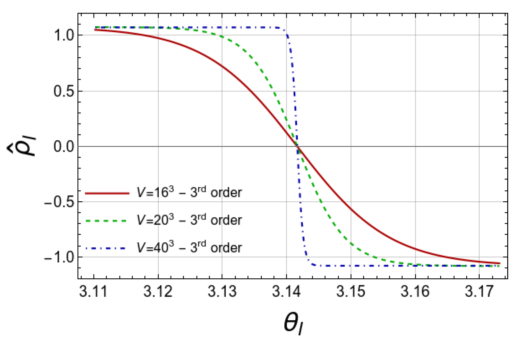
In the Figure 6, we show the approximated ${\widehat{\rho }}_I$ in the vicinity of ${\theta }_I=\pi$ to emphasize its strong dependence on the volume V.

3. Evaluation of Lee–Yang Zeros

The grand partition function $Z_{GC}(\theta ,T,V)$ in the finite volume V can be represented as a polynomial of the baryon fugacity ${\xi }_B=e^{{\mu }_B/T}=e^{\theta }$

$$Z_{GC}(\theta ,T,V)=\sum _{n=-N_{tot}}^{N_{tot}}{Z}_C(n,T,V){\xi }_B^n=e^{-N_{tot}\theta }\sum _{n=0}^{2N_{tot}}{Z}_C(n-N_{tot},T,V){\xi }_B^n,$$

(23)

where $N_{tot}=2N_f{N}_s^3{L}_t$ for Wilson fermions. Zeros of Equation (23) are Lee–Yang zeros. The computation of zeros of the high degree polynomial, Equation (23), is in general a very difficult task. In this work, we employ a very efficient package, MPSolve v.3.1.8 (Multiprecision Polynomial Solver) [28,29], which provides the calculation of polynomial roots with arbitrary precision. In our case, it was enough to use $Z_{nA}$ with an accuracy 12,000 digits to correctly find all LYZ.

Before discussing the results obtained for Equation (5), we would like to describe the observations made for Equation (3). We compare the results obtained for different volumes for the same values of ${\varrho }_{max}=N_{max}/\left(V{T}^3\right)$. We start with ${\varrho }_{max}\approx 0.39$ (corresponding to $N_{max}=25$ for $N_s=16$) and increase it to ${\varrho }_{max}\approx 5.47$. The latter density value corresponds to the maximal value that we can obtain at $T/T_c=1.20$ with $a_5\ne 0$ since respective $Z_{nA}$ become negative for a high enough density, which is related to the fact that ${\widehat{\rho }}_R$ becomes negative for high density in the case of Equation (3). Examining LYZ distribution in detail, we observed a distribution of LYZ similar to that we reported in [25] for $T/T_c=1.35$. It should be noted that the first LYZ on the negative real axes appears at $T/T_c=1.20$ at ${\varrho }_{max}\approx 1.47$ in comparison with ${\varrho }_{max}\approx 1.60$ for $T/T_c=1.35$. It is also worth to note that for fixed $N_s$, all LYZ located on the real negative axis for given value of $N_{max}$ will keep the same position when $N_{max}$ is increased, with new real LYZ appearing closer to ${\xi }_B=0$. This behavior of LYZ is observed for both temperatures $T/T_c=1.35$ and $T/T_c=1.20$.

The approximation with Equation (5) gives us the opportunity to study the behavior of the system in the limit of large values of $N_{max}$ since the density ${\widehat{\rho }}_R$ is positive for all values of ${\theta }_R$.

In Figure 7, the results for LYZ are presented in the complex fugacity plane for two volumes with $N_s=16,40$ and several values of $N_{max}$ for each volume. The general features of the LYZ distribution are very similar to those observed before in Ref. [25] for temperature $T/T_c=1.35$. In the bottom insertion of this figure, ${\xi }_{cl}$ show real LYZ nearest to ${\xi }_B=-1$. One can see that the positions of these LYZ do not depend on ${\rho }_{max}$ but depend on $N_s$. The main difference from the results obtained for $T/T_c=1.35$ is the appearance of additional LYZ branches for ${\varrho }_{max}\approx 8$ for $N_s=40$ and a bit later for smaller volumes; they can be seen in the right insertion of Figure 7. The reason for the branches is not yet completely clear. We can see few such reasons: the insufficient numerical precision in the computation of LYZ, the approximation made in Equation (20) for $Z_{nA}$, or the approximation for the baryon density in Equation (5).

In Ref. [25], we derived the relation connecting the discontinuity of the baryon number density $\Delta {\widehat{\rho }}_I$ to the density of LYZ on the real negative semiaxis:

$$\Delta {\widehat{\rho }}_I=2\pi N_t^{3}g\left({\theta }_R\right).$$

(24)

where $g\left({\theta }_R\right)$ is the density of the LYZ at ${\theta }_I=\pi$. This relation is correct in the limit of an infinite volume. $g\left({\theta }_R\right)$ is defined as

$$g\left({\theta }_R\right)=\frac{1}{N_s^3}\frac{d{N}_{LYZ}\left({\theta }_R\right)}{d{\theta }_R},$$

(25)

where $N_{LYZ}\left({\theta }_R\right)$ is the number of LYZ at $\theta ={\theta }_R+i\pi$. We approximate $g\left({\theta }_R\right)$ as

$$g\left({\theta }_R\right)=\frac{1}{N_s^3\Delta {\theta }_R},$$

(26)

where $\Delta {\theta }_R$ is the distance between adjacent LYZ on the real negative semiaxis. We found that Equation (24) is nicely satisfied at $T/T_c=1.35$ [25] when only terms up to ${\theta }_I^3$ were used in the approximation of the density ${\widehat{\rho }}_I$. Here, we check it for $T/T_c=1.20$ with ${\widehat{\rho }}_I$ approximated by Equation (5). Using Equation (5) we derive for $\Delta {\widehat{\rho }}_I$

$$\Delta {\widehat{\rho }}_I=2\pi \left(a_1-a_3\left({\pi }^2-3{\theta }_R^2\right)-a_7\left({\pi }^6-7\left(3{\pi }^4{\theta }_R^2-5{\pi }^2{\theta }_R^4+{\theta }_R^6\right)\right)\right).$$

(27)

Our results for the lhs and rhs of Equation (24) are presented in the Figure 8. One can see that the numerical value of the discontinuity $\Delta {\widehat{\rho }}_I$ agrees quite well with the analytical prediction at small and large $|{\theta }_R|$. In the intermediate region, we observe a discrepancy with the analytical prediction in the form of oscillations. The maximum of this discrepancy is observed near $|{\theta }_R|=0.5$. By comparing the results for two volumes, one can conclude that with increasing volume the amplitude of the oscillations is increasing but the range of $|{\theta }_R|$ where they are observed is decreasing. Let us note that we observed similar behavior for the density $g\left({\theta }_R\right)$, though less pronounced, for the case of Equation (3), but in the limit of large volumes such oscillations disappeared. The reason for these oscillations is still to be clarified.

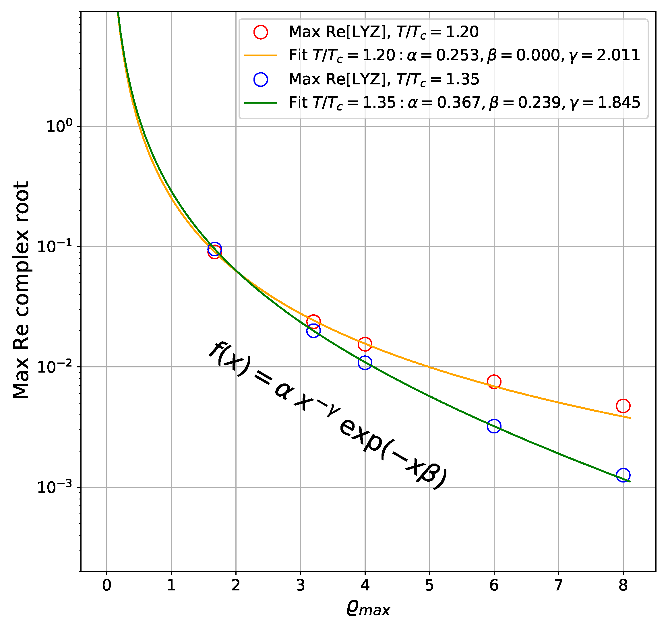
We also studied the behavior of complex LYZ forming small collapsing loop, see Figure 7. In Figure 9, we show the maximal real part of the complex LYZ for $N_s=40$ as a function of ${\varrho }_{max}$ for both $T/T_c=1.2$ and $T/T_c=1.35$. For both temperatures, this value goes to zero, indicating that complex LYZ are collapsing to a point ${\xi }_B=0$, but at $T/T_c=1.2$ this happens slower than for $T/T_c=1.35$. In Figure 9, we also show the fit by the function

$$f\left(x\right)=\frac{\alpha }{x^{\gamma }}{e}^{-\beta x}.$$

(28)

For both temperatures, this fit works quite well. We observed qualitatively similar features of other sides of the loop of complex LYZ, supporting the conclusion that they collapse to a point ${\xi }_B=0$ in the limit of large ${\varrho }_{max}$.

4. Conclusions

We computed the canonical partition functions $Z_{nA}$ and LYZ in $N_f=2$ lattice QCD with Wilson fermion action in the deconfinement phase at $T/T_c=1.20$ above $T_{RW}$ and compared our new results with the results for $T/T_c=1.35$ presented in Ref. [25]. In this paper, we further developed our method to compute the canonical partition functions. The stationary phase method used in computation of $Z_{nA}$ was extended to the third order, see Equation (20).

The method was applied to the case of the imaginary baryon density described by Equation (5), with coefficients $a_i$ determined by fits of the lattice results as shown in Figure 1. We demonstrated that this method to compute $Z_{nA}$ works correctly by reconstructing the input baryon densities. We observed that the relative deviation $\delta {\widehat{\rho }}_I/{\widehat{\rho }}_I$ of the approximated ${\widehat{\rho }}_I$ from the input ${\widehat{\rho }}_I$ becomes substantially better when we improve the approximation for $Z_{nA}$ from the first approximation to the second approximation and then to the third approximation. This agreement improves further when we increase the spatial volume from $V={16}^3$ to $V={40}^3$, as can be seen in the left panel of Figure 5. For the respective relative deviation of ${\widehat{\rho }}_R$ shown in the right panels of same figures, we found that the second and the third approximations provide qualitatively similar precision, which is much better than the precision of the first approximation. In this case, the spatial volume increasing also improves precision quite substantially.

Using the canonical partition functions $Z_{nA}$, we computed LYZ. We found that the general features of LYZ are the same as at $T/T_c=1.35$. Most importantly, there are LYZ on the negative real semi-axes, signaling the first-order Roberge–Weiss transition. In Figure 8, we depict LYZ density $g\left({\theta }_R\right)$ defined in Equation (26) and the discontinuity $\Delta {\widehat{\rho }}_I$ in the average particle-number density at ${\theta }_I=\pi$ and show that the derived relation (24) is satisfied. This figure confirms the reliability of our numerical results for LYZ. In this work, we completed computations at very high densities ${\varrho }_{max}$, reaching values 8.0 (for $N_s=40$) or even 16 (for $N_s=16$), and observed some deviations from regular behavior in the properties of LYZ, indicating the limits of applicability of our method.

We think that the approach to compute the canonical partition functions via the stationary phase method, which we presented in Ref. [25] and developed further in this paper, as well as the results obtained for $Z_{nA}$ and LYZ at high temperatures, will be useful for the computation of these important quantities at lower temperatures where a phase transition or cross-over is present at real values of the chemical potential.